T E C H N I C A L A D V A N C E
Open Access
Comparing lethal dose ratios using probit
regression with arbitrary slopes
Chengfeng Lei and Xiulian Sun
*Abstract
Background:Evaluating the toxicity or effectiveness of two or more toxicants in a specific population often requires specialized statistical software to calculate and compare median lethal doses (LD50s). Tests for equality of LD50s using probit regression with parallel slopes have been implemented in many software packages, while tests for cases of arbitrary slopes are not generally available.
Methods:In this study, we established probit-log(dose) regression models and solved them by the maximum likelihood method using Microsoft Excel. Thez- andχ2-tests were used to assess significance and goodness of fit to the probit regression models, respectively. We calculated the lethal doses (LDs) of the toxicants at different
significance levels and their 95% confidence limits (CLs) based on an accurate estimation of log(LD) variances. We further calculated lethal dose ratios and their 95% CLs for two examples without assuming parallel slopes following the method described by Robertson, et al., 2017.
Results:We selected representative toxicology datasets from the literature as case studies. For datasets without natural responses in the control group, the slopes, intercepts,χ2statistics and LDs calculated using our method were identical to those calculated using Polo-Plus and SPSS software, and the 95% CLs of the lethal dose ratios between toxicants were close to those calculated using Polo-Plus. For datasets that included natural responses in the control group, our results were also close to those calculated using Polo-Plus and SPSS.
Conclusion:This procedure yielded accurate estimates of lethal doses and 95% CLs at different significance levels as well as the lethal dose ratios and 95% CLs between two examples. The procedure could be used to assess differences in the toxicities of two examples without the assumption of parallelism between probit-log(dose) regression lines.
Keywords:Toxicity, Probit regression, Lethal dose ratio, Maximum likelihood
Background
In toxicological, entomological and environmental stud-ies, doses of toxicants that kill a defined proportion of organisms, e.g., the median lethal dose (LD50) which kills 50% of the population, are typically used as indicators of acute toxicity. Comparing the activities of different toxi-cants in a specific population or determining the relative susceptibilities of different populations to a single toxi-cant are common research goals. The relative potency, which assumes that the regression lines of the two toxi-cants being compared are parallel, provides a convenient comparison of the toxicities of two toxicants [1].
However, in practice, many regression lines are not parallel, particularly those derived from bioassays of
tox-icants with different modes of action, or from
same-action toxicants administered to populations with different resistance levels. The 95% confidence limits (CLs) of a lethal dose ratio can be calculated by estimat-ing the slopes and intercepts of two probit regression lines and constructing their variance and covariance matrices. The 95% CLs of this ratio indicate whether the lethal doses of the two toxicants are statistically different from one another [2]. Polo-Plus software, developed by Robertson et al. [3], separately analyzes the data for each substance using probit or logit models based on the joint probability of all observations and calculates lethal dose ratios and their CLs at different significance levels. IBM
* Correspondence:[email protected]
Wuhan Institute of Virology, Chinese Academy of Sciences, Wuhan 430071, Hubei, China
SPSS provides solution to calculate the lethal doses with 95% CLs based on probit or logit models, and also the relative median potency (RMP) assuming that the two regression lines are parallel [4].
In this study, we calculated lethal doses and 95% CLs of toxicants at different significance levels, as well as the lethal dose ratio and its 95% CLs for two toxicants, from probit-log(dose) regression models constructed using the maximum likelihood method in Microsoft Excel. The ef-fectiveness of this method was compared with that of Polo-Plus and IBM SPSS.
Methods
Construction of probit-log(dose) regression models for a single toxicant or population
For a population treated with serial doses (i) of a toxi-cant, in whichnsubjects were treated and rsubjects ex-hibited a characteristic response to each dose, the empirical proportion (p*) of responders was given by
pi ¼ ri
ni: ð
1Þ
wherei= 1 tokand kindicated the number of toxicant doses.
If the characteristic response occurred in the control group (natural response) with proportionC, the propor-tions of responders were corrected using the Abbott equation for each treatment dose [5]:
pi¼
pi−c
1−c : ð2Þ
The corrected proportion (pi) was then converted to a
probit value (yi) [1]:
yi¼Φ−1ð Þpi ; ð3Þ
which was calculated asyi= NORM.S.INV(pi) in Excel. A provisional regression line betweenyiand the
loga-rithm of the dose (xi) was established:
yi¼α0þβ0xi: ð4Þ
In the regression equation, i= 1 tom, where mis the number of toxicant doses at which the corrected propor-tion was not equal to 1 or 0. The intercept (α0) and slope (β0) could be calculated by the least-squares pro-cedure and were retrieved using the INTERCEPT(yi, xi)
and SLOPE(yi,xi) functions, respectively, in Excel.
We then calculated the expected probits (Y) for all dose sets, included those where the corrected proportion was 1 or 0:
Yi¼α0þβ0xi: ð5Þ
In Eq. (5),i= 1 tok.
We next calculated the expected response proportion (Pi) for each dose set [1].
Pi¼Φð Þ Yi ð1−CÞ þC; ð6Þ
where Φ(Yi) returned the cumulative probability of the
standard normal distribution corresponding to (Yi),
ob-tainable using the NORM.S.DIST (Yi) function in Excel,
and C was the natural response proportion, if one existed, in Eq. (2).
The working probit (yi) was calculated from the
fol-lowing eq. [1]:
yi¼Yi−
Pi
Ziþ
pi
Zi; ð
7Þ
where
Zi¼
1 ffiffiffiffiffiffi 2π
p e−0:5Y2i: ð8Þ
An optimized set of expected probits was then derived from the linear regression equation of working probits weighted on xi, with each yi being assigned a weight,
niwi, where wi was the weighting coefficient. This was
calculated as previously described [1]
wi¼
Z2i Piþ
C
1−C
1−Pi
ð Þ
; ð9Þ
whereCwas the natural response proportion in Eq. (2).
The slope β of the working probit-log10(dose) regres-sion equation was
β¼
Pk
i¼1niwiðxi−xÞðyi−yÞ
Pk
i¼1niwiðxi−xÞ2
: ð10Þ
The interceptαof the working probit regression equa-tion was
α¼y−βx; ð11Þ
whereȳwas the average ofyandxwas the average ofx:
y¼
Pk i¼1niwiyi
Pk i¼1niwi
;x¼
Pk i¼1niwixi
Pk i¼1niwi
: ð12Þ
The standard error ofβwas [1]
σ βð Þ ¼
ffiffiffiffiffiffiffiffiffiffiffiffiffiffiffiffiffiffiffiffiffiffiffiffiffiffiffiffiffi 1 Pk
i¼1niðxi−xÞ2
s
; ð13Þ
and the standard error ofαwas [6]
σ αð Þ ¼
ffiffiffiffiffiffiffiffiffiffiffiffiffiffiffiffiffiffiffiffiffiffiffiffiffiffiffiffiffiffiffiffiffiffiffiffiffiffiffiffi 1
Pk i¼1niwi
þx2σ βð Þ2
s
: ð14Þ
X2¼Xk
i¼1
niðpi−PiÞ2
Pið1−PiÞ : ð
15Þ
The significance level p of the χ2 statistic was calcu-lated as the right-tailed probability of the chi-squared
distribution (CHISQ.DIST.RT) with k – 2 degrees of
freedom (d.f.).
A significantχ2statistic (p< 0.05) might indicate either that the population did not respond independently or that the fitted probit-log(dose) regression line did not adequately describe the dose-response relationship in the test samples.
To get an optimal fit of the probit-log10(dose) regres-sion, we substituted αand βfor α0and β0and repeated the calculations of Eq. (5) to Eq. (15) until a stableχ2 ap-peared, indicating convergence. This procedure was a maximum likelihood (ML) method [1].
The significance of the slope was assessed using the z test [7],
Z¼ β
σ βð Þ ð16Þ
If the absolute z-value was less than 1.96, the regres-sion slope was not significant and the data were ex-cluded from further analysis. Similarly, we might test the significance of the intercept (α).
The heterogeneity factor h of the regression equation was calculated to adjust for largeχ2.hwas defined as [1]
h¼ χ
2
k−2: ð17Þ
If h< 1, the model provided a good fit to the data. Otherwise, standardized residuals were plotted to iden-tify outliers or other possible causes of poorness of fit [8]. Each residual defined the difference between the ob-served ri and the expected response number (niPi) for
each dose. The residuals were standardized by dividing them by their standard errors, ffiffiffiffiffiffiffiffiffiffiffiffiffiffiffiffiffiffiffiffiffiniPið1−PiÞ
p
. For models providing a good fit, the standardized residuals fell mostly between−2 and 2 [8]. Standardized residuals dis-tributed randomly showed no systematic patterns or ten-dencies toward positive or negative sign.
Calculation of the lethal doses of toxicants or populations and their 95% CLs
In this step, we first calculated the logarithms of the doses (θπ) at which levels of interest (π) gave the ex-pected response proportion:
θπ¼yπβ−α ð18Þ
whereyπwas theπthpercentile of the probit distribution
curve calculated in Excel using NORM.S.INV(π) for the
probit distribution. For example, ifπ= 10, 50, 90 and 99,
yπwas calculated as−1.282, 0, 1.282 and 2.326. Theπthlethal dose was then calculated as
LDπ¼10θπ: ð19Þ
The standard error ofθπ,σ(θπ), was given by [1]
σ θð Þ ¼π 1β
ffiffiffiffiffiffiffiffiffiffiffiffiffiffiffiffiffiffiffiffiffiffiffiffiffiffiffiffiffiffiffiffiffiffiffiffiffiffiffiffiffiffiffiffiffiffiffiffiffiffiffiffiffiffiffiffiffiffi 1
Pk i¼1niwi
þ ðθπ−xÞ
2 Pk
i¼1niwiðxi−xÞ2
s
: ð20Þ
The 95% CL of the LDπwas then given as
10θπt0:05;k−2σ θð Þπ : ð21Þ t0.05, k−2 returned the two-tailed inverse of the Student’s t-distribution at α= 0.05 with d.f. = k - 2 [T.INV.2 T(0.05,k-2)].
The g value could be calculated to adjust if the confi-dence limits were valid. Thegvalue was given as [9]:
g¼t 2σ βð Þ2
β2 h
: ð22Þ
If p(χ2) was less than 0.15, t= 1.96 and h*= 1; other-wise,h*=handt=t0.05,k−2[4]. Ifgexceeded 1, the CLs for the LDπdid not have practical importance [1].
The above steps were repeated to determine all param-eters for the second toxicant for the same population, or the same toxicant in the second population.
Comparison of lethal dose ratios of two toxicants or populations
If there were l toxicants or populations in the experi-ment, then we compared the LDπvalues of the first (as a reference) to those of others. We first calculated the dif-ference between the log(doses) yielding the expected re-sponse proportions (πth percentile) for toxicants or populations 1 andj(j =2 tol),θπ1j=θπ1-θπj. Its
stand-ard error was given by [2]
σ θπ1j
¼ ffiffiffiffiffiffiffiffiffiffiffiffiffiffiffiffiffiffiffiffiffiffiffiffiffiffiffiffiffiffiffiffiffiffiffiffiσ θð π1Þ2þσ θπj 2 q
: ð23Þ
The ratio of the two lethal doses was then given as
Ratioð Þ ¼1j 10θπ1−θπj; ð24Þ
and the 95% CLs were
10θπ1j1:96σ θð Þπ1j : ð25Þ
Test for parallelism of the two regression equations Although the above procedures did not assume equal slopes of the two regression lines, the specific LDπ level used depended on the parallelism of the regression lines. To examine parallelism of the two regression lines, we used thez-test [10]:
z¼ β1−βj
ffiffiffiffiffiffiffiffiffiffiffiffiffiffiffiffiffiffiffiffiffiffiffiffiffiffiffiffiffiffiffiffiffi σ βð Þ1
2þσ β
j
2
r : ð26Þ
If the absolute z-value exceeded 1.96, the two regres-sions were non-parallel; otherwise, they were parallel.
Case studies
The above procedures might be executed on an Excel (version 2010 or higher) spreadsheet (provided as an Additional file 1). To compare the results of the ML procedure in Excel with those of Polo-Plus and SPSS, we extracted bioassay data from the literature: (1) chrysan-themum aphids dosed with Rotenone, Deguelin, and a mixture of these two substances [11], (2) three popula-tions, Fairfax, Pixley and Schaefer, of the pest bug “Wicked Witch of the West” dosed with deltamethrin [12], and (3) two populations, BugRes and BugLab, of Godfather larvae dosed with pyrethroid [2] (Table1).
Results
Slopes, intercepts and significance testing of probit-log(dose) models fitted to the example data
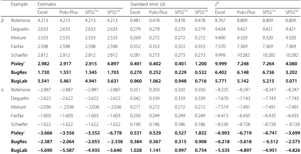
When we implemented the ML procedure to solve the probit-log(dose) equations for the three sample data in Excel, for the datasets in which there was no natural response (e.g., Rotenone, Deguelin, Mixture, Fairfax and Schaefer), the slope (β) and intercept (α) estimates of the converged probit-log(dose)
regres-sion were identical to those calculated using
Polo-Plus and SPSS (with two methods, SPSS1 and
SPSS2, to include the natural response proportion,C,
by inputting the value of C and calculating it from
the data, respectively) (Table 2). The standard errors of both β and α, calculated by Eq. (13) and Eq. (14), were close but not identical to those calculated using Polo-Plus and SPSS (Table 2). When the data sets in-cluded natural responses (e.g., Pixley, BugRes and BugLab), β and α, as well as their standard errors, were close to those produced by Polo-plus and SPSS. The results of our method and Polo-Plus were closer
to those calculated using SPSS1 method than those
calculated using SPSS2method (Table 2, Bold items). The probit-log(dose) regression model assumes a linear relationship between the logarithm of serial doses and the probit of the response proportions. When z-tests (this study and SPSS) or the t-ratios (Polo-Plus) were used to evaluate the significance of
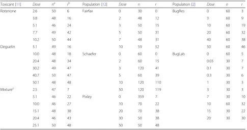
Table 1Selected bioassay data for toxicants in experimental populations
Toxicant [11] Dose na rb Population [12] Dose n r Population [2] Dose n r
Rotenone 2.6 50 6 Fairfax 0 30 0 BugRes 0 60 3
3.8 48 16 2 48 12 3 60 9
5.1 46 24 3 50 15 10 60 19
7.7 49 42 5 50 31 20 60 32
10.2 50 44 7 48 31 40 60 38
Deguelin 5.1 49 16 10 59 52 50 60 46
10.0 48 18 Schaefer 0 60 0 BugLab 0 60 5
20.4 48 34 2 60 15 0.03 30 7
30.2 49 47 3 120 41 0.1 30 7
40.7 50 47 5 60 39 0.3 30 6
50.1 48 48 10 120 110 1 30 3
Mixturec 2.5 47 7 50 120 119 3 30 3
5.1 46 22 Pixley 0 359 7 7 30 10
10.0 46 27 10 70 22 10 60 32
15.1 48 38 20 70 38 15 30 22
20.4 46 43 30 50 38 20 30 30
25.1 50 48 50 50 48
a
nwas the total number of subjects administrated at each dose
b
rwas the number of subjects exhibited a characteristic response to each dose
c
the regressions, all z values and t-ratios for both β
and α estimates calculated using all four methods
exceeded 1.96 (Table 2), indicating that all regression
parameters were significant. If the z-value for the
slope was less than 1.96, the regression model would be insignificant and the dataset should be excluded from further analysis.
Goodness-of-fits of the probit-log(dose) regressions While z-tests evaluated whether a linear relationship existed between the probits and the log(dose), χ2 tests are usually used to test the goodness-of-fit of the log(dose)-probit regression model. For datasets that did not include natural responses, the χ2 and h values calculated in this study were identical to those
calcu-lated using Polo-Plus and SPSS (Table 3). When the
datasets included natural responses, the χ2 and h
values were close to those produced by Polo-plus and SPSS. Again, the results of our method and Polo-Plus
were closer to those calculated using SPSS1 method
than those calculated using SPSS2 method (Table 3,
Bold items).
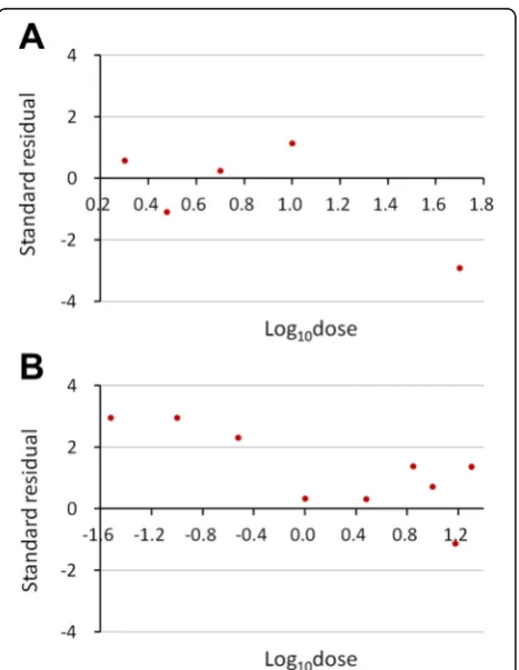
For some datasets, χ2 was not significant but h was greater than 1 (Table 3). When standardized residuals were plotted against log(doses), one or more outliers
were observed (outside the bounds of −2 to 2) in the Schaefer and BugLab data. For the BugLab data espe-cially, the standardized residuals were not distributed randomly and showed a tendency toward positive sign (Fig. 1), indicating that this data should be fitted using other models [13].
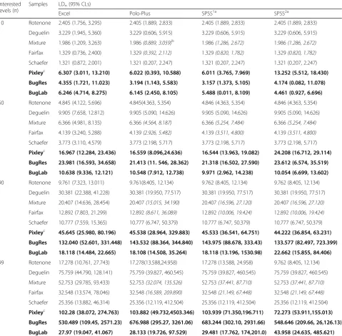
LD10, LD50, LD90and LD99estimates with 95% CLs
We further compared the LDπs and their 95% CLs
calculated using these four methods. For datasets that did not include natural responses, the LDπs calculated in this study were identical to those calculated using Polo-Plus and SPSS, and the 95% CLs of LDπs calcu-lated using our method were close but not identical
to those produced by Polo-Plus and SPSS (Table 4).
For datasets that included natural responses, the LDπs and their 95% CLs were close but not identical to those calculated using Polo-plus and SPSS. The re-sults of our method and Polo-plus were closer to those calculated using SPSS1 method than those cal-culated using SPSS2method (Table 4, Bold items).
Comparison of lethal dose ratios between two samples For datasets that did not include natural responses,
the LDπ ratios calculated using our method were
Table 2Slopes, intercepts and results of significance testing for the example data fitted to the probit-log(dose) regression models
using the ML procedure (Excel), Polo-Plus and SPSS
Example Estimates Standard error (σ) zb
Excel Polo-Plus SPSS1a SPSS2a Excel Polo-Plus SPSS1a SPSS2a Excel Polo-Plus SPSS1a SPSS2a
β Rotenone 4.213 4.213 4.213 4.213 0.481 0.478 0.478 0.478 8.767 8.809 8.809 8.809
Deguelin 2.633 2.633 2.633 2.633 0.279 0.279 0.279 0.279 9.434 9.421 9.421 9.421
Mixture 2.533 2.533 2.533 2.533 0.269 0.272 0.272 0.272 9.400 9.320 9.320 9.320
Fairfax 2.598 2.598 2.598 2.598 0.352 0.353 0.353 0.353 7.370 7.369 7.369 7.369
Schaefer 2.812 2.812 2.812 2.812 0.281 0.273 0.273 0.273 9.999 10.282 10.282 10.282
Pixleyc 2.982 2.917 2.915 4.897 0.401 0.402 0.401 1.200 9.999 7.248 7.264 4.080
BugRes 1.730 1.551 1.545 1.703 0.270 0.252 0.229 0.532 6.402 6.148 6.736 3.202
BugLab 5.541 5.461 4.941 3.631 0.960 1.062 0.948 0.716 5.771 5.142 5.215 5.071
α Rotenone −2.887 −2.887 −2.887 −2.887 0.351 0.350 0.350 0.350 −8.225 −8.247 −8.247 −8.247
Deguelin −2.622 −2.622 −2.622 −2.622 0.342 0.339 0.339 0.339 −7.670 −7.743 −7.743 −7.743
Mixture −2.036 −2.036 −2.036 −2.036 0.271 0.272 0.272 0.272 −7.519 −7.491 −7.491 −7.491
Fairfax −1.603 −1.603 −1.603 −1.603 0.250 0.249 0.249 0.249 −6.413 −6.435 −6.435 −6.435
Schaefer −1.622 −1.622 −1.622 −1.622 0.190 0.186 0.186 0.186 −8.530 −8.728 −8.728 −8.728
Pixleyc −3.666 −3.556 −3.552 −6.778 0.531 0.529 0.527 1.832 −6.903 −6.719 −6.741 −3.699
BugRes −2.387 −2.064 −2.053 −2.338 0.384 0.367 0.315 0.908 −6.218 −5.618 −6.512 −2.575
BugLab −5.690 −5.587 −4.935 −3.640 1.028 1.141 0.997 0.754 −5.535 −4.897 −4.951 −4.826
a
SPSS includes the natural responses proportion (C) by two methods: 1, inputting the value ofC; and 2, calculating the correctedpfrom the data. Thed.f.=k−2 in method 1, while it wask-3 in method 2
b
Polo-Plus used thet-ratio to test the significance of the linear regression. The significance criterion for thet-ratio (α= 0.05) was 1.96 (t-distribution withd.f.=∞). This significance level was identical to that of theztest
c
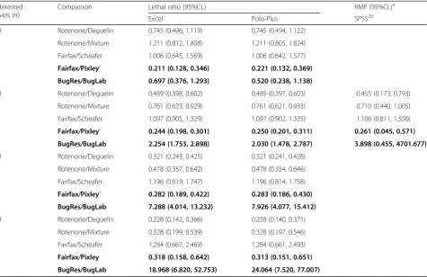
identical to those calculated using Polo-Plus and their 95% CLs were also close. For datasets that included natural responses, LDπ ratios and their 95% CLs cal-culated using our method were similar to those calcu-lated using Polo-Plus (Table 5, Bold items). The LD50 ratios and their 95% CLs calculated using our method
were closer to those calculated using Polo-Plus than to the relative median potency (RMP) calculated using SPSS (Table 5).
When judged by whether the 95% CLs of lethal ratios included 1.0, all methods reached the same conclusions for toxicity differences between two samples (Table5).
Comparisons of two regression slopes
Parallelism between paired regression equations was ex-amined usingz-tests. The conclusions of our method for the five regression pairs were identical to those arrived at by Polo-Plus and SPSS, which usedχ2tests (Table6).
Discussion
Many methods have been developed to calculate the lethal or effective doses of toxicants and their confidence limits. Probit analysis, developed by Bliss [14] and improved by Finney [11], is one such commonly-used method. To cal-culate the parameters of the probit-log(dose) regression, Finney suggested fitting the regression line by eye as pre-cisely as possible and obtaining parameters, such as slopes and intercepts, of the provisional regression line at the first stage. Thereafter, one calculates the working probits Y, and repeats this process with the new set of Yvalues; when the iterations converge, this gives a precise estimate of the linear regression parameters [1]. In this study, we calculated slopes and intercepts for the provisional regres-sion line by the least-squares procedure, and calculated working probits and performed the iteration procedure (ML) using the popular software program, Microsoft Excel. We obtained similar results to those obtained using Polo-Plus and SPSS.
Several software packages, such as Polo-Plus and SPSS, might be used to calculate the lethal doses and 95% CLs at different significance levels, and even test the equality of the lethal doses. Such professional
Fig. 1Standardized residuals versus log(doses) after fitting the Schaefer (a) and Buglab (b) dataset to probit-log(dose) models
Table 3Goodness-of-fit of the probit-log(dose) regression models calculated from the example data using the ML procedure
(Excel), Polo-Plus and SPSS
Examples χ2 hb gc
Excel Polo-Plus SPSS1a SPSS2a Excel Polo-Plus SPSS1a SPSS2a Excel
Rotenone 1.729 1.729 1.729 1.729 0.576 0.576 0.576 0.576 0.050
Deguelin 12.026d 12.026d 12.026d 12.026d 3.006 3.006 3.006 3.006 0.260
Mixture 4.995 4.995 4.995 4.995 1.249 1.249 1.249 1.249 0.043
Fairfax 3.754 3.754 3.754 3.754 1.251 1.251 1.251 1.251 0.071
Schaefer 11.384d 11.384d 11.384d 11.384d 3.795 3.795 3.795 3.795 0.384
Pixleye 2.671 2.708 2.712 0.064 1.335 1.354 1.356 0.032 0.069
BugRes 1.382 1.358 1.362 1.266 0.461 0.453 0.454 0.633 0.094
BugLab 13.555 11.081 27.454 10.181 1.936 1.583 3.922 1.697 0.325
a
SPSS includes the natural responses proportion by inputting the value ofC, and SPSS calculates the correctedpfrom the data
b
h, heterogeneity factor (see Eq.(17)). SPSS did not giveh. To compare the results from this study and Polo-Plus, it was shown ash=χ2
/d.f. here
c
The g value was calculated as Eq.(22). Polo-Plus and SPSS did not calculate thegvalues
dχ2
indicated the goodness-of-fit test was significant atα= 0.05
e
statistical programs are difficult to handle for common toxicologists and environmental ecologists, and are easily abused. Excel in the Microsoft Office Package is the most popular statistical program around the globe. As to the Excel spreadsheet developed in this study, the users are easily to trace the procedure which is used to solve the re-gression equations, and calculate the CLs of a lethal dose and also the lethal dose ratios. They may further redevelop it easily according to their request.
χ2
values were used as indicators of the goodness-of-fit of the probit-log(dose) regressions as the iteration pro-ceeded. The equations
χ2¼Xnw y−yð Þ2− P
nw x−xð Þðy−yÞ
ð Þ2
P
nw x−xð Þ ð27Þ
or
Table 4LD10, LD50, LD90and LD99values with their 95% CLs for the example data fitted to probit-log(dose) regression models
using the ML procedure (Excel), Polo-Plus and SPSS Interested
levels (π)
Samples LDπ(95% CLs)
Excel Polo-Plus SPSS1a SPSS2a
10 Rotenone 2.405 (1.756, 3.295) 2.405 (1.889, 2.833) 2.405 (1.889, 2.833) 2.405 (1.889, 2.833)
Deguelin 3.229 (1.945, 5.360) 3.229 (0.606, 5.915) 3.229 (0.606, 5.915) 3.229 (0.606, 5.915)
Mixture 1.986 (1.209, 3.263) 1.986(0.889, 3.059)b 1.986(1.286, 2.672) 1.986(1.286, 2.672)
Fairfax 1.329 (0.736, 2.400) 1.329(0.392, 2.112) 1.329(0.820, 1.782) 1.329(0.820, 1.782)
Schaefer 1.321 (0.872, 2.001) 1.321 (0.207, 2.247) 1.321 (0.207, 2.247) 1.321 (0.207, 2.247)
Pixleyc 6.307 (3.011, 13.210) 6.022 (0.393, 10.588) 6.011 (3.765, 7.969) 13.252 (5.512, 18.430)
BugRes 4.355 (1.721, 11.023) 3.194 (1.143, 5.583) 3.157 (1.373, 5.105) 4.174 (0.082, 11.078)
BugLab 6.246 (4.714, 8.275) 6.145 (2.450, 8.105) 5.488 (0.011, 8.109) 4.461 (0.927, 6.696)
50 Rotenone 4.845 (4.122, 5.696) 4.845(4.363, 5.354) 4.846 (4.363, 5.354) 4.846 (4.363, 5.354)
Deguelin 9.905 (7.658, 12.812) 9.905 (5.090, 14.626) 9.905 (5.090, 14.626) 9.905 (5.090, 14.626)
Mixture 6.366 (4.981, 8.135) 6.366(4.564, 8.187) 6.366(5.254, 7.484) 6.366(5.254, 7.484)
Fairfax 4.139 (3.240, 5.288) 4.139(2.926, 5.482) 4.139(3.511, 4.800) 4.139(3.511, 4.800)
Schaefer 3.773 (3.110, 4.579) 3.773 (2.198, 5.717) 3.773 (2.198, 5.717) 3.773 (2.198, 5.717)
Pixleyc 16.967 (12.284, 23.436) 16.559 (8.096,24.636) 16.544 (13.963, 19.082) 24.208 (16.712, 29.114)
BugRes 23.981 (16.593, 34.658) 21.413 (11. 546, 28.362) 21.318 (16.502, 27.590) 23.612 (6.574, 35.519)
BugLab 10.638 (9.336, 12.121) 10.548 (7.912, 12.738) 9.971 (2.962, 14.238) 10.054 (6.699, 13.602)
90 Rotenone 9.761 (7.323, 13.011) 9.761(8.405, 12.134) 9.762 (8.405, 12.134) 9.762 (8.405, 12.134)
Deguelin 30.381 (22.388, 41.228) 30.381 (19.950, 77.517) 30.381 (19.950, 77.517) 30.381 (19.950, 77.517)
Mixture 20.407 (14.636, 28.454) 20.407(15.015, 34.190) 20.407(16.596, 27.120) 20.407(16.596, 27.120)
Fairfax 12.892 (7.803, 21.299) 12.892(8.611, 36.089) 12.892(10.006, 19.424) 12.892(10.006, 19.424)
Schaefer 10.777 (7.559, 15.365) 10.777 (6.747, 50.379) 10.777 (6.747, 50.379) 10.777 (6.747, 50.379)
Pixleyc 45.645 (25.980, 80.196) 45.538 (28.964, 329.883) 45.533 (36.541, 64.751) 44.222 (36.854, 63.231)
BugRes 132.040 (52.601, 331.448) 143.532 (88.364, 344.840) 143.975 (88.678, 333.43) 133.577 (82.497, 723.399)
BugLab 18.118 (14.484, 22.665) 18.108 (14.508, 35.264) 18.118 (13.196, 1530.98) 22.662 (15.855, 84.406)
99 Rotenone 17.278 (10.761, 27.743) 17.278(13.588,24.958) 17.278 (13.588, 24.958) 9.762 (8.405, 12.134)
Deguelin 75.759 (44.790, 128.141) 75.759 (39.827, 460.545) 75.759 (39.827, 460.545) 75.759 (39.827, 460.545)
Mixture 52.753 (29.785, 93.433) 52.753(32.074, 135.526) 52.753(37.441, 87.710) 52.753(37.441, 87.710)
Fairfax 32.548 (13.574, 78.046) 32.548(16.589, 209.890) 32.548(21.149, 67.448) 32.548(21.149, 67.448)
Schaefer 25.356 (13.882, 46.314) 25.356 (12.119, 412.504) 25.356 (12.119, 412.504) 25.356 (12.119, 412.504)
Pixleyc 102.28 (38.072, 274.763) 103.882 (49.732,4503.346) 103.939 (71.350,196.711) 72.273 (53.911,155.013)
BugRes 530.489 (109.45, 2571.23) 676.988 (295.27, 3261.06) 683.244 (302.10, 2931.66) 548.646 (209.66, 26,126.13)
BugLab 27.97 (19.047, 41.067) 28.133 (19.726, 97.529) 29.481 (17.762, 174,201.0) 43.958 (24.635, 485.621)
a
SPSS includes the natural responses proportion by inputting the value ofC, and SPSS calculates the correctedpfrom the data
b
Data in italic brackets indicated that he 95% CLs of LDπcalculated using Polo-Plus were not identical to those calculated using SPSS
c
χ2¼Xðr−nPÞ 2
nPð1−PÞ ð28Þ
could also be applied [1]. When there were no nat-ural responses in the datasets, these two equations, along with Eq. (15), gave the same results when the iterations converged, and these results were identical to those produced by Polo-Plus and SPSS. When the datasets included natural responses, Eq. (27) always gave the smallest χ2 value, Eq. (28) always gave the largest value, while Eq. (15) gave an intermediate value which was closer to the output of Polo-Plus
and SPSS (data not shown). During iteration for some datasets, the χ2 values produced from all these three equations might increase [1]. Most regression models converged after several iterations, and we reported the results after 20 iterations, as this was the default maximum used by SPSS.
Strictly speaking, the 95% CLs of LDπ were the values
of x for which the boundaries of the fiducial band
attained the relevant value of yπ. The exact CLs of θπ
could be calculated by constructing the variance matri-ces of the slope (var(β)) and intercept (var(α)) and their covariance (cov(α,β)) matrices as follow [1,9]:
Table 5Lethal dose ratios for the examples fitted to the probit-log(dose) regression models calculated by the ML procedure (Excel),
Polo-Plus and SPSS Interested
levels (π)
Comparison Lethal ratio (95%CL) RMP (95%CL)a
Excel Polo-Plus SPSS2b
10 Rotenone/Deguelin 0.745 (0.496, 1.119) 0.745 (0.494, 1.122)
Rotenone/Mixture 1.211 (0.812, 1.808) 1.211 (0.805, 1.824)
Fairfax/Scheafer 1.006 (0.645, 1.569) 1.006 (0.642, 1.577)
Fairfax/Pixleyc 0.211 (0.128, 0.346) 0.221 (0.132, 0.369)
BugRes/BugLab 0.697 (0.376, 1.293) 0.520 (0.238, 1.138)
50 Rotenone/Deguelin 0.489 (0.398, 0.602) 0.489 (0.397, 0.603) 0.455 (0.173, 0.793)
Rotenone/Mixture 0.761 (0.623, 0.929) 0.761 (0.621, 0.933) 0.710 (0.440, 1.005)
Fairfax/Scheafer 1.097 (0.905, 1.329) 1.097 (0.902, 1.335) 1.106 (0.811, 1.550)
Fairfax/Pixleyc 0.244 (0.198, 0.301) 0.250 (0.201, 0.311) 0.261 (0.045, 0.571)
BugRes/BugLab 2.254 (1.753, 2.898) 2.030 (1.478, 2.787) 3.898 (0.455, 4701.677)
90 Rotenone/Deguelin 0.321 (0.243, 0.425) 0.321 (0.241, 0.428)
Rotenone/Mixture 0.478 (0.357, 0.642) 0.478 (0.354, 0.646)
Fairfax/Scheafer 1.196 (0.819, 1.747) 1.196 (0.814, 1.758)
Fairfax/Pixleyc 0.282 (0.189, 0.422) 0.283 (0.186, 0.430)
BugRes/BugLab 7.288 (4.014, 13.232) 7.926 (4.077, 15.412)
99 Rotenone/Deguelin 0.228 (0.142, 0.366) 0.228 (0.140, 0.371)
Rotenone/Mixture 0.328 (0.199, 0.539) 0.328 (0.197, 0.546)
Fairfax/Scheafer 1.284 (0.667, 2.469) 1.284 (0.661, 2.493)
Fairfax/Pixley 0.318 (0.158, 0.642) 0.313 (0.151, 0.651)
BugRes/BugLab 18.968 (6.820, 52.753) 24.064 (7.520, 77.007)
a
RMP, relative median potency. We did not show the RMP of SPSS by inputtingCmethods because of differentCvalues in the two samples
b
SPSS calculates the correctedpfrom the data. We did not calculate RMP with SPSS by inputtingCmethods because of differentCvalues in the two samples
c
Bold items indicated the data sets included natural responses in the control group
Table 6Tests of parallelism between the probit-log(dose) regression lines calculated using the ML procedure (Excel), Polo-Plus and SPSS
Comparison Excel Polo-Plus SPSS2a
z Parallelism χ2
(d.f.= 1) Parallelism χ2(d.f.= 1) Parallelism
Rotenone vs Deguelin 2.844 Rejected 8.41 Rejected 10.216 Rejected
Rotenone vs Mixture 3.049 Rejected 9.68 Rejected 9.284 Rejected
Fairfax vs Scheafer 0.475 Accepted 0.23 Accepted 0.000 Accepted
Fairfax vs Pixley 0.720 Accepted 0.36 Accepted 0.598 Accepted
BugRes vs BugLab 3.821 Rejected 22.10 Rejected 24.840 Rejected
a
θπþ g
1−g θπ− covðα;βÞ
varð Þβ
β t 1−g
ð Þ
ffiffiffiffiffiffiffiffiffiffiffiffiffiffiffiffiffiffiffiffiffiffiffiffiffiffiffiffiffiffiffiffiffiffiffiffiffiffiffiffiffiffiffiffiffiffiffiffiffiffiffiffiffiffiffiffiffiffiffiffiffiffiffiffiffiffiffiffiffiffiffiffiffiffiffiffiffiffiffiffiffiffiffiffiffiffiffiffiffiffiffiffiffiffiffiffiffiffiffiffiffiffiffiffiffiffiffiffiffiffiffiffiffiffiffiffiffiffiffiffiffiffiffi
varð Þα−2θπcovðα;βÞ þθπ2varð Þβ−g varð Þα−covðα;βÞ 2
varð Þβ
! v
u u
t :
ð29Þ
It has been theorized that, in practice, the method for de-termining 95% CLs of LDπ most often performed suffi-ciently good based on a trustworthy value for the variance ofθπas Eq. (20) [1,15]. It was suggested that 95% CLs of LDπ could be calculated using the formula 10θπ1:96σðθπÞ [15]. The results of this equation were close to those calcu-lated using Eq. (29) when the dose number (k) was large (e.g., close to 10), while the CLs were much narrow than those calculated exactly using Eq. (29) whenkwas small. By contrast, the results given by Eq. (21) were nearer to those calculated exactly at different levels of k. The 95% CLs of LDπcalculated using Polo-Plus were often identical to those calculated using SPSS when there was no natural response, with some exceptions (e.g., the Mixture and Fairfax data; Table4, italic brackets, although thegvalues were not large for both of these cases).
While it is common to find estimates of LDs obtained from probit analyses in the toxicology literature, it is less common to find a hypothesis test procedure to determine whether estimated differences between LDs are statistically significant [16]. Relative potency has been frequently used [1, 4], but this method assumes the regression lines being com-pared are parallel. When the regression lines were parallel, the LDs and their 95% CLs for two toxicants calculated from the two datasets simultaneously were similar to those calcu-lated from the datasets separately. However, when the re-gression lines were not parallel, the LDs and their 95% CLs calculated from the two datasets simultaneously were quite different from those calculated from the datasets separately.
In cases where the data are suggestive of a trend to-ward significant differences between LD50s, the use of
non-overlapping CLs for LD50 values has frequently
been proposed as a criterion for assessing significance, while use of this criterion is thought to be conservative [17, 18]. An alternative method involves calculating the variances ofθπusing the delta-method:
varð Þ ¼θπ 1
β2 varð Þ þα 2θπcovðα;βÞ þθπ 2
varð Þβ
; ð30Þ
calculating the ratio of the LDs as in Eq. (24), then cal-culating the 95% CLs of the ratio as in Eq. (25) [2]. If the 95% CLs of the ratio include 1.0, the LDs of the two samples are not significantly different. We followed this procedure in this study, but we calculated the standard error ofθπas in Eq.(20) by the maximum likelihood
pro-cedure. We obtained 95% CLs of the LD ratio similar to those obtained using Polo-Plus.
Biologically, the slope of a probit or logit regression line represents the change in the proportion of responders per unit change in dose. Toxicological evidence suggested that the slope of a dose–response regression line reflected host enzyme activity [19]. Thus, non-parallel lines might indicate different modes of action of the two toxicants. Par-allelism between regression pairs was essential for deter-mining the level at which to compare the effects of two toxicants. Generally, there were three main categories of parallelism: (i) the two regression lines were statistically parallel (e.g., Fairfax vs Pixley; Fig.2a); (ii) the two regres-sion lines were not statistically parallel but did not cross
within the dominant region (20–80%) of the response pro-portions (e.g., Rotenone vs Deguelin; Fig.2b); and (iii) the two regression lines crossed around the median lethal dose (e.g., BugRes vs BugLab; Fig.2c). In the first case, reporting the LD50s of the two toxicants and their ratios was suffi-cient. In the second case, one should report both LD50s and LD90s (and/or LD10s) and their ratios. In the third case, reporting the ratios of LD10s, LD50s, LD90s is mean-ingless, but the significance of difference between the two slopes should be valid.
Conclusions
We successfully developed a method to calculate the le-thal doses of a toxicant at different significance levels, and compare lethal dose ratios using probit-log(dose) re-gression by the ML procedure implemented in Microsoft Excel. Lethal doses calculated using this method at dif-ferent significance levels, as well as lethal dose ratios with their 95% CLs, were identical or close to those cal-culated using Polo-Plus and SPSS. When judged by whether the 95% CLs of the lethal ratios included 1.0, all methods reached the same conclusions regarding tox-icity differences between two samples.
Additional file
Additional file 1:Calculation of LDs and their ratios.xlsx (344 kb), which requires Microsoft Excel 2010 or higher. It is available via a link:https:// figshare.com/s/f94393f752fcc15faea7. (XLSX 1493 kb)
Abbreviations
95% CLs:95% confidence limits; LD50: Median lethal dose; ML: Maximum
likelihood; RMP: Relative median potency
Funding
We appreciate the support of the National Key Research and Development Program of China (2017YFD0201206), and the WIV“One-Three-Five”strategic programs (Y602111SA1).
Availability of data and materials
Additional file1is available via a link:https://figshare.com/s/f94393f752fcc15faea7.
Authors’contributions
XS and CL conceived and designed the study. CL edited the Excel file, analyzed the data and prepared the manuscript. XS revised the manuscript. Both authors read and approved the final manuscript.
Ethics approval and consent to participate Not applicable.
Consent for publication Not applicable.
Competing interests
The authors declare that they have no competing interests.
Publisher’s Note
Springer Nature remains neutral with regard to jurisdictional claims in published maps and institutional affiliations.
Received: 3 August 2018 Accepted: 24 September 2018
References
1. Finney DJ. Probit Analysis. 3rd ed. Cambridge: Cambridge University Press; 1971. 2. Robertson JL, Jones MM, Olguin E, Alberts B. Bioassays with arthropods. 3rd
ed. Boca Raton, FL: CRC Press, Taylor & Francis Group; 2017. 3. LeOra Software. Polo-Plus, POLO for windows. Petaluma, CA: LeOra
Software, 107 B St, 94952; 2007.
4. SPSS Inc., IBM Corp. IBM SPSS statistics 20.0. Chicago, IL: SPSS Inc.; 2011. 5. Abbott WS. A procedure of computing the effectiveness of a toxicant. J
Econ Entomol. 1925;18:265–7.
6. Berkson J. Minimumχ2and maximum likelihood solution in terms of a
linear transform, with particular reference to bio-assay. J Am Stat Assoc. 1949;44(246):273–8.
7. Walpole RE, Myers RH, Myers SL, Ye KY. Probability & Statistics for engineers & scientists, 9th ed. Boston: Prentic Hall; 2012. p. 135.
8. Preisler HK. Assessing insecticide bioassay data with extra-binomial variation. J Econ Entomol. 1988;81(3):759–65.
9. Fieller EC. Some problems in interval estimation. J R Statist Soc. 1954; B16:175–85.
10. Clifford CC, Petkova E, Haritou A. Statistical models for comparing regression coefficients between models. Am J Sociol. 1995;100:1261–93.
11. Finney DJ. Probit analysis. Cambridge. England: Cambridge University Press; 1952.
12. Robertson JL, Russell RM, Preisler HK. Bioassays with arthropods. 2nd ed. Boca Raton, FL: CRC Press; 2007.
13. Robertson JL, Preisler HK. Bioassays with arthropods. Boca Raton, FL: CRC Press; 1992.
14. Bliss CI. The determination of the dose-the proportion responding curve from small numbers. Quart J Pharma Pharmacol. 1938;11:192–216. 15. Hayes WJ, Kruger CL. Haye’s principles and methods of toxicology. 6th ed.
Boca Raton: CRC Press; 2014.
16. Jeske DR, Xu HK, Blessinger T, Jensen P, Trumble J. Testing for the equality of EC50 values in the presence of unequal slopes with application to toxicity of selenium types. J Agr Biol Environ Stat. 2009;14(4):469–83. 17. Schenker N, Gentleman JF. On judging the significance of differences by
examining overlap between confidence intervals. Am Stat. 2001;55:182–6. 18. Payton ME, Greenstone HH, Schenker N. Overlapping confidence intervals
or standard error intervals: what do they mean in terms of statistical significance? J Insect Sci. 2003;3:34–9.