www.earth-syst-sci-data.net/7/349/2015/ doi:10.5194/essd-7-349-2015
© Author(s) 2015. CC Attribution 3.0 License.
Global Carbon Budget 2015
C. Le Quéré1, R. Moriarty1, R. M. Andrew2, J. G. Canadell3, S. Sitch4, J. I. Korsbakken2, P. Friedlingstein5, G. P. Peters2, R. J. Andres6, T. A. Boden6, R. A. Houghton7, J. I. House8, R. F. Keeling9, P. Tans10, A. Arneth11, D. C. E. Bakker12, L. Barbero13,14, L. Bopp15, J. Chang15,
F. Chevallier15, L. P. Chini16, P. Ciais15, M. Fader17, R. A. Feely18, T. Gkritzalis19, I. Harris20, J. Hauck21, T. Ilyina22, A. K. Jain23, E. Kato24, V. Kitidis25, K. Klein Goldewijk26, C. Koven27,
P. Landschützer28, S. K. Lauvset29, N. Lefèvre30, A. Lenton31, I. D. Lima32, N. Metzl30, F. Millero33, D. R. Munro34, A. Murata35, J. E. M. S. Nabel22, S. Nakaoka36, Y. Nojiri36, K. O’Brien37, A. Olsen38,39, T. Ono40, F. F. Pérez41, B. Pfeil38,39, D. Pierrot13,14, B. Poulter42, G. Rehder43, C. Rödenbeck44, S. Saito45,
U. Schuster4, J. Schwinger29, R. Séférian46, T. Steinhoff47, B. D. Stocker48,49, A. J. Sutton37,18, T. Takahashi50, B. Tilbrook51, I. T. van der Laan-Luijkx52,53, G. R. van der Werf54, S. van Heuven55,
D. Vandemark56, N. Viovy15, A. Wiltshire57, S. Zaehle44, and N. Zeng58
1Tyndall Centre for Climate Change Research, University of East Anglia, Norwich Research Park,
Norwich NR4 7TJ, UK
2Center for International Climate and Environmental Research – Oslo (CICERO), Oslo, Norway
3Global Carbon Project, CSIRO Oceans and Atmosphere, GPO Box 3023, Canberra, ACT 2601, Australia
4College of Life and Environmental Sciences, University of Exeter, Exeter EX4 4QE, UK
5College of Engineering, Mathematics and Physical Sciences, University of Exeter, Exeter EX4 4QF, UK
6Carbon Dioxide Information Analysis Center (CDIAC), Oak Ridge National Laboratory, Oak Ridge, TN, USA
7Woods Hole Research Center (WHRC), Falmouth, MA 02540, USA
8Cabot Institute, Department of Geography, University of Bristol, Bristol BS8 1TH, UK 9University of California, San Diego, Scripps Institution of Oceanography, La Jolla,
CA 92093-0244, USA
10National Oceanic & Atmospheric Administration, Earth System Research Laboratory (NOAA/ESRL),
Boulder, CO 80305, USA
11Institute of Meteorology and Climate Research – Atmospheric Environmental Research (IMK-IFU),
Karlsruhe Institute of Technology (KIT), 82467 Garmisch-Partenkirchen, Germany
12Centre for Ocean and Atmospheric Sciences, School of Environmental Sciences, University of East Anglia,
Norwich NR4 7TJ, UK
13Cooperative Institute for Marine and Atmospheric Studies, Rosenstiel School for Marine and Atmospheric
Science, University of Miami, Miami, FL 33149, USA
14National Oceanic & Atmospheric Administration/Atlantic Oceanographic & Meteorological Laboratory
(NOAA/AOML), Miami, FL 33149, USA
15Laboratoire des Sciences du Climat et de l’Environnement, Institut Pierre-Simon Laplace,
CEA-CNRS-UVSQ, CE Orme des Merisiers, 91191 Gif sur Yvette CEDEX, France
16Department of Geographical Sciences, University of Maryland, College Park, MD 20742, USA
17Institut Méditerranéen de Biodiversité et d’Ecologie marine et continentale, Aix-Marseille Université, CNRS,
IRD, Avignon Université, Technopôle Arbois-Méditerranée, Bâtiment Villemin, BP 80, 13545 Aix-en-Provence CEDEX 04, France
18National Oceanic & Atmospheric Administration/Pacific Marine Environmental Laboratory (NOAA/PMEL),
7600 Sand Point Way NE, Seattle, WA 98115, USA
19Flanders Marine Institute, InnovOcean site, Wandelaarkaai 7, 8400 Ostend, Belgium
20Climatic Research Unit, University of East Anglia, Norwich Research Park, Norwich NR4 7TJ, UK
21Alfred-Wegener-Institut, Helmholtz Zentrum für Polar- und Meeresforschung, Am Handelshafen 12,
22Max Planck Institute for Meteorology, Bundesstr. 53, 20146 Hamburg, Germany 23Department of Atmospheric Sciences, University of Illinois, Urbana, IL 61821, USA
24Institute of Applied Energy (IAE), Minato-ku, Tokyo 105-0003, Japan
25Plymouth Marine Laboratory, Prospect Place, Plymouth PL1 3DH, UK
26PBL Netherlands Environmental Assessment Agency, The Hague/Bilthoven and Utrecht University,
Utrecht, the Netherlands
27Earth Sciences Division, Lawrence Berkeley National Lab, 1 Cyclotron Road, Berkeley,
CA 94720, USA
28Environmental Physics Group, Institute of Biogeochemistry and Pollutant Dynamics, ETH Zurich,
Universitätstrasse 16, 8092 Zurich, Switzerland
29Uni Research Climate, Bjerknes Centre for Climate Research, Allegt. 55, 5007 Bergen, Norway
30Sorbonne Universités (UPMC, Univ Paris 06)-CNRS-IRD-MNHN, LOCEAN/IPSL Laboratory, 4 place
Jussieu, 75005 Paris, France
31CSIRO Oceans and Atmosphere, P.O. Box 1538 Hobart, Tasmania, Australia
32Woods Hole Oceanographic Institution (WHOI), Woods Hole, MA 02543, USA
33Department of Ocean Sciences, RSMAS/MAC, University of Miami, 4600 Rickenbacker Causeway, Miami,
FL 33149, USA
34Department of Atmospheric and Oceanic Sciences and Institute of Arctic and Alpine Research,
University of Colorado Campus Box 450 Boulder, CO 80309-0450, USA
35Japan Agency for Marine-Earth Science and Technology (JAMSTEC), 2-15 Natsushimacho, Yokosuka,
Kanagawa Prefecture 237-0061, Japan
36Center for Global Environmental Research, National Institute for Environmental Studies (NIES),
16-2 Onogawa, Tsukuba, Ibaraki 305-8506, Japan
37Joint Institute for the Study of the Atmosphere and Ocean, University of Washington, Seattle,
WA 98115, USA
38Geophysical Institute, University of Bergen, Allégaten 70, 5007 Bergen, Norway
39Bjerknes Centre for Climate Research, Allégaten 70, 5007 Bergen, Norway
40National Research Institute for Fisheries Science, Fisheries Research Agency 2-12-4 Fukuura, Kanazawa-Ku,
Yokohama 236-8648, Japan
41Instituto de Investigaciones Marinas (CSIC), C/Eduardo Cabello, 6. Vigo. Pontevedra, 36208, Spain
42Department of Ecology, Montana State University, Bozeman, MT 59717, USA
43Leibniz Institute for Baltic Sea Research Warnemünde, Seestr 15, 18119 Rostock, Germany
44Max Planck Institut für Biogeochemie, P.O. Box 600164, Hans-Knöll-Str. 10, 07745 Jena, Germany
45Marine Division, Global Environment and Marine Department, Japan Meteorological Agency,
1-3-4 Otemachi, Chiyoda-ku, Tokyo 100-8122, Japan
46Centre National de Recherche Météorologique–Groupe d’Etude de l’Atmosphère Météorologique
(CNRM-GAME), Météo-France/CNRS, 42 Avenue Gaspard Coriolis, 31100 Toulouse, France
47GEOMAR Helmholtz Centre for Ocean Research Kiel, Düsternbrooker Weg 20, 24105 Kiel, Germany
48Climate and Environmental Physics, and Oeschger Centre for Climate Change Research, University of Bern,
Bern, Switzerland
49Imperial College London, Life Science Department, Silwood Park, Ascot, Berkshire SL5 7PY, UK
50Lamont-Doherty Earth Observatory of Columbia University, Palisades, NY 10964, USA
51CSIRO Oceans and Atmosphere and Antarctic Climate and Ecosystems Co-operative Research Centre,
Hobart, Australia
52Department of Meteorology and Air Quality, Wageningen University, P.O. Box 47, 6700AA Wageningen,
the Netherlands
53ICOS-Carbon Portal, c/o Wageningen University, P.O. Box 47, 6700AA Wageningen, the Netherlands
54Faculty of Earth and Life Sciences, VU University Amsterdam, Amsterdam, the Netherlands
55Royal Netherlands Institute for Sea Research, Landsdiep 4, 1797 SZ ’t Horntje (Texel), the Netherlands
56University of New Hampshire, Ocean Process Analysis Laboratory, 161 Morse Hall, 8 College Road,
Durham, NH 03824, USA
57Met Office Hadley Centre, FitzRoy Road, Exeter EX1 3PB, UK
58Department of Atmospheric and Oceanic Science, University of Maryland, College Park, MD 20742, USA
Received: 2 November 2015 – Published in Earth Syst. Sci. Data Discuss.: 2 November 2015 Revised: 25 November 2015 – Accepted: 26 November 2015 – Published: 7 December 2015
Abstract. Accurate assessment of anthropogenic carbon dioxide (CO2) emissions and their redistribution
among the atmosphere, ocean, and terrestrial biosphere is important to better understand the global carbon cy-cle, support the development of climate policies, and project future climate change. Here we describe data sets and a methodology to quantify all major components of the global carbon budget, including their uncertainties, based on the combination of a range of data, algorithms, statistics, and model estimates and their interpretation by a broad scientific community. We discuss changes compared to previous estimates as well as consistency
within and among components, alongside methodology and data limitations. CO2emissions from fossil fuels
and industry (EFF) are based on energy statistics and cement production data, while emissions from land-use
change (ELUC), mainly deforestation, are based on combined evidence from land-cover-change data, fire activ-ity associated with deforestation, and models. The global atmospheric CO2concentration is measured directly
and its rate of growth (GATM) is computed from the annual changes in concentration. The mean ocean CO2
sink (SOCEAN) is based on observations from the 1990s, while the annual anomalies and trends are estimated
with ocean models. The variability inSOCEANis evaluated with data products based on surveys of ocean CO2
measurements. The global residual terrestrial CO2sink (SLAND) is estimated by the difference of the other terms
of the global carbon budget and compared to results of independent dynamic global vegetation models forced
by observed climate, CO2, and land-cover change (some including nitrogen–carbon interactions). We compare
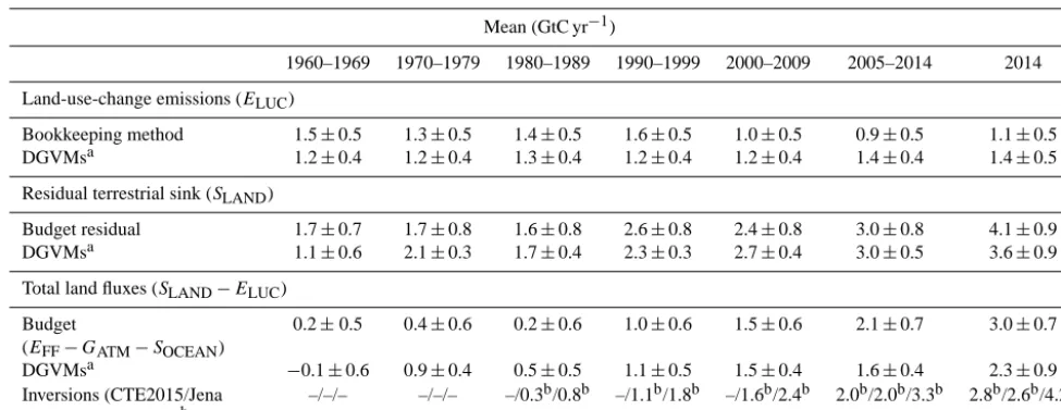
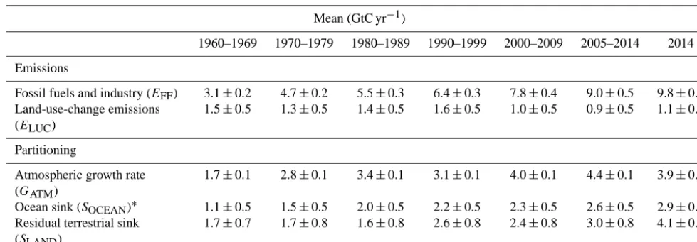
the mean land and ocean fluxes and their variability to estimates from three atmospheric inverse methods for three broad latitude bands. All uncertainties are reported as ±1σ, reflecting the current capacity to charac-terise the annual estimates of each component of the global carbon budget. For the last decade available (2005– 2014),EFFwas 9.0±0.5 GtC yr−1,ELUCwas 0.9±0.5 GtC yr−1,GATMwas 4.4±0.1 GtC yr−1,SOCEANwas
2.6±0.5 GtC yr−1, andSLANDwas 3.0±0.8 GtC yr−1. For the year 2014 alone,EFFgrew to 9.8±0.5 GtC yr−1,
0.6 % above 2013, continuing the growth trend in these emissions, albeit at a slower rate compared to the average growth of 2.2 % yr−1that took place during 2005–2014. Also, for 2014,ELUCwas 1.1±0.5 GtC yr−1,GATM
was 3.9±0.2 GtC yr−1,SOCEANwas 2.9±0.5 GtC yr−1, andSLANDwas 4.1±0.9 GtC yr−1.GATMwas lower in 2014 compared to the past decade (2005–2014), reflecting a largerSLANDfor that year. The global atmospheric CO2concentration reached 397.15±0.10 ppm averaged over 2014. For 2015, preliminary data indicate that the
growth inEFFwill be near or slightly below zero, with a projection of−0.6 [range of−1.6 to+0.5] %, based on national emissions projections for China and the USA, and projections of gross domestic product corrected for recent changes in the carbon intensity of the global economy for the rest of the world. From this
projec-tion ofEFFand assumed constantELUCfor 2015, cumulative emissions of CO2will reach about 555±55 GtC
(2035±205 GtCO2) for 1870–2015, about 75 % fromEFFand 25 % fromELUC. This living data update
docu-ments changes in the methods and data sets used in this new carbon budget compared with previous publications of this data set (Le Quéré et al., 2015, 2014, 2013). All observations presented here can be downloaded from the Carbon Dioxide Information Analysis Center (doi:10.3334/CDIAC/GCP_2015).
1 Introduction
The concentration of carbon dioxide (CO2) in the
atmo-sphere has increased from approximately 277 parts per mil-lion (ppm) in 1750 (Joos and Spahni, 2008), the beginning of the industrial era, to 397.15 ppm in 2014 (Dlugokencky and Tans, 2015). Daily averages went above 400 ppm for the first time at Mauna Loa station in May 2013 (Scripps, 2013). This station holds the longest running record of direct
measurements of atmospheric CO2concentration (Tans and
Keeling, 2014). The global monthly average concentration was above 400 ppm in March through May 2015 for the first time (Dlugokencky and Tans, 2015; Fig. 1), while at Mauna Loa the seasonally corrected monthly average concentration
reached 400 ppm in March 2015 and continued to rise. The atmospheric CO2 increase above pre-industrial levels was,
1960 1970 1980 1990 2000 2010 310
320 330 340 350 360 370 380 390 400 410
Time (yr)
Atmospheric CO
2
concentration (ppm)
Seasonally corrected trend:
Monthly mean:
Scripps Institution of Oceanography (Keeling et al., 1976) NOAA/ESRL (Dlugokencky & Tans, 2015)
NOAA/ESRL
Figure 1. Surface average atmospheric CO2 concentration,
de-seasonalised (ppm). The 1980–2015 monthly data are from NOAA/ESRL (Dlugokencky and Tans, 2015) and are based on an average of direct atmospheric CO2 measurements from
mul-tiple stations in the marine boundary layer (Masarie and Tans, 1995). The 1958–1979 monthly data are from the Scripps Institu-tion of Oceanography, based on an average of direct atmospheric CO2measurements from the Mauna Loa and South Pole stations (Keeling et al., 1976). To take into account the difference of mean CO2between the NOAA/ESRL and the Scripps station networks
used here, the Scripps surface average (from two stations) was har-monised to match the NOAA/ESRL surface average (from multiple stations) by adding the mean difference of 0.542 ppm, calculated here from overlapping data during 1980–2012. The mean seasonal cycle is also shown from 1980.
The global carbon budget presented here refers to the mean, variations, and trends in the perturbation of CO2in the
atmosphere, referenced to the beginning of the industrial era. It quantifies the input of CO2to the atmosphere by emissions
from human activities, the growth of CO2in the atmosphere,
and the resulting changes in the storage of carbon in the land and ocean reservoirs in response to increasing atmospheric CO2levels, climate, and variability, and other anthropogenic
and natural changes (Fig. 2). An understanding of this per-turbation budget over time and the underlying variability and trends of the natural carbon cycle is necessary to understand the response of natural sinks to changes in climate, CO2and
land-use-change drivers, and the permissible emissions for a given climate stabilisation target.
The components of the CO2budget that are reported
annu-ally in this paper include separate estimates for (1) the CO2
emissions from fossil fuel combustion and oxidation and ce-ment production (EFF; GtC yr−1), (2) the CO2emissions
re-sulting from deliberate human activities on land leading to land-use change (ELUC; GtC yr−1), (3) the growth rate of
CO2in the atmosphere (GATM; GtC yr−1), and the uptake of
CO2by the “CO2sinks” in (4) the ocean (SOCEAN; GtC yr−1)
and (5) on land (SLAND; GtC yr−1). The CO2sinks as defined
here include the response of the land and ocean to elevated
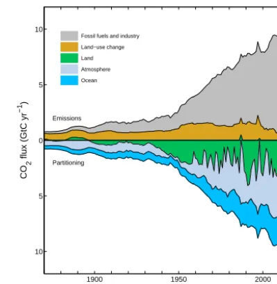
Figure 2.Schematic representation of the overall perturbation of
the global carbon cycle caused by anthropogenic activities, av-eraged globally for the decade 2005–2014. The arrows represent emission from fossil fuels and industry (EFF), emissions from
de-forestation and other land-use change (ELUC), the growth of carbon
in the atmosphere (GATM) and the uptake of carbon by the “sinks”
in the ocean (SOCEAN) and land (SLAND) reservoirs. All fluxes are
in units of GtC yr−1, with uncertainties reported as±1σ(68 % con-fidence that the real value lies within the given interval) as described in the text. This figure is an update of one prepared by the Inter-national Geosphere-Biosphere Programme for the Global Carbon Project (GCP), first presented in Le Quéré (2009).
CO2and changes in climate and other environmental
condi-tions. The global emissions and their partitioning among the atmosphere, ocean, and land are in balance:
EFF+ELUC=GATM+SOCEAN+SLAND. (1) GATM is usually reported in ppm yr−1, which we convert
to units of carbon mass, GtC yr−1, using 1 ppm=2.12 GtC (Ballantyne et al., 2012; Prather et al., 2012; Table 1). We
also include a quantification of EFF by country, computed
with both territorial- and consumption-based accounting (see Sect. 2.1.1).
Equation (1) partly omits two kinds of processes. The first is the net input of CO2to the atmosphere from the chemical
oxidation of reactive carbon-containing gases from sources other than fossil fuels (e.g. fugitive anthropogenic CH4
sions, industrial processes, and changes in biogenic emis-sions from changes in vegetation, fires, wetlands), primar-ily methane (CH4), carbon monoxide (CO), and volatile
or-ganic compounds such as isoprene and terpene. CO emis-sions are currently implicit inEFFwhile anthropogenic CH4
per-Table 1.Factors used to convert carbon in various units (by convention, unit 1=unit 2·conversion).
Unit 1 Unit 2 Conversion Source
GtC (gigatonnes of carbon) ppm (parts per million)a 2.12b Ballantyne et al. (2012)
GtC (gigatonnes of carbon) PgC (petagrams of carbon) 1 SI unit conversion
GtCO2(gigatonnes of carbon dioxide) GtC (gigatonnes of carbon) 3.664 44.01/12.011 in mass equivalent
GtC (gigatonnes of carbon) MtC (megatonnes of carbon) 1000 SI unit conversion
aMeasurements of atmospheric CO
2concentration have units of dry-air mole fraction. “ppm” is an abbreviation for micromole per mole of dry air.bThe use of a factor of 2.12 assumes that all the atmosphere is well mixed within one year. In reality, only the troposphere is well mixed and the growth rate of CO2in the less well-mixed stratosphere is not measured by sites from the NOAA network. Using a factor of 2.12 makes the approximation that the growth rate of CO2in the stratosphere equals that of the troposphere on a yearly basis and reflects the uncertainty in this value.
turbation to carbon cycling in terrestrial freshwaters, estuar-ies, and coastal areas, which modifies lateral fluxes from land
ecosystems to the open ocean; the evasion CO2 flux from
rivers, lakes, and estuaries to the atmosphere; and the net air– sea anthropogenic CO2flux of coastal areas (Regnier et al.,
2013). The inclusion of freshwater fluxes of anthropogenic CO2would affect the estimates of, and partitioning between, SLAND andSOCEAN in Eq. (1) in complementary ways, but would not affect the other terms. These flows are omitted in absence of annual information on the natural versus anthro-pogenic perturbation terms of these loops of the carbon cycle, and they are discussed in Sect. 2.7.
The CO2 budget has been assessed by the
Intergovern-mental Panel on Climate Change (IPCC) in all assessment reports (Ciais et al., 2013; Denman et al., 2007; Prentice et al., 2001; Schimel et al., 1995; Watson et al., 1990), as well as by others (e.g. Ballantyne et al., 2012). These as-sessments included budget estimates for the decades of the 1980s, 1990s (Denman et al., 2007) and, most recently, the period 2002–2011 (Ciais et al., 2013). The IPCC methodol-ogy has been adapted and used by the Global Carbon Project (GCP, www.globalcarbonproject.org), which has coordinated a cooperative community effort for the annual publication of global carbon budgets up to the year 2005 (Raupach et al., 2007; including fossil emissions only), 2006 (Canadell et al., 2007), 2007 (published online; GCP, 2007), 2008 (Le Quéré et al., 2009), 2009 (Friedlingstein et al., 2010), 2010 (Peters et al., 2012b), 2012 (Le Quéré et al., 2013; Peters et al., 2013), 2013 (Le Quéré et al., 2014), and most recently 2014 (Friedlingstein et al., 2014; Le Quéré et al., 2015). The carbon budget year refers to the initial year of publication. Each of these papers updated previous estimates with the latest available information for the entire time series. From 2008, these publications projected fossil fuel emissions for one additional year using the projected world gross domestic product (GDP) and estimated trends in the carbon intensity of the global economy.
We adopt a range of±1 standard deviation (σ) to report the uncertainties in our estimates, representing a likelihood of 68 % that the true value will be within the provided range if the errors have a Gaussian distribution. This choice reflects the difficulty of characterising the uncertainty in the CO2
fluxes between the atmosphere and the ocean and land reser-voirs individually, particularly on an annual basis, as well as the difficulty of updating the CO2emissions from land-use
change. A likelihood of 68 % provides an indication of our current capability to quantify each term and its uncertainty given the available information. For comparison, the Fifth Assessment Report of the IPCC (AR5) generally reported a likelihood of 90 % for large data sets whose uncertainty is well characterised, or for long time intervals less affected by year-to-year variability. Our 68 % uncertainty value is near the 66 % which the IPCC characterises as “likely” for values falling into the±1σinterval. The uncertainties reported here combine statistical analysis of the underlying data and ex-pert judgement of the likelihood of results lying outside this range. The limitations of current information are discussed in the paper and have been examined in detail elsewhere (Bal-lantyne et al., 2015).
All quantities are presented in units of gigatonnes of car-bon (GtC, 1015gC), which is the same as petagrams of car-bon (PgC; Table 1). Units of gigatonnes of CO2 (or billion
tonnes of CO2) used in policy are equal to 3.664 multiplied
by the value in units of GtC.
This paper provides a detailed description of the data sets and methodology used to compute the global carbon bud-get estimates for the period pre-industrial (1750) to 2014 and in more detail for the period 1959 to 2014. We also provide decadal averages starting in 1960 and including the last decade (2005–2014), results for the year 2014, and a
projection of EFF for year 2015. Finally we provide
Carbon Atlas (http://www.globalcarbonatlas.org). With this approach, we aim to provide the highest transparency and traceability in the reporting of CO2, the key driver of climate
change.
2 Methods
Multiple organisations and research groups around the world generated the original measurements and data used to com-plete the global carbon budget. The effort presented here is thus mainly one of synthesis, where results from individual groups are collated, analysed, and evaluated for consistency. We facilitate access to original data with the understanding that primary data sets will be referenced in future work (see Table 2 for how to cite the data sets). Descriptions of the measurements, models, and methodologies follow below and in-depth descriptions of each component are described else-where (e.g. Andres et al., 2012; Houghton et al., 2012).
This is the tenth version of the “global carbon budget” (see Introduction for details) and the fourth revised version of the “global carbon budget living data update”. It is an update of Le Quéré et al. (2015), including data to year 2014 (in-clusive) and a projection for fossil fuel emissions for year 2015. The main changes from Le Quéré et al. (2015) are (1) the use of national emissions forEFFfrom the United
Na-tions Framework Convention on Climate Change (UNFCCC) where available; (2) the projection ofEFFfor 2015 is based
on national emissions projections for China and USA, as well as GDP corrected for recent changes in the carbon intensity of the global economy for the rest of the world; and (3) that we apply minimum criteria of realism to select ocean data products and process models. The main methodological dif-ferences between annual carbon budgets are summarised in Table 3.
2.1 CO2emissions from fossil fuels and industry (EFF) 2.1.1 Emissions from fossil fuels and industry and their
uncertainty
The calculation of global and national CO2emissions from
fossil fuels, including gas flaring and cement production (EFF), relies primarily on energy consumption data, specif-ically data on hydrocarbon fuels, collated and archived by several organisations (Andres et al., 2012). These include the Carbon Dioxide Information Analysis Center (CDIAC), the International Energy Agency (IEA), the United Nations (UN), the United States Department of Energy (DoE) En-ergy Information Administration (EIA), and more recently also the Planbureau voor de Leefomgeving (PBL) Nether-lands Environmental Assessment Agency. Where available, we use national emissions estimated by the countries them-selves and reported to the UNFCCC for the period 1990– 2012 (42 countries). We assume that national emissions re-ported to the UNFCCC are the most accurate because
na-tional experts have access to addina-tional and country-specific information, and because these emission estimates are peri-odically audited for each country through an established in-ternational methodology overseen by the UNFCCC. We also use global and national emissions estimated by CDIAC (Bo-den et al., 2013). The CDIAC emission estimates are the only data set that extends back in time to 1751 with consistent and well-documented emissions from fossil fuels, cement pro-duction, and gas flaring for all countries and their uncertainty (Andres et al., 2014, 2012, 1999); this makes the data set a unique resource for research of the carbon cycle during the fossil fuel era.
The global emissions presented here are from CDIAC’s analysis, which provides an internally consistent global esti-mate including bunker fuels, minimising the effects of lower-quality energy trade data. Thus the comparison of global emissions with previous annual carbon budgets is not influ-enced by the use of data from UNFCCC national reports.
During the period 1959–2011, the emissions from fossil fuels estimated by CDIAC are based primarily on energy data provided by the UN Statistics Division (UN, 2014a, b; Ta-ble 4). When necessary, fuel masses/volumes are converted to fuel energy content using coefficients provided by the UN and then to CO2emissions using conversion factors that take
into account the relationship between carbon content and en-ergy (heat) content of the different fuel types (coal, oil, gas, gas flaring) and the combustion efficiency (to account, for example, for soot left in the combustor or fuel otherwise lost or discharged without oxidation). Most data on energy consumption and fuel quality (carbon content and heat con-tent) are available at the country level (UN, 2014a). In gen-eral, CO2emissions for equivalent primary energy
consump-tion are about 30 % higher for coal compared to oil, and 70 % higher for coal compared to natural gas (Marland et al., 2007). All estimated fossil fuel emissions are based on the mass flows of carbon and assume that the fossil carbon emitted as CO or CH4will soon be oxidised to CO2in the
at-mosphere and can be accounted for with CO2emissions (see
Sect. 2.7).
Our emissions totals for the UNFCCC-reporting countries were recorded as in the UNFCCC submissions, which have a slightly larger system boundary than CDIAC. Additional emissions come from carbonates other than in cement manu-facture, and thus UNFCCC totals will be slightly higher than CDIAC totals in general, although there are multiple sources for differences. We use the CDIAC method to report emis-sions by fuel type (e.g. all coal oxidation is reported under “coal”, regardless of whether oxidation results from combus-tion as an energy source), which differs slightly from UN-FCCC.
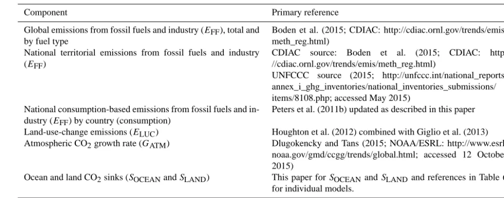
en-Table 2.How to cite the individual components of the global carbon budget presented here.
Component Primary reference
Global emissions from fossil fuels and industry (EFF), total and
by fuel type
Boden et al. (2015; CDIAC: http://cdiac.ornl.gov/trends/emis/ meth_reg.html)
National territorial emissions from fossil fuels and industry (EFF)
CDIAC source: Boden et al. (2015; CDIAC: http:
//cdiac.ornl.gov/trends/emis/meth_reg.html)
UNFCCC source (2015; http://unfccc.int/national_reports/ annex_i_ghg_inventories/national_inventories_submissions/ items/8108.php; accessed May 2015)
National consumption-based emissions from fossil fuels and in-dustry (EFF) by country (consumption)
Peters et al. (2011b) updated as described in this paper
Land-use-change emissions (ELUC) Houghton et al. (2012) combined with Giglio et al. (2013)
Atmospheric CO2growth rate (GATM) Dlugokencky and Tans (2015; NOAA/ESRL: http://www.esrl.
noaa.gov/gmd/ccgg/trends/global.html; accessed 12 October 2015)
Ocean and land CO2sinks (SOCEANandSLAND) This paper forSOCEAN andSLANDand references in Table 6
for individual models.
ergy consumption (coal, oil, gas) for 2013–2014 to the UN-FCCC national emissions in 2012, and for 2012–2014 for the CDIAC national and global emissions in 2011 (BP, 2015). BP’s sources for energy statistics overlap with those of the UN data, but are compiled more rapidly from about 70 coun-tries covering about 96 % of global emissions. We use the BP values only for the year-to-year rate of change, because the rates of change are less uncertain than the absolute values and we wish to avoid discontinuities in the time series when linking the UN-based data with the BP data. These prelimi-nary estimates are replaced by the more complete UNFCCC or CDIAC data based on UN statistics when they become available. Past experience and work by others (Andres et al., 2014; Myhre et al., 2009) show that projections based on the BP rate of change are within the uncertainty provided (see Sect. 3.2 and the Supplement from Peters et al., 2013).
Estimates of emissions from cement production by CDIAC are based on data on growth rates of cement pro-duction from the US Geological Survey up to year 2013 (van Oss, 2013), and up to 2014 for the top 18 countries (representing 85 % of global production; USGS, 2015). For countries without data in 2014 we use the 2013 values (zero growth). Some fraction of the CaO and MgO in cement is re-turned to the carbonate form during cement weathering, but this is generally regarded to be small and is ignored here.
Estimates of emissions from gas flaring by CDIAC are cal-culated in a similar manner to those from solid, liquid, and gaseous fuels, and rely on the UN Energy Statistics to supply the amount of flared or vented fuel. For emission years 2012– 2014, flaring is assumed constant from 2011 (emission year) UN-based data. The basic data on gas flaring report atmo-spheric losses during petroleum production and processing that have large uncertainty and do not distinguish between gas that is flared as CO2 or vented as CH4. Fugitive
emis-sions of CH4 from the so-called upstream sector (e.g. coal
mining and natural gas distribution) are not included in the accounts of CO2emissions except to the extent that they are
captured in the UN energy data and counted as gas “flared or lost”.
The published CDIAC data set includes 250 countries and regions. This expanded list includes countries that no longer exist, such as the USSR and East Pakistan. For the carbon budget, we reduce the list to 216 countries by reallocating emissions to the currently defined territories. This involved both aggregation and disaggregation, and does not change global emissions. Examples of aggregation include merging East and West Germany to the currently defined Germany. Examples of disaggregation include reallocating the emis-sions from former USSR to the resulting independent coun-tries. For disaggregation, we use the emission shares when the current territory first appeared. The disaggregated esti-mates should be treated with care when examining countries’ emissions trends prior to their disaggregation. For the most recent years, 2012–2014, the BP statistics are more aggre-gated, but we retain the detail of CDIAC by applying the growth rates of each aggregated region in the BP data set to its constituent individual countries in CDIAC.
Estimates of CO2emissions show that the global total of
solvents, lubricants, feedstocks), and changes in stock (An-dres et al., 2012).
The uncertainty of the annual emissions from fossil fuels and industry for the globe has been estimated at±5 % (scaled down from the published±10 % at±2σ to the use of±1σ
bounds reported here; Andres et al., 2012). This is consis-tent with a more detailed recent analysis of uncertainty of
±8.4 % at ±2σ (Andres et al., 2014) and at the high end of the range of±5–10 % at±2σ reported by Ballantyne et al. (2015). This includes an assessment of uncertainties in the amounts of fuel consumed, the carbon and heat contents of fuels, and the combustion efficiency. While in the budget we consider a fixed uncertainty of±5 % for all years, in reality the uncertainty, as a percentage of the emissions, is grow-ing with time because of the larger share of global emissions from non-Annex B countries (emerging economies and de-veloping countries) with less precise statistical systems (Mar-land et al., 2009). For example, the uncertainty in Chinese emissions has been estimated at around ±10 % (for ±1σ; Gregg et al., 2008), and important potential biases have been identified that suggest China’s emissions could be overes-timated in published studies (Liu et al., 2015). Generally, emissions from mature economies with good statistical bases have an uncertainty of only a few percent (Marland, 2008). Further research is needed before we can quantify the time evolution of the uncertainty and its temporal error correla-tion structure. We note that, even if they are presented as 1σ
estimates, uncertainties in emissions are likely to be mainly country-specific systematic errors related to underlying bi-ases of energy statistics and to the accounting method used by each country. We assign a medium confidence to the re-sults presented here because they are based on indirect esti-mates of emissions using energy data (Durant et al., 2010). There is only limited and indirect evidence for emissions, although there is a high agreement among the available es-timates within the given uncertainty (Andres et al., 2014, 2012), and emission estimates are consistent with a range of other observations (Ciais et al., 2013), even though their re-gional and national partitioning is more uncertain (Francey et al., 2013).
2.1.2 Emissions embodied in goods and services
National emission inventories take a territorial (production) perspective and “include greenhouse gas emissions and re-movals taking place within national territory and offshore areas over which the country has jurisdiction” (Rypdal et al., 2006). That is, emissions are allocated to the country where and when the emissions actually occur. The territo-rial emission inventory of an individual country does not in-clude the emissions from the production of goods and ser-vices produced in other countries (e.g. food and clothes) that are used for consumption. Consumption-based emission in-ventories for an individual country constitute another attri-bution point of view that allocates global emissions to
prod-ucts that are consumed within a country, and are conceptually calculated as the territorial emissions minus the “embedded” territorial emissions to produce exported products plus the emissions in other countries to produce imported products (consumption=territorial−exports+imports). The differ-ence between the territorial- and consumption-based emis-sion inventories is the net transfer (exports minus imports) of emissions from the production of internationally traded prod-ucts. Consumption-based emission attribution results (e.g. Davis and Caldeira, 2010) provide additional information to territorial-based emissions that can be used to understand emission drivers (Hertwich and Peters, 2009), quantify emis-sion (virtual) transfers by the trade of products between countries (Peters et al., 2011b), and potentially design more effective and efficient climate policy (Peters and Hertwich, 2008).
We estimate consumption-based emissions by enumerat-ing the global supply chain usenumerat-ing a global model of the eco-nomic relationships between ecoeco-nomic sectors within and between every country (Andrew and Peters, 2013; Peters et al., 2011a). Due to availability of the input data, detailed es-timates are made for the years 1997, 2001, 2004, 2007, and 2011 (using the methodology of Peters et al., 2011b) using economic and trade data from the Global Trade and Analysis Project version 9 (GTAP; Narayanan et al., 2015). The results cover 57 sectors and 140 countries and regions. The results are extended into an annual time series from 1990 to the lat-est year of the fossil fuel emissions or GDP data (2013 in this budget), using GDP data by expenditure in current exchange rate of US dollars (USD; from the UN National Accounts Main Aggregates Database; UN, 2014c) and time series of trade data from GTAP (based on the methodology in Peters et al., 2011b).
We estimate the sector-level CO2emissions using our own
calculations based on the GTAP data and methodology, in-clude flaring and cement emissions from CDIAC, and then scale the national totals (excluding bunker fuels) to match the CDIAC estimates from the most recent carbon budget. We do not include international transportation in our estimates of national totals, but we do include them in the global to-tal. The time series of trade data provided by GTAP covers the period 1995–2011 and our methodology uses the trade shares as this data set. For the period 1990–1994 we assume the trade shares of 1995, while for 2012 and 2013 we assume the trade shares of 2011.
to decrease with aggregation (Peters et al., 2011b; e.g. the results for Annex B countries will be more accurate than the sector results for an individual country).
The consumption-based emissions attribution method con-siders the CO2emitted to the atmosphere in the production
of products, but not the trade in fossil fuels (coal, oil, gas). It is also possible to account for the carbon trade in fossil fuels (Davis et al., 2011), but we do not present those data here. Peters et al. (2012a) additionally considered trade in biomass.
The consumption data do not modify the global average terms in Eq. (1) but are relevant to the anthropogenic car-bon cycle as they reflect the trade-driven movement of emis-sions across the Earth’s surface in response to human activ-ities. Furthermore, if national and international climate poli-cies continue to develop in an unharmonised way, then the trends reflected in these data will need to be accommodated by those developing policies.
2.1.3 Growth rate in emissions
We report the annual growth rate in emissions for adjacent years (in percent per year) by calculating the difference be-tween the two years and then comparing to the emissions
in the first year:
E
FF(t0+1)−EFF(t0)
EFF(t0)
×100 % yr−1. This is the simplest method to characterise a 1-year growth compared to the previous year and is widely used. We apply a leap-year adjustment to ensure valid interpretations of annual growth rates. This would affect the growth rate by about 0.3 % yr−1 (1/365) and causes growth rates to go up approximately 0.3 % if the first year is a leap year and down 0.3 % if the second year is a leap year.
The relative growth rate of EFF over time periods of
greater than 1 year can be re-written using its logarithm equivalent as follows:
1
EFF
dEFF
dt =
d(lnEFF)
dt . (2)
Here we calculate relative growth rates in emissions for multi-year periods (e.g. a decade) by fitting a linear trend to ln(EFF) in Eq. (2), reported in percent per year. We fit
the logarithm of EFF rather than EFFdirectly because this
method ensures that computed growth rates satisfy Eq. (6). This method differs from previous papers (Canadell et al., 2007; Le Quéré et al., 2009; Raupach et al., 2007) that com-puted the fit toEFFand divided by averageEFFdirectly, but the difference is very small (<0.05 %) in the case ofEFF.
2.1.4 Emissions projections
Energy statistics from BP are normally available around June for the previous year. To gain insight into emission trends for the current year (2015), we provide an assessment of global
emissions forEFF by combining individual assessments of
emissions for China and the USA (the two biggest emitting countries), as well as the rest of the world.
We specifically estimate emissions in China because the evidence suggests a departure from the long-term trends in the carbon intensity of the economy used in emissions pro-jections in previous global carbon budgets (e.g. Le Quéré et al., 2015), resulting from significant drops in industrial pro-duction against continued growth in economic output. This departure could be temporary (Jackson et al., 2015). Our 2015 estimate for China uses (1) apparent consumption of coal for January to August estimated using production data from the National Bureau of Statistics (2015b), imports and exports of coal from China Customs Statistics (General Ad-ministration of Customs of the People’s Republic of China, 2015a, b), and from partial data on stock changes from indus-try sources (China Coal Indusindus-try Association, 2015; China Coal Resource, 2015); (2) apparent consumption of oil and gas for January to June from the National Energy Admin-istration (2015); and (3) production of cement reported for January to August (National Bureau of Statistics of China, 2015b). Using these data, we estimate the change in emis-sions for the corresponding months in 2015 compared to 2014 assuming constant emission factors. We then assume that the relative changes during the first 6–8 months will per-sist throughout the year. The main sources of uncertainty are from the incomplete data on stock changes, the carbon con-tent of coal, and the assumption of persiscon-tent behaviour for the rest of 2015. These are discussed further in Sect. 3.2.1. We tested our new method using data available in Octo-ber 2014 to make a 2014 projection of coal consumption and cement production, both of which changed substantially in 2014. For the apparent consumption of coal we would have projected a change of−3.2 % in coal use for 2014, compared to−2.9 % reported by the National Bureau of Statistics of China in February 2015, while for the production of cement
we would have projected a change of+3.5 %, compared to
a realised change of+2.3 %. In both cases, the projection is consistent with the sign of the realised change. This new method should be more reliable as it is based on actual data, even if they are preliminary. Note that the growth rates we project for China are unaffected by recent upwards revisions of Chinese energy consumption statistics (National Bureau of Statistics of China, 2015a), as all data used here dates from after the revised period. The revisions do, however, affect the absolute value of the time series up to 2013, and hence the absolute value for 2015 extrapolated from that time series using projected growth rates. Further, because the revisions will increase China’s share of total global emissions, the pro-jected growth rate of global emissions will also be affected slightly. This effect is discussed in the Results section.
ex-penditures by fuel type, energy markets, policies, and other effects. We combine this with our estimate of emissions from cement production using the monthly US cement data from USGS for January–July, assuming changes in cement pro-duction over the first 7 months apply throughout the year. We estimate an uncertainty range using the revisions of historical October forecasts made by the EIA 1 year later. These revi-sions were less than 2 % during 2009–2014 (when a forecast was done), except for 2011, when it was−4.0 %. We thus use a conservative uncertainty range of −4.0 to+1.8 % around the central forecast.
For the rest of the world, we use the close relationship between the growth in GDP and the growth in emissions (Raupach et al., 2007) to project emissions for the current year. This is based on the so-called Kaya identity (also called IPAT identity, the acronym standing for human im-pact (I) on the environment, which is equal to the prod-uct of population (P), affluence (A), and technology (T)), whereby EFF (GtC yr−1) is decomposed by the product of
GDP (USD yr−1) and the fossil fuel carbon intensity of the economy (IFF; GtC USD−1) as follows:
EFF=GDP×IFF. (3)
Such product-rule decomposition identities imply that the relative growth rates of the multiplied quantities are additive. Taking a time derivative of Eq. (3) gives
dEFF
dt =
d(GDP×IFF)
dt (4)
and applying the rules of calculus
dEFF
dt =
dGDP
dt ×IFF+GDP×
dIFF
dt . (5)
Finally, dividing Eq. (5) by (3) gives
1
EFF
dEFF
dt =
1 GDP
dGDP
dt +
1
IFF
dIFF
dt , (6)
where the left-hand term is the relative growth rate of EFF
and the right-hand terms are the relative growth rates of GDP andIFF, respectively, which can simply be added linearly to give overall growth rate. The growth rates are reported in per-cent by multiplying each term by 100 %. As preliminary esti-mates of annual change in GDP are made well before the end of a calendar year, making assumptions on the growth rate of
IFF allows us to make projections of the annual change in
CO2 emissions well before the end of a calendar year. The IFFis based on GDP in constant PPP (purchasing power par-ity) from the IEA up to 2012 (IEA/OECD, 2014) and ex-tended using the IMF growth rates for 2013 and 2014 (IMF, 2015). Experience of the past year has highlighted that the interannual variability inIFFis the largest source of
uncer-tainty in the GDP-based emissions projections. We thus use the standard deviation of the annualIFFfor the period 2005–
2014 as a measure of uncertainty, reflecting ±1σ as in the
rest of the carbon budget. This is±1.4 % yr−1for the rest of
the world (global emissions minus China and USA). The 2015 projection for the world is made of the sum of the projections for China, the USA, and the rest of the world. The uncertainty is added quadratically among the three re-gions. The uncertainty here reflects the best of our expert opinion.
2.2 CO2emissions from land use, land-use change, and forestry (ELUC)
Land-use-change emissions reported here (ELUC) include
CO2fluxes from deforestation, afforestation, logging (forest
degradation and harvest activity), shifting cultivation (cycle of cutting forest for agriculture and then abandoning), and regrowth of forests following wood harvest or abandonment of agriculture. Only some land management activities (Ta-ble 5) are included in our land-use-change emissions esti-mates (e.g. emissions or sinks related to management and management changes of established pasture and croplands are not included). Some of these activities lead to emissions of CO2 to the atmosphere, while others lead to CO2 sinks. ELUC is the net sum of all anthropogenic activities
consid-ered. Our annual estimate for 1959–2010 is from a book-keeping method (Sect. 2.2.1) primarily based on net forest area change and biomass data from the Forest Resource As-sessment (FRA) of the Food and Agriculture Organization (FAO), which is only available at intervals of 5 years. We use the FAO FRA 2010 here (Houghton et al., 2012). Interannual variability in emissions due to deforestation and degradation has been coarsely estimated from satellite-based fire activity in tropical forest areas (Sect. 2.2.2; Giglio et al., 2013; van der Werf et al., 2010). The bookkeeping method is used to quantify theELUCover the time period of the available data,
and the satellite-based deforestation fire information to incor-porate interannual variability (ELUCflux annual anomalies)
from tropical deforestation fires. The satellite-based defor-estation and degradation fire emissions estimates are avail-able for years 1997–2014. We calculate the global annual anomaly in deforestation and degradation fire emissions in tropical forest regions for each year, compared to the 1997–
2010 period, and add this annual flux anomaly to theELUC
estimated using the bookkeeping method that is available up to 2010 only and assumed constant at the 2010 value during the period 2011–2014. We thus assume that all land manage-ment activities apart from deforestation and degradation do not vary significantly on a year-to-year basis. Other sources of interannual variability (e.g. the impact of climate variabil-ity on regrowth fluxes) are accounted for inSLAND. In
ad-dition, we use results from dynamic global vegetation mod-els (see Sect. 2.2.3 and Table 6) that calculate net land-use-change CO2emissions in response to land-cover-change
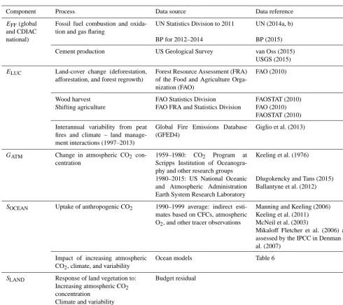
Table 4.Data sources used to compute each component of the global carbon budget. National emissions from UNFCCC are provided directly and thus no additional data sources need citing in this table.
Component Process Data source Data reference
EFF(global
and CDIAC
Fossil fuel combustion and oxida-tion and gas flaring
UN Statistics Division to 2011 UN (2014a, b)
national) BP for 2012–2014 BP (2015)
Cement production US Geological Survey van Oss (2015)
USGS (2015)
ELUC Land-cover change (deforestation,
afforestation, and forest regrowth)
Forest Resource Assessment (FRA) of the Food and Agriculture Orga-nization (FAO)
FAO (2010)
Wood harvest FAO Statistics Division FAOSTAT (2010)
Shifting agriculture FAO FRA and Statistics Division FAO (2010)
FAOSTAT (2010)
Interannual variability from peat fires and climate – land manage-ment interactions (1997–2013)
Global Fire Emissions Database (GFED4)
Giglio et al. (2013)
GATM Change in atmospheric CO2
con-centration
1959–1980: CO2 Program at
Scripps Institution of Oceanogra-phy and other research groups
Keeling et al. (1976)
1980–2015: US National Oceanic and Atmospheric Administration Earth System Research Laboratory
Dlugokencky and Tans (2015) Ballantyne et al. (2012)
SOCEAN Uptake of anthropogenic CO2 1990–1999 average: indirect
esti-mates based on CFCs, atmospheric O2, and other tracer observations
Manning and Keeling (2006) Keeling et al. (2011) McNeil et al. (2003)
Mikaloff Fletcher et al. (2006) as assessed by the IPCC in Denman et al. (2007)
Impact of increasing atmospheric CO2, climate, and variability
Ocean models Table 6
SLAND Response of land vegetation to:
Increasing atmospheric CO2
concentration
Climate and variability Other environmental changes
Budget residual
our understanding. The three methods are described below, and differences are discussed in Sect. 3.2.
2.2.1 Bookkeeping method
Land-use-change CO2 emissions are calculated by a
book-keeping method approach (Houghton, 2003) that keeps track of the carbon stored in vegetation and soils before deestation or other land-use change, and the changes in for-est age classes, or cohorts, of disturbed lands after land-use change, including possible forest regrowth after deforesta-tion. The approach tracks the CO2emitted to the atmosphere
immediately during deforestation, and over time due to the follow-up decay of soil and vegetation carbon in different
pools, including wood product pools after logging and defor-estation. It also tracks the regrowth of vegetation and asso-ciated build-up of soil carbon pools after land-use change. It considers transitions between forests, pastures, and cropland; shifting cultivation; degradation of forests where a fraction of the trees is removed; abandonment of agricultural land; and forest management such as wood harvest and, in the USA, fire management. In addition to tracking logging debris on the forest floor, the bookkeeping method tracks the fate of carbon contained in harvested wood products that is even-tually emitted back to the atmosphere as CO2, although a
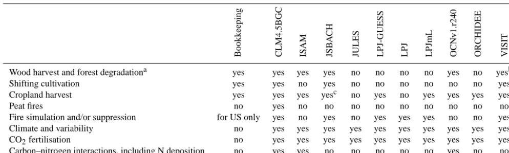
Table 5.Comparison of the processes included in theELUCof the global carbon budget and the DGVMs. See Table 6 for model references.
All models include deforestation and forest regrowth after abandonment of agriculture (or from afforestation activities on agricultural land).
Bookk
eeping
CLM4.5BGC ISAM JSB
A
CH
JULES LPJ-GUESS LPJ LPJmL OCNv1.r240 ORCHIDEE VISIT
Wood harvest and forest degradationa yes yes yes yes no no no no yes no yesb
Shifting cultivation yes yes no yes no no no no no no yes
Cropland harvest yes yes yes yesc no yes no yes yes yes yes
Peat fires no yes no no no no no no no no no
Fire simulation and/or suppression for US only yes no yes no yes yes yes no no yes
Climate and variability no yes yes yes yes yes yes yes yes yes yes
CO2fertilisation no yes yes yes yes yes yes yes yes yes yes
Carbon–nitrogen interactions, including N deposition no yes yes no no no no no yes no no
aRefers to the routine harvest of established managed forests rather than pools of harvested products.bWood stems are harvested according to the land-use data.cCarbon from crop
harvest is entirely transferred into the litter pools.
fuelwood is assumed burnt in the year of harvest (1.0 yr−1). Pulp and paper products are oxidised at a rate of 0.1 yr−1,
timber is assumed to be oxidised at a rate of 0.01 yr−1, and
elemental carbon decays at 0.001 yr−1. The general
assump-tions about partitioning wood products among these pools are based on national harvest data (Houghton, 2003).
The primary land-cover-change and biomass data for the bookkeeping method analysis is the Forest Resource As-sessment of the FAO, which provides statistics on forest-cover change and management at intervals of 5 years (FAO, 2010). The data are based on countries’ self-reporting, some of which integrates satellite data in more recent assessments (Table 4). Changes in land cover other than forest are based on annual, national changes in cropland and pasture areas reported by the FAO Statistics Division (FAOSTAT, 2010). Land-use-change country data are aggregated by regions. The carbon stocks on land (biomass and soils), and their re-sponse functions subsequent to land-use change, are based on FAO data averages per land-cover type, per biome, and per region. Similar results were obtained using forest biomass carbon density based on satellite data (Baccini et al., 2012). The bookkeeping method does not include land ecosystems’ transient response to changes in climate, atmospheric CO2,
and other environmental factors, but the growth/decay curves are based on contemporary data that will implicitly reflect the effects of CO2and climate at that time. Results from the
bookkeeping method are available from 1850 to 2010.
2.2.2 Fire-based interannual variability inELUC
Land-use-change-associated CO2emissions calculated from
satellite-based fire activity in tropical forest areas (van der Werf et al., 2010) provide information on emissions due to tropical deforestation and degradation that are complemen-tary to the bookkeeping approach. They do not provide a di-rect estimate ofELUCas they do not include non-combustion
processes such as respiration, wood harvest, wood products, or forest regrowth. Legacy emissions such as decomposi-tion from on-ground debris and soils are not included in this method either. However, fire estimates provide some in-sight into the year-to-year variations in the subcomponent of the total ELUC flux that result from immediate CO2
emis-sions during deforestation caused, for example, by the in-teractions between climate and human activity (e.g. there is more burning and clearing of forests in dry years) that are not represented by other methods. The “deforestation fire emis-sions” assume an important role of fire in removing biomass in the deforestation process, and thus can be used to infer gross instantaneous CO2emissions from deforestation using
satellite-derived data on fire activity in regions with active deforestation. The method requires information on the frac-tion of total area burned associated with deforestafrac-tion ver-sus other types of fires, and this information can be merged with information on biomass stocks and the fraction of the biomass lost in a deforestation fire to estimate CO2
emis-sions. The satellite-based deforestation fire emissions are limited to the tropics, where fires result mainly from human activities. Tropical deforestation is the largest and most vari-able single contributor toELUC.
differ-ent assumptions to compute decay functions compared to the bookkeeping method, and does not include historical emis-sions or regrowth from land-use change prior to the avail-ability of satellite data. Comparing coincident CO emissions and their atmospheric fate with satellite-derived CO concen-trations allows for some validation of this approach (e.g. van der Werf et al., 2008). Results from the fire-based method to estimate land-use-change emissions anomalies added to the
bookkeeping mean ELUC estimate are available from 1997
to 2014. Our combination of land-use-change CO2emissions
where the variability in annual CO2deforestation emissions
is diagnosed from fires assumes that year-to-year variability is dominated by variability in deforestation.
2.2.3 Dynamic global vegetation models (DGVMs)
Land-use-change CO2 emissions have been estimated
us-ing an ensemble of 10 DGVMs. New model experiments up to year 2014 have been coordinated by the project “Trends and drivers of the regional-scale sources and sinks of carbon dioxide” (TRENDY; Sitch et al., 2015). We use only models that have estimated land-use-change CO2emissions and the
terrestrial residual sink following the TRENDY protocol (see Sect. 2.5.2), thus providing better consistency in the assess-ment of the causes of carbon fluxes on land. Models use their latest configurations, summarised in Tables 5 and 6.
The DGVMs were forced with historical changes in land-cover distribution, climate, atmospheric CO2concentration,
and N deposition. As further described below, each historical DGVM simulation was repeated with a time-invariant pre-industrial land-cover distribution, allowing for estimation of, by difference with the first simulation, the dynamic evolution of biomass and soil carbon pools in response to prescribed land-cover change. All DGVMs represent deforestation and (to some extent) regrowth, the most important components ofELUC, but they do not represent all processes resulting
di-rectly from human activities on land (Table 5). DGVMs rep-resent processes of vegetation growth and mortality, as well as decomposition of dead organic matter associated with nat-ural cycles, and include the vegetation and soil carbon re-sponse to increasing atmospheric CO2levels and to climate
variability and change. In addition, three models explicitly simulate the coupling of C and N cycles and account for at-mospheric N deposition (Table 5). The DGVMs are indepen-dent of the other budget terms except for their use of atmo-spheric CO2concentration to calculate the fertilisation effect
of CO2on primary production.
The DGVMs used a consistent land-use-change data set (Hurtt et al., 2011), which provided annual, half-degree, frac-tional data on cropland, pasture, primary vegetation, and sec-ondary vegetation, as well as all underlying transitions be-tween land-use states, including wood harvest and shifting cultivation. This data set used the HYDE (Klein Goldewijk et al., 2011) spatially gridded maps of cropland, pasture, and ice/water fractions of each grid cell as an input. The HYDE
data are based on annual FAO statistics of change in agricul-tural area available to 2012 (FAOSTAT, 2010). For the years 2013 and 2014, the HYDE data were extrapolated by coun-try for pastures and cropland separately based on the trend in agricultural area over the previous 5 years. The HYDE data are independent of the data set used in the bookkeeping method (Houghton, 2003, and updates), which is based pri-marily on forest area change statistics (FAO, 2010). Although the HYDE use-change data set indicates whether land-use changes occur on forested or non-forested land, typi-cally only the changes in agricultural areas are used by the models and are implemented differently within each model (e.g. an increased cropland fraction in a grid cell can either be at the expense of grassland, or forest, the latter resulting in deforestation; land-cover fractions of the non-agricultural land differ between models). Thus the DGVM forest area and forest area change over time is not consistent with the Forest Resource Assessment of the FAO forest area data used for the bookkeeping model to calculateELUC. Similarly,
model-specific assumptions are applied to convert deforested biomass or deforested area, and other forest product pools, into carbon in some models (Table 5).
The DGVM runs were forced by either 6-hourly CRU-NCEP or by monthly CRU temperature, precipitation, and cloud cover fields (transformed into incoming surface radi-ation) based on observations and provided on a 0.5◦×0.5◦ grid and updated to 2014 (CRU TS3.23; Harris et al., 2015). The forcing data include both gridded observations of
cli-mate and global atmospheric CO2, which change over time
(Dlugokencky and Tans, 2015), and N deposition (as used in three models, Table 5; Lamarque et al., 2010).ELUCis di-agnosed in each model by the difference between a model simulation with prescribed historical land-cover change and a simulation with constant, pre-industrial land-cover distribu-tion. Both simulations were driven by changing atmospheric
CO2, climate, and in some models N deposition over the
period 1860–2014. Using the difference between these two
DGVM simulations to diagnose ELUC is not fully
consis-tent with the definition ofELUCin the bookkeeping method
(Gasser and Ciais, 2013; Pongratz et al., 2014). The DGVM
approach to diagnose land-use-change CO2emissions would
be expected to produce systematically higherELUC
emis-sions than the bookkeeping approach if all the parameters of the two approaches were the same, which is not the case (see Sect. 2.5.2).
2.2.4 Other publishedELUCmethods
Other methods have been used to estimate CO2 emissions
from land-use change. We describe some of the most impor-tant methodological differences between the approach used here and other published methods, and for completion, we explain why they are not used in the budget.
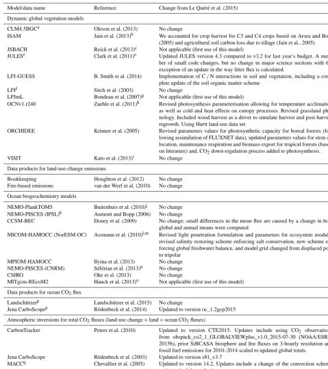
Table 6.References for the process models and data products included in Figs. 6–8.
Model/data name Reference Change from Le Quéré et al. (2015) Dynamic global vegetation models
CLM4.5BGCa Oleson et al. (2013) No change
ISAM Jain et al. (2013)b We accounted for crop harvest for C3 and C4 crops based on Arora and Boer (2005) and agricultural soil carbon loss due to tillage (Jain et al., 2005) JSBACH Reick et al. (2013)c Not applicable (first use of this model)
JULESe Clark et al. (2011)e Updated JULES version 4.3 compared to v3.2 for last year’s budget. A num-ber of small code changes, but no change in major science sections with the exception of an update in the way litter flux is calculated.
LPJ-GUESS B. Smith et al. (2014) Implementation of C/N interactions in soil and vegetation, including a com-plete update of the soil organic matter scheme
LPJf Sitch et al. (2003) No change
LPJmL Bondeau et al. (2007)g Not applicable (first use of this model)
OCNv1.r240 Zaehle et al. (2011)h Revised photosynthesis parameterisation allowing for temperature acclimation as well as cold and heat effects on canopy processes. Revised grassland phe-nology. Included wood harvest as a driver to simulate harvest and post-harvest regrowth. Using Hurtt land-use data set
ORCHIDEE Krinner et al. (2005) Revised parameters values for photosynthetic capacity for boreal forests (fol-lowing assimilation of FLUXNET data), updated parameters values for stem al-location, maintenance respiration and biomass export for tropical forests (based on literature) and, CO2down-regulation process added to photosynthesis.
VISIT Kato et al. (2013)i No change
Data products for land-use-change emissions
Bookkeeping Houghton et al. (2012) No change Fire-based emissions van der Werf et al. (2010) No change Ocean biogeochemistry models
NEMO-PlankTOM5 Buitenhuis et al. (2010)j No change NEMO-PISCES (IPSL)k Aumont and Bopp (2006) No change
CCSM-BEC Doney et al. (2009) No change; small differences in the mean flux are caused by a change in how global and annual means were computed
MICOM-HAMOCC (NorESM-OC) Assmann et al. (2010)l,m Revised light penetration formulation and parameters for ecosystem module, revised salinity restoring scheme enforcing salt conservation, new scheme en-forcing global freshwater balance, and model grid changed from displaced pole to tripolar
MPIOM-HAMOCC Ilyina et al. (2013) No change NEMO-PISCES (CNRM) Séférian et al. (2013)n No change
CSIRO Oke et al. (2013) No change
MITgcm-REcoM2 Hauck et al. (2013)o Not applicable (first use of this model) Data products for ocean CO2flux
Landschützerp Landschützer et al. (2015) No change
Jena CarboScopep Rödenbeck et al. (2014) Updated to version oc_1.2gcp2015 Atmospheric inversions for total CO2fluxes (land-use change+land+ocean CO2fluxes)
CarbonTracker Peters et al. (2010) Updated to version CTE2015. Updates include using CO2 observations from obspack_co2_1_GLOBALVIEWplus_v1.0_2015-07-30 (NOAA/ESRL, 2015b), prior SiBCASA biosphere and fire fluxes on 3-hourly resolution and fossil fuel emissions for 2010–2014 scaled to updated global totals.
Jena CarboScope Rödenbeck et al. (2003) Updated to version s81_v3.7
MACCq Chevallier et al. (2005) Updated to version 14.2. Updates include a change of the convection scheme and a revised data selection.
aCommunity Land Model 4.5.bSee also El-Masri et al. (2013).cSee also Goll et al. (2015).dJoint UK Land Environment Simulator.eSee also Best et al. (2011).fLund–Potsdam–Jena.gThe
LPJmL (Lund–Potsdam–Jena managed Land) version used also includes developments described in Rost et al. (2008; river routing and irrigation), Fader et al. (2010; agricultural management), Biemans et al. (2011; reservoir management), Schaphoff et al. (2013; permafrost and 5 layer hydrology), and Waha et al. (2012; sowing data) (sowing dates).hSee also Zaehle et al. (2010) and
Friend (2010).iSee also Ito and Inatomi (2012).jWith no nutrient restoring below the mixed layer depth.kReferred to as LSCE in previous carbon budgets.lWith updates to the physical model as described in Tjiputra et al. (2013).mFurther information (e.g. physical evaluation) for these models can be found in Danabasoglu et al. (2014).nUsing winds from Atlas et al. (2011).oA few
changes have been applied to the ecosystem model. (1) The constant Fe : C ratio was substituted by a constant Fe : N ratio. (2) A sedimentary iron source was implemented. (3) the following parameters were changed: CHL_N_max=3.78, Fe2N=0.033, deg_CHL_d=0.1, Fe2N_d=0.033, ligandStabConst=200, constantIronSolubility=0.02.pUpdates using SOCATv3 plus new
2012–2014 data.qThe MACCv14.2 CO
2inversion system, initially described by Chevallier et al. (2005), relies on the global tracer transport model LMDZ (see also Supplement of Chevallier,
within models (Gasser and Ciais, 2013; Hansis et al., 2015; Pongratz et al., 2014) as well as between models and other approaches (Houghton et al., 2012; P. Smith et al., 2014). FAO uses the IPCC approach called “Tier 1” (e.g. Tubiello et al., 2015) to produce a “Land use – forest land” estimate from the Forest Resources Assessment data used in the book-keeping method described in Sect. 2.2.1 (MacDicken, 2015). The Tier 1-type method applies a nationally reported mean forest carbon stock change (above and below ground liv-ing biomass) to nationally reported net forest area change, across all forest land combined (planted and natural forests). The methods implicitly assume instantaneous loss or gain of mean forest. Thus the Tier 1 approach provides an estimate of attributable emissions from the process of land-cover change, but it does not distribute these emissions through time. It also captures a fraction of what the global modelling approach considers residual carbon flux (SLAND), it does not consider loss of soil carbon, and there are no legacy fluxes. Land-use fluxes estimated with this method were 0.47 GtC yr−1in 2001–2010 and 0.22 GtC yr−1in 2011–2015 (Federici et al., 2015). This estimate is not directly comparable with ELUC
used here because of the different boundary conditions. Recent advances in satellite data leading to higher-resolution area change data (e.g. Hansen et al., 2013) and estimates of biomass in live vegetation (e.g. Baccini et al., 2012; Saatchi et al., 2011) have led to several satellite-based estimates of CO2emissions due to tropical
deforesta-tion (typically gross loss of forest area; Achard and House, 2015). These include estimates of 1.0 GtC yr−1for 2000 to 2010 (Baccini et al., 2012), 0.8 GtC yr−1 for 2000 to 2005 (Harris et al., 2012), 0.9 GtC yr−1for 2000 to 2010 for net
area change (Achard et al., 2014), and 1.3 GtC yr−12000 to
2010 (Tyukavina et al., 2015). These estimates include be-lowground carbon biomass using a scaling factor. Some esti-mate soil carbon loss, some assume instantaneous emissions, some do not account for regrowth fluxes, and none account for legacy fluxes from land-use change prior to the avail-ability of satellite data. They are mostly estimates of tropi-cal deforestation only, and do not capture regrowth flux after abandonment or planting (Achard and House, 2015). These estimates are also difficult to compare withELUCused here because they do not fully include legacy fluxes and forest re-growth.
2.2.5 Uncertainty assessment forELUC
Differences between the bookkeeping, the addition of fire-based interannual variability to the bookkeeping, and DGVM methods originate from three main sources: the land-cover-change data set, the different approaches used in models, and the different processes represented (Table 5). We examine the results from the 10 DGVMs and of the bookkeeping method to assess the uncertainty inELUC.
The uncertainties in annualELUCestimates are examined
using the standard deviation across models, which averages
0.4 GtC yr−1from 1959 to 2014 (Table 7). The mean of the
multi-modelELUC estimates is consistent with a
combina-tion of the bookkeeping method and fire-based emissions (Le Quéré et al., 2014), with the multi-model mean and bookkeeping method differing by less than 0.5 GtC yr−1over 85 % of the time. Based on this comparison, we assess that an uncertainty of±0.5 GtC yr−1provides a semi-quantitative measure of uncertainty for annual emissions, and reflects our best value judgment that there is at least 68 % chance (±1σ) that the true land-use-change emission lies within the given range, for the range of processes considered here. This is consistent with the uncertainty analysis of Houghton et al. (2012), which partly reflects improvements in data on for-est area change using data, and partly more complete under-standing and representation of processes in models.
The uncertainties in the decadalELUCestimates are also examined using the DGVM ensemble, although they are likely correlated between decades. The correlations between decades come from (1) common biases in system bound-aries (e.g. not counting forest degradation in some models); (2) common definition for the calculation ofELUCfrom the
difference of simulations with and without land-use change (a source of bias vs. the unknown truth); (3) common and uncertain land-cover-change input data which also cause a bias, though if a different input data set is used each decade, decadal fluxes from DGVMs may be partly decorrelated; and (4) model structural errors (e.g. systematic errors in biomass stocks). In addition, errors arising from uncertain DGVM pa-rameter values would be random, but they are not accounted for in this study, since no DGVM provided an ensemble of runs with perturbed parameters.
Prior to 1959, the uncertainty inELUCis taken as±33 %, which is the ratio of uncertainty to mean from the 1960s (Ta-ble 7), the first decade availa(Ta-ble. This ratio is consistent with the mean standard deviation of DGMVs’ land-use-change emissions over 1870–1958 (0.38 GtC) over the multi-model mean (1.1 GtC).
2.3 Atmospheric CO2growth rate (GATM) Global atmospheric CO2growth rate estimates
The atmospheric CO2growth rate is provided by the US
Na-tional Oceanic and Atmospheric Administration Earth Sys-tem Research Laboratory (NOAA/ESRL; Dlugokencky and Tans, 2015), which is updated from Ballantyne et al. (2012). For the 1959–1980 period, the global growth rate is based on
measurements of atmospheric CO2 concentration averaged
from the Mauna Loa and South Pole stations, as observed
by the CO2 Program at Scripps Institution of