www.geosci-model-dev.net/8/3215/2015/ doi:10.5194/gmd-8-3215-2015
© Author(s) 2015. CC Attribution 3.0 License.
An open and extensible framework for spatially explicit land use
change modelling: the lulcc R package
S. Moulds1,2, W. Buytaert1,2, and A. Mijic1
1Department of Civil and Environmental Engineering, Imperial College London, London, UK 2Grantham Institute for Climate Change, Imperial College London, London, UK
Correspondence to: S. Moulds ([email protected])
Received: 12 March 2015 – Published in Geosci. Model Dev. Discuss.: 29 April 2015 Revised: 30 July 2015 – Accepted: 6 September 2015 – Published: 9 October 2015
Abstract. We present the lulcc software package, an object-oriented framework for land use change modelling written in the R programming language. The contribution of the work is to resolve the following limitations associated with the current land use change modelling paradigm: (1) the source code for model implementations is frequently unavailable, severely compromising the reproducibility of scientific re-sults and making it impossible for members of the com-munity to improve or adapt models for their own purposes; (2) ensemble experiments to capture model structural uncer-tainty are difficult because of fundamental differences be-tween implementations of alternative models; and (3) addi-tional software is required because existing applications fre-quently perform only the spatial allocation of change. The package includes a stochastic ordered allocation procedure as well as an implementation of the CLUE-S algorithm. We demonstrate its functionality by simulating land use change at the Plum Island Ecosystems site, using a data set included with the package. It is envisaged that lulcc will enable future model development and comparison within an open environ-ment.
1 Introduction
Spatially explicit land use change models are used to un-derstand and quantify key processes that affect land use and land cover change and simulate past and future change (Veld-kamp and Lambin, 2001; Mas et al., 2014). These mod-els are commonly implemented in compiled languages such as C/C+ + and Fortran and distributed as software pack-ages or extensions to proprietary geographic information
systems such as ArcGIS or Idrisi. As Rosa et al. (2014) pointed out, it is uncommon for the source code of land use change modelling software to be made available (e.g. Ver-burg et al., 2002; Soares-Filho et al., 2002; VerVer-burg and Over-mars, 2009; Schaldach et al., 2011). While it is true that the concepts and algorithms implemented by the software are normally described in scientific journal articles, this fails to ensure the reproducibility of scientific results (Peng, 2011; Morin et al., 2012), even in the hypothetical case of a per-fectly described model (Ince et al., 2012). In addition, run-ning binary versions of software makes it difficult to detect silent faults (faults that change the model output without ob-vious signals), whereas these are more likely to be identi-fied if the source code is open (Cai et al., 2012). Moreover, it forces duplication of work and makes it difficult for members of the scientific community to improve the code or adapt it for their own purposes (Morin et al., 2012; Pebesma et al., 2012; Steiniger and Hunter, 2013). In this paper we describe the development of lulcc, a new R package designed to foster an open approach to land use change science.
methods to validate model output, which could be one reason for the lack of proper validation of models in the literature, as noted by Rosa et al. (2014). The lack of a common inter-face amongst land use change models is problematic for the community because there is widespread uncertainty about the appropriate model form and structure for modelling ap-plications (Verburg et al., 2013). Under these circumstances it is useful to experiment with various models to identify the model that performs best in terms of calibration and vali-dation (Schmitz et al., 2009). Alternatively, ensemble mod-elling may be used to understand the impact of structural un-certainty on model outcomes (Knutti and Sedláˇcek, 2012). However, while some land use change model comparison studies have been carried out (e.g. Pérez-Vega et al., 2012; Mas et al., 2014; Rosa et al., 2014), fundamental differences between models in terms of scale, resolution and model in-puts prevent the widespread use of ensemble land use change predictions (Rosa et al., 2014). As a result, the uncertainty associated with model outcomes is rarely communicated in a formal way, raising questions about the utility of such mod-els (Pontius and Spencer, 2005).
An alternative approach is to develop frameworks that al-low several modelling approaches to be implemented within the same environment. One such application is PCRaster, a free and open-source geographic information system (GIS) that includes additional capabilities for spatially explicit dy-namic modelling (Schmitz et al., 2009). The PCRcalc script-ing language and development environment allows users to build models with native PCRaster operations such as map algebra and neighbourhood functions. Alternatively, the PCRaster application programming interface (API) allows users to extend its functionality in various programming lan-guages using native and external data types (Schmitz et al., 2009). For example, the current version of FALLOW (van Noordwijk, 2002; Mulia et al., 2014), a deductive land use change model, is built using the PCRaster framework. Ter-raME (Carneiro et al., 2013) is a platform to develop mod-els for simulating interactions between society and the envi-ronment. It provides more flexibility than PCRaster because models can be composed of coupled sub-models with var-ious temporal and spatial resolutions (Moreira et al., 2009; Carneiro et al., 2013). The platform is built on the open-source TerraLib geospatial library (Câmara et al., 2008), which handles several spatio-temporal data types, includes an API for coupling the library with R (R Core Team, 2014) to perform spatial statistics, and supports dynamic modelling with cellular automata. The LuccME extension to TerraME includes implementations of CLUE-S and its predecessor, CLUE (Veldkamp and Fresco, 1996; Verburg et al., 1999), written in Lua.
The R environment is a free and open-source implementa-tion of the S programming language, a language designed for programming with data (Chambers, 2008). Although the de-velopment of R is strongly rooted in statistical software and data analysis, it is increasingly used for dynamic simulation
modelling in diverse fields (Petzoldt and Rinke, 2007). Ad-ditionally, in the last decade it has become widely used by the spatial analysis community, largely due to the sp pack-age (Pebesma and Bivand, 2005; Bivand et al., 2013) which unified many alternative approaches for dealing with spa-tial data in R and allowed subsequent package developers to use a common framework for spatial analysis. The raster package (Hijmans, 2014) provides many functions for raster data manipulation commonly associated with GIS software. Building on these capabilities, several R packages have been created for dynamic, spatially explicit ecological modelling (e.g. Petzoldt and Rinke, 2007; Fiske and Chandler, 2011). In addition, two recent land use change models have been writ-ten for the R environment. StocModLCC (Rosa et al., 2013) is a stochastic inductive land use change model for tropical deforestation, while SIMLANDER (Hewitt et al., 2013) is a stochastic cellular automata model to simulate urbanisa-tion. Thus, R is well-suited for spatially explicit land use change modelling. To date, however, R has not been used to develop a framework for land use change model develop-ment and comparison. The remainder of this paper is divided into four sections. First, we discuss the principle design goals of lulcc. We then describe the software and demonstrate its main functionality with an example application to the Plum Island Ecosystems site, using data included with the package. This is followed by a discussion of the strengths and main limitations of the software and approach, as well as areas for future development. Finally, we draw brief conclusions from the project.
2 Design goals
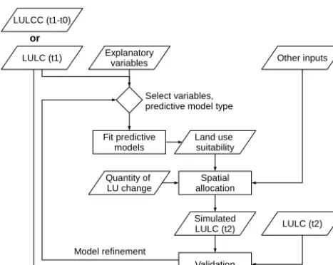
The first design goal of lulcc is to provide a framework that allows users to perform various stages of the modelling pro-cess illustrated by Fig. 1 within the same environment. It therefore includes methods to process and explore model input, fit and evaluate predictive models, allocate land use change spatially, validate the model and visualise model out-puts. This provides many advantages over specialised soft-ware applications. First, it improves efficiency and reduces the likelihood of user errors because intermediate inputs and outputs exist in the same environment (Fiske and Chandler, 2011; Pebesma et al., 2012). Second, it encourages interac-tive model building because separate aspects of the procedure can easily be revisited. Third, it is straightforward to experi-ment with different model set-ups. Finally, and perhaps most importantly, it improves the reproducibility of scientific re-sults because the entire modelling process can be expressed programmatically and be communicated as such with reason-able effort (Pebesma et al., 2012).
LULC (t1) Explanatoryvariables Other inputs
Fit predictive models
Spatial allocation
Validation
LULC (t2) Simulated
LULC (t2) Select variables, predictive model type LULCC (t1-t0)
or
Quantity of LU change
Land use suitability
Model refinement
Figure 1. Diagram showing the general methodology used for
in-ductive land use change modelling applications, adapted from Mas et al. (2014). The input land use/land cover data can be a single categorical map showing the pattern of land use/land cover at one time point (LULC (t1)) or a series of maps showing historical land use/land cover transitions (LULCC (t1–t0)).
extensible framework allowing users to examine the source code, modify it for their own purposes and freely distribute changes to the wider community. The package exploits the openness of the R system, particularly with respect to the package system, which allows developers to contribute code, documentation and data sets in a standardised format to repositories such as the Comprehensive R Archive Network (CRAN) (Pebesma et al., 2012; Claes et al., 2014). As a re-sult of this philosophy, R users have access to a wide range of sophisticated tools for statistical modelling, data manage-ment, spatial analysis and visualisation.
One of the consequences of providing a modelling frame-work in R is that users of the software must become program-mers (Chambers, 2000). We recognise that this represents a different approach to the current practice of providing land use change software packages with graphical user interfaces (GUIs), and acknowledge that for users unfamiliar with pro-gramming it could present a steep learning curve. Therefore, the third design goal is to provide well-documented software that is easy to use and accessible for a users with varying lev-els of programming experience. The package includes com-plete working examples to allow beginners to start using the package immediately from the R command shell, while more advanced users should be able to develop modelling applica-tions as scripts. Furthermore, the package is designed to be extensible so that users can contribute new or existing meth-ods. Similarly, the source code of lulcc is accessible so that users can locate the methods in use and understand algorithm implementations. Acknowledging that many scientists lack any formal training in programming (Joppa et al., 2013; Wil-son et al., 2014), we hope this final goal will ensure the
soft-ware is useful for educational purposes as well as scientific research.
3 Software description
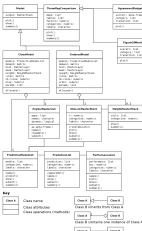
To achieve the design goals, we adopted an object-oriented approach. This provides a formal structure for the modelling framework that allows the various stages of land use change modelling applications to be handled efficiently. Further-more, it encourages the reuse of code because objects can be used multiple times within the same application or across several different applications. It is extensible because it is straightforward to extend existing classes using the concept of inheritance, or create new methods for existing classes. In lulcc we use the S4 class system (Chambers, 1998, 2008), which requires classes and methods to be formally defined. This system is more rigorous than the alternative S3 sys-tem because objects are validated against the class definition when they are created, ensuring that objects behave consis-tently when they are passed to functions and methods. Fig-ure 2 shows the class structFig-ure of lulcc, while Table 1 shows the functions included with the package. Here we describe the main components of lulcc integrated with an example ap-plication for the Plum Island Ecosystems data set. The script used in this paper, including the code used to create the var-ious figures, is supplied with the package as a “demo”. In-structions to obtain the package and run the demo script are provided in the “Code availability” section.
3.1 Data
Table 1. Functions included in the lulcc package.
Function name Description
AgreementBudget Calculate agreement budget (Pontius et al., 2011)
getPredictiveModelInputData Create data.frame with variables required to fit predictive models allocate Perform spatial allocation using various methods
approxExtrapDemand Create a demand scenario by linear extrapolation
compareAUC Compare the area under the curve (AUC) for various predictive models crossTabulate Calculate the contingency table for two categorical raster maps FigureOfMerit Calculate the figure of merit (Pontius et al., 2011)
glmModels Fit multiple glm models NeighbRasterStack Calculate neighbourhood values partition Partition Raster∗map
PredictionList Create a ROCR prediction object for each model in a PredictiveModelList object
PerformanceList Create a ROCR performance object for each prediction object contained in a PredictionList object predict Make predictions using a PredictiveModelList object
randomForestModels Fit multiple random forest models
rpartModels Fit multiple recursive partitioning and regression tree models
resample Resample an ExpVarRasterList object to the parameters of an ObsLulcRasterStack object ThreeMapComparison Calculate three-dimensional contingency tables (Pontius et al., 2011)
total Sum the total number of cells belonging to each class of a categorical raster map
3.2 Data processing
One of the most challenging aspects of land use change mod-elling is to obtain and process the correct input data. Cur-rently, lulcc requires all spatially explicit input data to exist either in the file system, in any of the formats supported by raster, or in the R workspace as raster objects (RasterLayer, RasterStack or RasterBrick). The most fundamental input re-quired by land use change models is an initial map of ob-served land use, which is usually obtained from classified remotely sensed data. This map represents the initial condi-tion for model simulacondi-tions and, for inductive modelling, is used to fit predictive models. Sometimes it is more useful to consider observed land use transitions: in this case an addi-tional map for an earlier time point is required, as shown by Fig. 1. Ideally, two more observed land use maps for sub-sequent time points should be obtained for calibrating and validating the land use change model (Pontius et al., 2004a). The current version of the software only supports categorical land use data, which means that each pixel must belong to exactly one category.
In lulcc, observed land use data are represented by the ObsLulcRasterStack class. In the following code snippet we load the package into the current session, create an ObsLul-cRasterStack object for the Plum Island Ecosystems data set and plot the result (Fig. 3):
> library(lulcc) > data(pie) > obs
<- ObsLulcRasterStack (x=pie,
pattern="lu",
categories=c(1,2,3),
labels=c("Forest","Built","Other"), t=c(0,6,14))
> plot(obs)
The ObsLulcRasterStack object is important to land use change studies in lulcc because it defines the spatial domain of subsequent operations. Thetargument in the construc-tor function specifies the time points associated with the ob-served land use maps. The first time point must always be zero; if additional maps are present they should be associated with time points greater than zero, even in backcast models. In most land use change modelling applications the time step between two time points represents 1 year but there is no re-quirement for this to be the case.
A useful starting point in land use change modelling is to obtain a transition matrix for observed land use maps from two time points to identify the main historical transitions in the study region (Pontius et al., 2004b), which can be used as the basis for further research into the processes driving change. In lulcc we use thecrossTabulatefunction for this purpose:
> crossTabulate(x=obs, times=c(0,14)) Forest Built Other
Forest 44107 4250 656
Built 11 36957 154
Other 1259 2248 23921
The output of this command reveals that for the Plum Is-land Ecosystems site the dominant change between 1985 and 1999 was the conversion from forest to built areas.
Figure 2. Class diagram in the Unified Modeling Language (UML) for lulcc, showing the main classes and methods included in the package.
biophysical and socioeconomic explanatory variables. These may be static, such as elevation or geology, or dynamic, such as maps of population density or road networks. In lulcc these two types of explanatory variable are separated by a simple naming convention, which is explained in detail in the package documentation (see Supplement). Collectively, they are represented by an object of class ExpVarRasterList, which can be created as follows:
> ef <- ExpVarRasterList (x=pie, pattern="ef")
Apart from observed land use and explanatory variables other input maps may be required. The two allocation routines
920000 930000 940000 950000
220000 240000 260000
lu_pie_1985 lu_pie_1991
220000 240000 260000
lu_pie_1999
Forest Built Other
Figure 3. Observed land use maps for the Plum Island Ecosystems site in 1985, 1991 and 1999, created by plotting the ObsLulcRasterStack
object representing the data.
> ef <- resample(ef, obs)
3.3 Predictive modelling
Inductive land use change models relate the pattern of ob-served land use to spatially explicit explanatory variables. Logistic regression is a common type of predictive model used for inductive land use change modelling (e.g. Pon-tius and Schneider, 2001; Verburg et al., 2002). However, there is growing interest in the application of local and non-parametric models (e.g. Tayyebi et al., 2014). One reason why R is attractive for land use change modelling is that it has become the de facto standard for statistical software de-velopment. As a result, lulcc can easily support various pre-dictive modelling techniques by utilising code from existing R packages. Currently, lulcc supports binary logistic sion, available in base R, recursive partitioning and regres-sion trees, provided by the rpart package (Therneau et al., 2014), and random forests, provided by the randomForest package (Liaw and Wiener, 2002).
Parametric models such as logistic regression assume the data to be independent and identically distributed (Overmars et al., 2003). In spatial analysis this assumption is often vi-olated because of spatial autocorrelation, which reduces the information content of an observation because its value can to some extent be predicted by the value of its neighbours (Beale et al., 2010). There is also some evidence that non-parametric models may be affected by spatial autocorrela-tion (Mascaro et al., 2014), even though they do not assume independence. A simple approach to reduce the impact of this phenomenon is to fit predictive models to a random sub-set of the data (e.g. Verburg et al., 2002; Wassenaar et al., 2007; Echeverria et al., 2008). In the following code snip-pet, we create training and testing partitions for the Plum Island Ecosystems data set by performing a stratified ran-dom sample. We do this using the map for 1985 to illus-trate the procedure when only one observed map is available. We then extract the data for the training partition with the getPredictiveModelInputData function and pass the resulting data.frame to the three model fitting functions:
> part <- partition(x=obs[[1]], size=0.1, spatial=TRUE) > train.data
<- getPredictiveModelInputData (obs=obs,
ef=ef,
cells=part[["train"]], t=0)
> forms <- list
(Built~ef_001+ef_002+ef_003, Forest~ef_001+ef_002,
Other~ef_001+ef_002)
> glm.models <- glmModels (formula=forms,
family=binomial, data=train.data, obs=obs)
> rpart.models <- rpartModels (formula=forms,
data=train.data, obs=obs)
> rf.models <- randomForestModels (formula=forms,
data=train.data, obs=obs)
The model fitting functions each return an object of class Pre-dictiveModelList containing a predictive model for each land use type. With these objects, it is straightforward to map the suitability of every pixel in the study region to the various land uses. To do this, we use the genericpredictfunction with some additional functionality from the raster package and plot the resulting RasterStack object (Fig. 4):
> all.data <- as.data.frame
920000 930000 940000 950000
220000 240000 260000
Forest Built
220000 240000 260000
Other
0.0 0.2 0.4 0.6 0.8 1.0
Figure 4. Suitability of pixels in the Plum Island Ecosystems study site to belong to forest, built and other land use classes according to
binary logistic regression models. Elevation and slope are used as explanatory variables for all land uses while built additionally includes distance to built pixels in 1985.
(object=glm.models, newdata=all.data, data.frame=TRUE) > points <- rasterToPoints
(obs[[1]], spatial=TRUE) > probmaps <- SpatialPointsDataFrame
(points, probmaps) > probmaps <- rasterize
(x=probmaps, y=obs[[1]], field=names(probmaps)) > levelplot(probmaps)
In some circumstances it may be appropriate to supply a model with no explanatory variables to an allocation rou-tine. For example, Verburg and Overmars (2009) used such a model for natural and semi-natural vegetation because in their particular case study the selection of pixels for con-version to these land uses was based on the suitability of pixels to agricultural and urban land rather than the suitabil-ity of natural and semi-natural vegetation. In lulcc, this can most easily be achieved by fitting a binary logistic regression model with no explanatory variables. To do this, a formula such asForest∼1should be supplied to theglmModels function.
Methods to evaluate statistical models are provided by the ROCR package (Sing et al., 2005), allowing the user to as-sess model performance using various methods including the receiver operator characteristic (ROC), which is used to mea-sure the performance of models predicting the presence or absence of a phenomenon (Pontius and Parmentier, 2014). It is often summarised by the area under the curve (AUC), where one indicates a perfect fit and 0.5 indicates a purely random fit.
In lulcc we extend the native ROCR classes to better suit our purposes. The prediction and performance classes of ROCR are extended by PredictionList and PerformanceList to handle objects of class PredictiveModelList. In the follow-ing example we evaluate the logistic regression models usfollow-ing the testing partition from the 1985 observed land use map.
Since the Plum Island Ecosystems data set contains three ob-served land use maps, we could also test the predictive mod-els using data from a subsequent time point. The procedure to evaluate several PredictiveModelList objects using these classes is as follows:
> test.data
<- getPredictiveModelInputData (obs=obs,
ef=ef,
cells=part[["test"]]) > glm.pred <- PredictionList
(models=glm.models, newdata=test.data) > glm.perf <- PerformanceList
(pred=glm.pred, measure="rch") > rpart.pred <- PredictionList
(models=rpart.models, newdata=test.data) > rpart.perf <- PerformanceList
(pred=rpart.pred, measure="rch") > rf.pref <- PredictionList
(models=rf.models, newdata=test.data) > rf.perf <- PerformanceList
(pred=rf.pred, measure="rch") > plot(list(glm=glm.perf,
rpart=rpart.perf, rf=rf.perf))
Figure 5 shows the ROC curves for each land use type and for each type of predictive model supported by lulcc. The plots show that binary logistic regression and random forest models perform similarly for all land uses, while regression tree models perform least well.
False Alarms/(False Alarms + Correct Rejections) Hits/(Hits + Misses) 0.0
0.2 0.4 0.6 0.8 1.0
0.0 0.2 0.4 0.6 0.8 1.0 glm: AUC=0.6423 rpart: AUC=0.6222 rf: AUC=0.6117 Forest
0.0 0.2 0.4 0.6 0.8 1.0
glm: AUC=0.9384 rpart: AUC=0.9158 rf: AUC=0.9363 Built
0.0 0.2 0.4 0.6 0.8 1.0 glm: AUC=0.7276 rpart: AUC=0.6458 rf: AUC=0.7074 Other
Figure 5. ROC curves showing the ability of each type of predictive model to simulate the observed pattern of land use in the Plum Island
Ecosystems site in 1985 in the data partition left out of the fitting procedure.
time points. This is only possible if a second observed land use map is available for a subsequent time point. In the fol-lowing code snippet, we perform this type of analysis for the gain of built between 1985 and 1991. First, we create a data partition in which cells not candidate for gain (cells belong-ing to built in 1985) are eliminated. We then assess the ability of the various predictive models to predict the gain of built in this partition:
> part <- rasterToPoints (obs[[1]],
fun=function(x) x != 2, spatial=TRUE)
> test.data
<- getPredictiveModelInputData (obs=obs,
ef=ef, cells=part, t=6)
> glm.pred <- Prediction
(models=glm.models[[2]], newdata=test.data) > glm.perf <- Performance
(pred=glm.pred, measure="rch") > plot(list(glm=glm.perf))
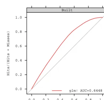
Figure 6 shows the resulting ROC curve.
3.4 Demand
Spatially explicit land use change models are normally driven by non-spatial estimates of either the total number of cells oc-cupied by each category at each time point or the number of transitions among the various categories during each time in-terval. This means regional drivers of land use change, such as population growth and technology, are considered implic-itly (Fuchs et al., 2013). While some models calculate de-mand at each time point based on the spatial configuration of the landscape at the previous time point (e.g. Rosa et al., 2013), it is more common to specify the demand for every
False Alarms/(False Alarms + Correct Rejections)
Hits/(Hits + Misses)
0.0 0.2 0.4 0.6 0.8 1.0
0.0 0.2 0.4 0.6 0.8 1.0
glm: AUC=0.6448 Built
Figure 6. ROC curve showing the ability of the binary logistic
re-gression model fitted on observed land use data from 1985 to predict the gain in built land between 1985 and 1991.
time point at the beginning of the simulation (e.g. Pontius and Schneider, 2001; Verburg et al., 2002; Sohl et al., 2007). In lulcc the way in which demand is specified is unique to in-dividual allocation models. Currently, both allocation models currently included in the package require the total number of cells belonging to each category at every time point to be sup-plied as a matrix or data.frame before running the allocation routine.
> dmd <- approxExtrapDemand (obs=obs, tout=0:14)
In reality we are not usually interested in simulating land use change between two time points for which observed land use data are available. However, doing so is useful for model pat-tern validation, allowing us to test the ability of models to predict the spatial allocation of change given the exact quan-tity of change.
3.5 Allocation
The allocation algorithm in land use change models deter-mines the pixels in which various land use transitions should take place (Verburg et al., 2002). Currently lulcc includes two allocation routines: an implementation of the CLUE-S algorithm and a stochastic ordered procedure based on the algorithm described by Fuchs et al. (2013). Both routines allow the user to optionally provide various decision rules. These are implemented before the main allocation algorithm at each time point and allow the user to incorporate additional knowledge about the study site.
3.5.1 Decision rules
The first decision rule included in lulcc is used to prohibit certain land use transitions. For example, in most situations it is unlikely that urban areas will be converted to agricul-tural land because the initial cost of urban development is high (Verburg et al., 2002). The second rule specifies a min-imum number of time steps before a certain transition is al-lowed, while the third rule specifies a maximum number of time steps after which change is not allowed. These rules are used to control land use transitions that are time dependent, such as the transition from shrubland to closed forest (Ver-burg and Overmars, 2009). The fourth rule prohibits transi-tions to a certain land use in cells that are not within a user-defined neighbourhood of cells already belonging to that land use. This rule is particularly relevant to cases of deforestation or urbanisation.
Within the allocate function the first three decision rules are applied by theallowfunction and the fourth rule is applied by theallowNeighbfunction. For time dependent decision rules, the user should supply a land use history raster map, specifying the length of time each pixel has belonged to the current land use. If this is not supplied, each pixel is assigned a value of one representing one model time step. To apply neighbourhood rules, it is necessary to supply corre-sponding neighbourhood maps to the allocation routine. In lulcc these are represented by theNeighbRasterStack class. Objects of this class are created with the following command:
> w <- matrix
(data=1, nrow=3, ncol=3) > nb <- NeighbRasterStack
(x=obs[[1]], weights=w, categories=c(1,2,3))
Essentially, the allow and allowNeighb functions identify disallowed transitions according to the decision rules and set the suitability of these cells to n/a. These transitions are ignored by the allocation routine. Care should be taken to ensure that after any decision rules are taken into account there are sufficient cells eligible to change in order to meet the specified demand at each time point.
3.5.2 CLUE-S allocation method
The CLUE-S model implements an iterative procedure to meet the specified demand at each time point and handle competition between land uses. The model is summarised briefly here: for a full description see Verburg et al. (2002) and Castella and Verburg (2007). The algorithm in lulcc is based on the description of the model provided by Verburg et al. (2002) only. As a result, for the reasons discussed by Ince et al. (2012), users should not expect to exactly repro-duce the output from the original model implementation.
In the first instance each cell is allocated to the land use with the highest suitability as determined by the predictive models. Whereas the original CLUE-S model is based on bi-nary logistic regression, lulcc allows any predictive model supported by PredictiveModelList to be used. For each land use the algorithm determines whether the allocated area is less than, equal to or greater than the specified demand. If it is less than or greater than demand, the suitability of each pixel in the study region to the land use in question will be in-creased or dein-creased, respectively, by an amount depending on the difference between the allocated area and specified de-mand. If the allocated area equals demand, the suitability is left unchanged. This procedure is repeated until the demand for all land uses, within a user-defined tolerance, is met. At each iteration the original model perturbs the suitability of each pixel to the various land uses in order to limit the influ-ence of nominal differinflu-ences in land use suitability on the final model solution. This is replicated in lulcc with the parameter jitter.f, which controls the upper and lower limits of the uniform random distribution from which the perturbation ap-plied to each pixel is drawn. The default value ofjitter.f is zero, resulting in a deterministic model. For a full descrip-tion of the various other parameters supplied to the CLUE-S routine please consult the package documentation.
In lulcc allocation models are represented by unique classes. In the following code snippet, we first set the de-cision rules to allow all possible transitions and then define some parameter values. Then, we create an object of class CluesModel and pass this to the genericallocate func-tion:
> clues.rules <- matrix
(jitter.f=0.0002, scale.f=0.000001, max.iter=1000, max.diff=50, ave.diff=50) > clues.model <- CluesModel
(obs=obs, ef=ef,
models=glm.models, time=0:14,
demand=dmd,
elas=c(0.2,0.2,0.2), rules=clues.rules, params=clues.parms) > clues.model <- allocate(clues.model)
As an iterative procedure, the CLUE-S algorithm employs for loops, which are slow in R. To overcome this limitation, we have written the CLUE-S procedure as a C extension us-ing the .Call interface.
3.5.3 Ordered method
The ordered allocation method is based on the algorithm de-scribed by Fuchs et al. (2013). The approach is less compu-tationally expensive and more stable than the CLUE-S algo-rithm because it does not simulate competition between land uses. Instead, land allocation is performed in a hierarchical way according to the perceived socioeconomic value of each land use. For land uses with increasing demand only cells belonging to land uses with lower socioeconomic value are considered for conversion. In this case, n cells with the high-est suitability to the current land use are selected for change, where n equals the number of transitions required to meet the demand, as specified by the demand matrix supplied as an in-put to the allocation routine. The converted cells, as well as the cells that remain under the current land use, are masked from subsequent operations. For land uses with decreasing demand only cells belonging to the current land use are al-lowed to change. Here, n cells with the lowest allocation suit-ability are converted to a temporary class which can be allo-cated to subsequent land uses. The land use with the lowest socioeconomic value is a special case because it is consid-ered last and, therefore, the number of cells that have not been assigned to other land uses must equal the demand for this land use.
We modify the algorithm described by Fuchs et al. (2013) to allow stochastic transitions. If this option is selected, the allocation suitability of each cell allowed to change is com-pared to a random number between zero and one drawn from a uniform distribution. If demand for the land use is increas-ing only cells where the allocation suitability is greater than the random number are allowed to change, whereas for de-creasing demand only cells where it is less than the random number are allowed to change. To make the model
determin-istic, the user can set thestochasticargument to FALSE when theallocatefunction is called.
In lulcc the ordered allocation model is represented by the OrderedModel class. In the following code we create an Or-deredModel object, supplying the order in which to allocate change (built, forest, other), and pass this to theallocate function:
> ordered.model <- OrderedModel (obs=obs,
ef=ef,
models=glm.models, time=0:14,
demand=dmd, order=c(2,1,3)) > ordered.model <- allocate
(ordered.model, stochastic=TRUE)
3.6 Pattern validation
Spatially explicit land use change models are validated by comparing the initial observed map with an observed and simulated map for a subsequent time point (Pontius et al., 2011). Previous studies have extracted useful information from the three possible two-map comparisons (e.g. Pontius et al., 2008); however, recently Pontius et al. (2011) devised the concept of a three-dimensional contingency table to com-pare the three maps simultaneously. Not only is this approach more parsimonious, but it also yields more information about quantity and allocation performance (Pontius et al., 2011). For example, from the table it is straightforward to identify sources of agreement and disagreement considering all land use transitions, all transitions from one land use or a spe-cific transition from one land use to another. In addition, it is possible to separate agreement between maps due to per-sistence from agreement due to correctly simulated change. This is important because in most applications the quantity of change is small compared to the overall study area (Pon-tius et al., 2004b; van Vliet et al., 2011), giving a high rate of total agreement which can misrepresent the actual model performance. It is useful to perform pattern validation at mul-tiple resolutions because comparison at the native resolution of the three maps fails to separate minor allocation disagree-ment, which refers to allocation disagreement at the native resolution that is counted as agreement at a coarser resolu-tion, and major allocation disagreement, which refers to al-location disagreement at the native resolution and the coarse resolution (Pontius et al., 2011).
Resolution (multiple of native pixel size)
Fr
action of study area
0.00 0.02 0.04 0.06 0.08
2 4 8 16 32 64 128 256
CLUE−S 0.00
0.02 0.04 0.06 0.08 Ordered
Persistence simulated as change (false alarms) Change simulated as change to wrong category (wrong hits) Change simulated correctly (hits)
Change simulated as persistence (misses)
Figure 7. Agreement budget for the transition from forest to built
for the two model outputs considering reference maps at 1985 and 1999 and simulated map for 1999. The plot shows the number of correctly allocated change increases as the map resolution coarsens.
This measure, which is useful to summarise model perfor-mance, is defined as the intersection of observed and sim-ulated change divided by the union of these (Pontius et al., 2011), such that a score of one indicates perfect agreement and a score of zero indicates no agreement. Plotting func-tions for ThreeMapComparison, AgreementBudget and Fig-ureOfMerit objects allow the user to visualise model perfor-mance. The ordered model output for Plum Island Ecosys-tems is validated in the following way:
> ordered.tabs <- ThreeMapComparison (x=ordered.model,
factors=2^(1:8), timestep=14) > ordered.agr <- AgreementBudget
(x=ordered.tabs) > plot(ordered.agr, from=1, to=2) > ordered.fom <- FigureOfMerit
(x=ordered.tabs) > plot(ordered.fom, from=1, to=2)
This procedure was repeated for the CLUE-S model output. The agreement budgets for the transition from forest to built for the two allocation procedures are shown by Fig. 7, while Fig. 8 shows the corresponding figure of merit scores.
Resolution (multiple of native pixel size)
Figure of mer
it
0.0 0.2 0.4 0.6 0.8 1.0
2 4 8 16 32 64 128 256
● ●
● ●
● ●
● ●
CLUE−S 0.0
0.2 0.4 0.6 0.8 1.0
● ●
● ●
●
● ● ●
Ordered
Figure 8. Figure of merit scores corresponding to the agreement
budgets depicted in Fig. 7.
4 Discussion
The example application for Plum Island Ecosystems demonstrates the key strengths of the lulcc package. First, it allows the entire modelling procedure to be carried out in the same environment, reducing the likelihood of mis-takes that commonly arise when data and models are trans-ferred between different software programs. A framework in R specifically allows users to take advantage of a wide range of statistical and machine learning techniques for predictive modelling. The framework allows users to experiment with various model structures interactively and provides methods to quickly compare model outputs. The example also high-lights the advantages of an object-oriented approach; land use change modelling involves several stages and without dedicated classes for the associated data it would be difficult to keep track of the intermediate model inputs and outputs.
step from being a user to becoming a developer is small with R”. The package system ensures that lulcc will work across Windows, Mac OS and Unix platforms, whereas many ex-isting applications are platform dependent. Comprehensive documentation of the functions, classes and methods of lulcc, together with complete working examples, enable the user to immediately start using the software, while the object-oriented design ensures that developers can easily write ex-tensions to the package.
Despite its manifest advantages, there remain some draw-backs to land use change modelling in R. First, the lack of a spatio-temporal database back end to support larger data sets (Gebbert and Pebesma, 2014) restricts the amount of data that can be used in a given application because R loads all data into memory. The raster package overcomes this lim-itation by storing raster files on disk and processing data in chunks (Hijmans, 2014). The lulcc software package has been designed to make use of this facility where possible; however, during allocation it is necessary to load the val-ues of several maps into the R workspace at once because the allocation procedure must consider every cell eligible for change simultaneously. The genericpredictfunction be-longing to the raster package offers one possible solution to this problem, allowing predictive models to be used in a memory-safe way. In effect, this would mean spatially plicit input data including observed land use maps and ex-planatory variables could be handled in chunks and only the resulting probability surface would have to be loaded into the R workspace. However, this is not currently implemented in lulcc because it is excessively time-consuming compared to the current approach. Despite this limitation, since most applications involve a relatively small geographic extent or, in the case of regional studies (e.g. Verburg and Overmars, 2009; Fuchs et al., 2015), use a coarser map resolution, mem-ory should not normally cause lulcc applications to fail. For example, the CluesModel and OrderedModel objects from the above example each had a size of approximately 40 Mb, which is easily handled by modern personal computers. On a 64-bit machine with Intel Core i3 with 1.4 GHz and 4 Gb RAM, the allocation methods for the two Model objects took 50 and 8 s, respectively.
The software presented here is still in its infancy and there are several areas for improvement. The present allocation routines receive the quantity of land use change for each time point before the allocation procedure begins. However, some recent models do not impose the quantity of change but in-stead allow change to occur stochastically based on land use suitability. For example, StocModLcc (Rosa et al., 2013) de-forests a cell if the probability of deforestation is less than a random number from a uniform distribution. The quantity of change is simply the number of cells deforested after each cell in the study region is considered for deforestation twice, with the probability of change, which depends on the alloca-tion of previous deforestaalloca-tion events, updated after the first round. One advantage of this approach is that it accounts for
uncertainty in the quantity and allocation of change simulta-neously, whereas the current routines in lulcc only consider the allocation of change as a stochastic process. Other mod-els such as LandSHIFT (Schaldach et al., 2011) receive de-mand at the national or regional level from integrated assess-ment models such as IMAGE (Stehfast et al., 2014) or Nexus Land-Use (Souty et al., 2012). Coupling lulcc with this class of model would be a valuable addition to the software be-cause land use change is increasingly recognised as an issue with drivers and implications at local, regional, continental and global levels.
An important contribution of lulcc is to provide mod-ules to assist with model pattern validation, a crucial as-pect of model development that is nevertheless frequently overlooked within the land use change modelling commu-nity (Rosa et al., 2014). A further improvement that could be made to the package is to incorporate more sophisticated ways of fitting and testing the predictive models that estimate land use suitability. For example, a routine to calculate the to-tal operating characteristic (TOC) (Pontius and Parmentier, 2014) would improve upon the ROC analysis currently sup-ported. While ROC shows two ratios, hits/(hits+misses) and false alarms/(false alarms+correct rejections), at mul-tiple resolutions, TOC reveals the quantities used to calculate these ratios, allowing greater interpretation of model diag-nostic ability.
One of the main strengths of lulcc is that multiple model structures can be explored within the same environment. Thus, the more allocation routines available in the package the more useful it becomes. Two existing land use change models, StocModLCC and SIMLANDER, are written in R and available as open-source software. Future work could integrate these routines with lulcc to broaden the available model structures and, therefore, improve the ability of lulcc to capture model structural uncertainty. The methods in the current version of lulcc only permit an inductive approach to land use change modelling. Deductive models are funda-mentally different because they attempt to model explicitly the processes that drive land use change (Pérez-Vega et al., 2012). This means that, unlike inductive models, they can be used to establish causality between land use change and its driving factors (Overmars et al., 2007). Including this class of model in lulcc would allow inductive and deductive land use change models with different spatial resolutions to be dy-namically coupled in order to better capture the complexity of the land use system (Moreira et al., 2009).
upstream. In addition, existing land use change models can easily be included in the package by wrapping the origi-nal source code in R, a relatively straightforward task for commonly used compiled languages (C/C++, Fortran). Users may also develop their own R packages that depend on lulcc for some functionality: this is one of the strengths of the R package system. Finally, we invite land use change modellers to submit land use change data sets (observed and, if possi-ble, modelled land use maps and spatially explicit explana-tory variables) for inclusion in the package.
5 Conclusions
In this paper we have presented lulcc, a free and open-source software package providing an object-oriented framework for land use change modelling in R. The lulcc software pack-age allows various aspects of the modelling process to be per-formed within the same environment, supports three types of predictive models and includes two allocation routines. The modelling process can be expressed programmatically, facil-itating reproducible science. Releasing the software under an open-source licence (GPL) means that users have access to the algorithms they implement when they run a particular model. As a result, they can identify improvements to the code and, under the terms of the licence, are free to redis-tribute changes to the wider community. We view lulcc as an initial step towards an open paradigm for land use change modelling and hope, therefore, that the community will par-ticipate in its development.
Code availability
The R project for statistical computing is available for Win-dows, Mac OS and several Unix platforms. To download R, visit the project home page: https://www.r-project.org/. Two popular and free integrated development environments (IDEs) are provided by RStudio (https://www.rstudio.com/) and ESS (http://ess.r-project.org/). We suggest that potential lulcc users familiarise themselves with the raster package by reading the “Introduction to the raster package” vignette, available on the package home page: https://cran.r-project. org/web/packages/raster/.
The lulcc source code currently resides on CRAN. This paper corresponds to version 1.0 of the package. It can be downloaded from the R command line as follows:
> install.packages("lulcc")
The script for the Plum Island Ecosystems application is available as a demo within the package. To load the package and run the demo, type the following commands:
> library(lulcc)
> demo(package = "lulcc") > demo(topic = "gmd-paper")
The Supplement related to this article is available online at doi:10.5194/gmd-8-3215-2015-supplement.
Acknowledgements. W. Buytaert and A. Mijic acknowledge
support of the UK Natural Environment Research Council (contract NE/I022558/1). S. Moulds acknowledges support of the Grantham Institute for Climate Change, Imperial College London. The Massachusetts Geographic Information System and the United States’ National Science Foundation supported the compilation of the Plum Island Ecosystems data through grant OEC-1238212. We are grateful to the two reviewers whose comments and suggestions greatly improved the manuscript and software.
Edited by: A. B. Guenther
References
Aldwaik, S. Z. and Pontius, R. G.: Intensity analysis to unify mea-surements of size and stationarity of land changes by interval, category, and transition, Landscape Urban Plan., 106, 103–114, doi:10.1016/j.landurbplan.2012.02.010, 2012.
Beale, C. M., Lennon, J. J., Yearsley, J. M., Brewer, M. J., and El-ston, D. A.: Regression analysis of spatial data, Ecol. Lett., 13, 246–264, doi:10.1111/j.1461-0248.2009.01422.x, 2010. Bivand, R. S., Pebesma, E., and Gomez-Rubio, V.: Applied Spatial
Data Analysis with R, 2nd Edn., Springer, NY, available at: http: //www.asdar-book.org/ (last access: 28 August 2015), 2013. Cai, Y., Judd, K. L., and Lontzek, T. S.: Open science is necessary,
Nature Climate Change, 2, 299–299, 2012.
Câmara, G., Vinhas, L., Ferreira, K. R., De Queiroz, G. R., De Souza, R. C. M., Monteiro, A. M. V., De Carvalho, M. T., Casanova, M. A., and De Freitas, U. M.: TerraLib: an open source GIS library for large-scale environmental and socio-economic applications, in: Open Source Approaches in Spatial Data Handling, 247–270, Springer, 2008.
Carneiro, T. G. d. S., Andrade, P. R. d., Câmara, G., Mon-teiro, A. M. V., and Pereira, R. R.: An extensible toolbox for modeling nature–society interactions, Environ. Modell. Softw., 46, 104–117, doi:10.1016/j.envsoft.2013.03.002, 2013. Castella, J. and Verburg, P. H.: Combination of
process-oriented and pattern-process-oriented models of land-use change in a mountain area of Vietnam, Ecol. Model., 202, 410–420, doi:10.1016/j.ecolmodel.2006.11.011, 2007.
Chambers, J. M.: Programming with Data: a Guide to the S Lan-guage, Springer, New York, USA, 1998.
Chambers, J. M.: Users, programmers, and statisti-cal software, J. Comput. Graph. Stat., 9, 404–422, doi:10.1080/10618600.2000.10474890, 2000.
Chambers, J. M.: Software for Data Analysis: Programming with R, Springer, New York, USA, 2008.
Echeverria, C., Coomes, D. A., Hall, M., and Newton, A. C.: Spa-tially explicit models to analyze forest loss and fragmentation between 1976 and 2020 in southern Chile, Ecol. Model., 212, 439–449, doi:10.1016/j.ecolmodel.2007.10.045, 2008.
Fiske, I. and Chandler, R.: unmarked: an R package for fitting hi-erarchical models of wildlife occurrence and abundance, J. Stat. Softw., 43, 1–23, 2011.
Fuchs, R., Herold, M., Verburg, P. H., and Clevers, J. G. P. W.: A high-resolution and harmonized model approach for recon-structing and analysing historic land changes in Europe, Biogeo-sciences, 10, 1543–1559, doi:10.5194/bg-10-1543-2013, 2013. Fuchs, R., Herold, M., Verburg, P. H., Clevers, J. G., and Eberle, J.:
Gross changes in reconstructions of historic land cover/use for Europe between 1900 and 2010, Glob. Change Biol., 21, 299– 313, doi:10.1111/gcb.12714, 2015.
Gebbert, S. and Pebesma, E.: A temporal GIS for field based environmental modeling, Environ. Modell. Softw., 53, 1–12, doi:10.1016/j.envsoft.2013.11.001, 2014.
Hewitt, R., Díaz Pacheco, J., and Moya Gómez, B.: A cellular au-tomata land use model for the R software environment, avail-able at: http://simlander.wordpress.com/ (last access: 11 January 2015), 2013.
Hijmans, R. J.: raster: Geographic data analysis and modeling, available at: http://CRAN.R-project.org/package=raster (last ac-cess: 16 April 2015), r package version 2.2-31, 2014.
Ince, D. C., Hatton, L., and Graham-Cumming, J.: The case for open computer programs, Nature, 482, 485–488, doi:10.1038/nature10836, 2012.
Joppa, L. N., McInerny, G., Harper, R., Salido, L., Takeda, K., O’Hara, K., Gavaghan, D., and Emmott, S.: Troubling trends in scientific software use, Science, 340, 814–815, 2013.
Knutti, R. and Sedláˇcek, J.: Robustness and uncertainties in the new CMIP5 climate model projections, Nature Climate Change, 3, 369–373, doi:10.1038/nclimate1716, 2012.
Liaw, A. and Wiener, M.: Classification and Regres-sion by randomForest, R news, 2, 18–22, available at: ftp://131.252.97.79/Transfer/Treg/WFRE_Articles/Liaw_ 02_ClassificationandregressionbyrandomForest.pdf (last access: 16 April 2015), 2002.
Mas, J., Kolb, M., Paegelow, M., Camacho Olmedo, M. T., and Houet, T.: Inductive pattern-based land use/cover change mod-els: a comparison of four software packages, Environ. Modell. Softw., 51, 94–111, doi:10.1016/j.envsoft.2013.09.010, 2014. Mascaro, J., Asner, G. P., Knapp, D. E., Kennedy-Bowdoin, T.,
Mar-tin, R. E., Anderson, C., Higgins, M., and Chadwick, K. D.: A tale of two “Forests”: random forest machine learning aids tropical forest carbon mapping, PLoS ONE, 9, e85993, doi:10.1371/journal.pone.0085993,2014.
MassGIS: Massachusetts Geographic Information Sys-tem, MassGIS, available at: http://www.mass.gov/anf/ research-and-tech/it-serv-and-support/application-serv/ office-of-geographic-information-massgis/ (last access: 16 April 2015), 2015.
Moreira, E., Costa, S., Aguiar, A. P., Câmara, G., and Carneiro, T.: Dynamical coupling of multiscale land change models, Land-scape Ecol., 24, 1183–1194, doi:10.1007/s10980-009-9397-x, 2009.
Morin, A., Urban, J., Adams, P. D., Foster, I., Sali, A., Baker, D., and Sliz, P.: Shining light into black boxes, Science, 336, 159– 160, 2012.
Mulia, R., Widayati, A., Putra Agung, S., and Zulkarnain, M. T.: Low carbon emission development strategies for Jambi, Indone-sia: simulation and trade-off analysis using the FALLOW model, Mitigation and Adaptation Strategies for Global Change, 19, 773–788, doi:10.1007/s11027-013-9485-8, 2014.
Overmars, K., de Koning, G., and Veldkamp, A.: Spatial autocor-relation in multi-scale land use models, Ecol. Model., 164, 257– 270, doi:10.1016/S0304-3800(03)00070-X, 2003.
Overmars, K. P., Verburg, P. H., and Veldkamp, A.: Comparison of a deductive and an inductive approach to specify land suitability in a spatially explicit land use model, Land Use Policy, 24, 584– 599, doi:10.1016/j.landusepol.2005.09.008, 2007.
Pebesma, E. J. and Bivand, R. S.: Classes and methods for spatial data in R, R News, 5, 9–13, 2005.
Pebesma, E. J., Nüst, D., and Bivand, R.: The R software environ-ment in reproducible geoscientific research, EOS T. Am. Geo-phys. Un., 93, 163–163, 2012.
Peng, R. D.: Reproducible research in computational science, Sci-ence, 334, 1226–1227, doi:10.1126/science.1213847, 2011. Pérez-Vega, A., Mas, J., and Ligmann-Zielinska, A.: Comparing
two approaches to land use/cover change modeling and their implications for the assessment of biodiversity loss in a de-ciduous tropical forest, Environ. Modell. Softw., 29, 11–23, doi:10.1016/j.envsoft.2011.09.011, 2012.
Petzoldt, T. and Rinke, K.: Simecol: an object-oriented framework for ecological modeling in R, J. Stat. Softw., 22, 1–31, 2007. Pontius, R. G. and Parmentier, B.: Recommendations for using the
relative operating characteristic (ROC), Landscape Ecol., 367– 382, doi:10.1007/s10980-013-9984-8, 2014.
Pontius, R. G. and Schneider, L. C.: Land-cover change model validation by an ROC method for the Ipswich watershed, Mas-sachusetts, USA, Agr. Ecosyst. Environ., 85, 239–248, 2001. Pontius, R. G. and Spencer, J.: Uncertainty in extrapolations of
predictive land-change models, Environ. Plann. B, 32, 211–230, doi:10.1068/b31152, 2005.
Pontius, R. G., Huffaker, D., and Denman, K.: Useful techniques of validation for spatially explicit land-change models, Ecol. Model., 179, 445–461, doi:10.1016/j.ecolmodel.2004.05.010, 2004a.
Pontius, R. G., Shusas, E., and McEachern, M.: Detect-ing important categorical land changes while accountDetect-ing for persistence, Agr. Ecosyst. Environ., 101, 251–268, doi:10.1016/j.agee.2003.09.008, 2004b.
Pontius, R. G., Boersma, W., Castella, J., Clarke, K., Nijs, T., Dietzel, C., Duan, Z., Fotsing, E., Goldstein, N., Kok, K., Koomen, E., Lippitt, C. D., McConnell, W., Mohd Sood, A., Pijanowski, B., Pithadia, S., Sweeney, S., Trung, T. N., Veld-kamp, A. T., and Verburg, P. H.: Comparing the input, output, and validation maps for several models of land change, Ann. Re-gional Sci., 42, 11–37, doi:10.1007/s00168-007-0138-2, 2008. Pontius, R. G., Peethambaram, S., and Castella, J.: Comparison of
three maps at multiple resolutions: a case study of land change simulation in Cho Don district, Vietnam, Ann. Assoc. Am. Ge-ogr., 101, 45–62, doi:10.1080/00045608.2010.517742, 2011. Ray, D. K. and Pijanowski, B. C.: A backcast land use change model
Muskegon River watershed of Michigan, USA, Journal of Land Use Science, 5, 1–29, doi:10.1080/17474230903150799, 2010. R Core Team: R: A Language and Environment for
Statisti-cal Computing, R Foundation for StatistiStatisti-cal Computing, Vi-enna, Austria, available at: http://www.R-project.org/ (last ac-cess: 16 April 2015), 2014.
Rosa, I. M. D., Purves, D., Souza, C., and Ewers, R. M.: Predic-tive modelling of contagious deforestation in the Brazilian Ama-zon, PLoS ONE, 8, e77231, doi:10.1371/journal.pone.0077231, 2013.
Rosa, I. M. D., Ahmed, S. E., and Ewers, R. M.: The trans-parency, reliability and utility of tropical rainforest land-use and land-cover change models, Glob. Change Biol., 20, 1707–1722, doi:10.1111/gcb.12523, 2014.
Schaldach, R., Alcamo, J., Koch, J., Kölking, C., Lap-ola, D. M., Schüngel, J., and Priess, J. A.: An inte-grated approach to modelling land-use change on continen-tal and global scales, Environ. Modell. Softw., 26, 1041–1051, doi:10.1016/j.envsoft.2011.02.013, 2011.
Schmitz, O., Karssenberg, D., van Deursen, W., and Wesseling, C.: Linking external components to a spatio-temporal modelling framework: coupling MODFLOW and PCRaster, Environ. Mod-ell. Softw., 24, 1088–1099, doi:10.1016/j.envsoft.2009.02.018, 2009.
Sing, T., Sander, O., Beerenwinkel, N., and Lengauer, T.: ROCR: vi-sualizing classifier performance in R, Bioinformatics, 21, 3940– 3941, doi:10.1093/bioinformatics/bti623, 2005.
Soares-Filho, B. S., Coutinho Cerqueira, G., and Lopes Pen-nachin, C.: DINAMICA-a stochastic cellular automata model de-signed to simulate the landscape dynamics in an Amazonian col-onization frontier, Ecol. Model., 154, 217–235, 2002.
Sohl, T. L., Sayler, K. L., Drummond, M. A., and Loveland, T. R.: The FORE-SCE model: a practical approach for projecting land cover change using scenario-based modeling, Journal of Land Use Science, 2, 103–126, doi:10.1080/17474230701218202, 2007.
Souty, F., Brunelle, T., Dumas, P., Dorin, B., Ciais, P., Cras-sous, R., Müller, C., and Bondeau, A.: The Nexus Land-Use model version 1.0, an approach articulating biophysical poten-tials and economic dynamics to model competition for land-use, Geosci. Model Dev., 5, 1297–1322, doi:10.5194/gmd-5-1297-2012, 2012.
Stehfast, E., van Vuuren, D., Kram, T., Bouwman, L., Alkemade, R., Bakkenes, M., Biemans, H., Bouwman, A., den Elzen, M., Janse, J., Lucas, P., van Minnen, J., Muller, M., and Prins, A. G.: Integrated Assessment of Global Environmental Change with IMAGE 3.0 – Model Description and Policy Applications, available at: http://www.pbl.nl/en/publications/integrated-assessment-of-global-environmental-change-with-IMAGE-3.0 (last access: 16 April 2015), iSBN 978-94-91506-71-0, 2014. Steiniger, S. and Hunter, A. J.: The 2012 free and open source
GIS software map – a guide to facilitate research, develop-ment, and adoption, Comput. Environ. Urban, 39, 136–150, doi:10.1016/j.compenvurbsys.2012.10.003, 2013.
Tayyebi, A., Pijanowski, B. C., Linderman, M., and Grat-ton, C.: Comparing three global parametric and local non-parametric models to simulate land use change in diverse areas of the world, Environ. Modell. Softw., 59, 202–221, doi:10.1016/j.envsoft.2014.05.022, 2014.
Therneau, T., Atkinson, B., and Ripley, B.: rpart: Recursive Partitioning and Regression Trees, available at: http://CRAN. R-project.org/package=rpart (last access: 16 April 2015), r pack-age version 4.1-8, 2014.
van Noordwijk, M.: Scaling trade-offs between crop productiv-ity, carbon stocks and biodiversity in shifting cultivation land-scape mosaics: the FALLOW model, Ecol. Model., 149, 113– 126, 2002.
van Vliet, J., Bregt, A. K., and Hagen-Zanker, A.: Revisit-ing Kappa to account for change in the accuracy assessment of land-use change models, Ecol. Model., 222, 1367–1375, doi:10.1016/j.ecolmodel.2011.01.017, 2011.
Veldkamp, A. and Fresco, L.: CLUE: a conceptual model to study the conversion of land use and its effects, Ecol. Model., 85, 253– 270, 1996.
Veldkamp, A. and Lambin, E. F.: Predicting land-use change, Agr. Ecosyst. Environ., 85, 1–6, 2001.
Verburg, P. H. and Overmars, K. P.: Combining top-down and bottom-up dynamics in land use modeling: exploring the fu-ture of abandoned farmlands in Europe with the Dyna-CLUE model, Landscape Ecol., 24, 1167–1181, doi:10.1007/s10980-009-9355-7, 2009.
Verburg, P. H., De Koning, G. H. J., Kok, K., Veldkamp, A., and Bouma, J.: A spatial explicit allocation procedure for modelling the pattern of land use change based upon actual land use, Ecol. Model., 116, 45–61, 1999.
Verburg, P. H., Soepboer, W., Veldkamp, A., Limpiada, R., Espal-don, V., and Mastura, S. S.: Modeling the spatial dynamics of re-gional land use: the CLUE-S model, Environ. Manage., 30, 391– 405, doi:10.1007/s00267-002-2630-x, 2002.
Verburg, P. H., Tabeau, A., and Hatna, E.: Assessing spatial uncer-tainties of land allocation using a scenario approach and sensitiv-ity analysis: a study for land use in Europe, J. Environ. Manage., 127, S132–S144, doi:10.1016/j.jenvman.2012.08.038, 2013. Wassenaar, T., Gerber, P., Verburg, P., Rosales, M., Ibrahim, M.,
and Steinfeld, H.: Projecting land use changes in the Neotrop-ics: the geography of pasture expansion into forest, Global Env-iron. Chang., 17, 86–104, doi:10.1016/j.gloenvcha.2006.03.007, 2007.