www.geosci-model-dev.net/10/1733/2017/ doi:10.5194/gmd-10-1733-2017
© Author(s) 2017. CC Attribution 3.0 License.
Evaluation of oceanic and atmospheric trajectory schemes in the
TRACMASS trajectory model v6.0
Kristofer Döös1, Bror Jönsson2, and Joakim Kjellsson3
1Department of Meteorology, Stockholm University, 10691 Stockholm, Sweden
2Department of Geosciences, Guyot Hall, Princeton University, Princeton, NJ 08544, USA 3Atmospheric, Oceanic, and Planetary Physics, University of Oxford, Oxford, UK
Correspondence to:Kristofer Döös ([email protected])
Received: 27 July 2016 – Discussion started: 13 September 2016
Revised: 10 March 2017 – Accepted: 22 March 2017 – Published: 24 April 2017
Abstract.Three different trajectory schemes for oceanic and atmospheric general circulation models are compared in two different experiments. The theories of the trajectory schemes are presented showing the differential equations they solve and why they are mass conserving. One scheme assumes that the velocity fields are stationary for set intervals of time between saved model outputs and solves the trajectory path from a differential equation only as a function of space, i.e. “stepwise stationary”. The second scheme is a special case of the stepwise-stationary scheme, where velocities are as-sumed constant between general circulation model (GCM) outputs; it uses hence a “fixed GCM time step”. The third scheme uses a continuous linear interpolation of the fields in time and solves the trajectory path from a differential equation as a function of both space and time, i.e. a “time-dependent” scheme. The trajectory schemes are tested “of-fline”, i.e. using the already integrated and stored velocity fields from a GCM. The first comparison of the schemes uses trajectories calculated using the velocity fields from a high-resolution ocean general circulation model in the Ag-ulhas region. The second comparison uses trajectories cal-culated using the wind fields from an atmospheric reanaly-sis. The study shows that using the time-dependent scheme over the stepwise-stationary scheme greatly improves accu-racy with only a small increase in computational time. It is also found that with decreasing time steps the stepwise-stationary scheme becomes increasingly more accurate but at increased computational cost. The time-dependent scheme is therefore preferred over the stepwise-stationary scheme. However, when averaging over large ensembles of trajecto-ries, the two schemes are comparable, as intrinsic
variabil-ity dominates over numerical errors. The fixed GCM time step scheme is found to be less accurate than the stepwise-stationary scheme, even when considering averages over large ensembles.
1 Introduction
The Lagrangian view of the ocean and atmospheric circu-lation describes fluid pathways and the connectivity of dif-ferent regions, which are not readily obtained from a Eule-rian perspective. Lagrangian studies often require trajectory calculations using some algorithm that transforms the Eule-rian velocity fields, e.g. winds or currents, into trajectories. Although observed velocities can be used, it is much more common to use velocities simulated by a general circula-tion model (GCM). The purpose of this work is to test the different schemes used in the TRACMASS trajectory model (version 6.0), here named the fixed GCM time step (Blanke and Raynaud, 1997; Döös, 1995), stepwise stationary (Döös et al., 2013) and time-dependent (de Vries and Döös, 2001) schemes. These schemes have previously only been tested using highly idealised velocity fields. Here, we will test the velocity fields simulated by comprehensive GCMs for both the ocean and atmosphere.
many different types of vertical coordinates used in atmo-sphere and ocean GCMs. The code has also been made more structured and user friendly.
The original feature of TRACMASS and the related Ari-ane model (Blanke and Raynaud, 1997) is that they solve the trajectory path through each model grid cell with an analyti-cal solution of a differential equation, which depends on the velocities on the faces of the model grid box. This is different from iterative schemes such as the commonly used fourth-order Runge–Kutta (RK4). The TRACMASS schemes have many advantages, e.g. mass conservation within the grid cell in the same way as the GCM itself, as well as fast trajectory computation. Furthermore, as the solution to the differential equation is unique, trajectories can be calculated forward in time and subsequently backward in time to arrive at exactly the original position. This makes it possible to trace the ori-gins of water or air masses as long as stochastic parameteri-sations (see Döös and Engqvist, 2007) are not activated.
The first trajectory scheme tested here, the fixed GCM time step, is strictly only valid for stationary velocity fields. It can, however, be used with time-varying velocity fields by dividing the time between GCM outputs into intermediate steps and assuming velocities are stationary during the step. The velocities in an intermediate step are found by linear interpolation between two GCM outputs and hence named stepwise stationary. However, using intermediate steps in-creases the computational cost. The time-dependent scheme does not assume that the fields are stationary and uses instead continuous bilinear interpolation both in space and time.
The fact that the stepwise-stationary scheme uses stepwise-stationary velocities is logical when the scheme is used online, i.e. integrated into a GCM and thus having the same time step as the GCM itself. When the scheme is used offline, i.e. separately from the GCM and after the velocity fields have been stored, the time step is the time between two GCM outputs, which typically is a much longer period than the GCM time step. As the stepwise-stationary scheme assumes that velocities are constant during the time step of the trajectory scheme, processes faster than the GCM output frequency are lost.
An alternative to the stepwise-stationary scheme was in-troduced by de Vries and Döös (2001), where the trajec-tory solution was not only solved analytically in space, as was done by Blanke and Raynaud (1997) as well as Döös (1995), but also analytically in time between the GCM out-puts. This leads to a more complex differential equation to be solved and integrated as the trajectory progresses through space and time (Döös et al., 2013). The advantage of this time-dependent scheme by de Vries and Döös (2001) is that it does not require any intermediate time steps between the model output times and can instead be integrated analyti-cally between the GCM outputs. This method contrasts the fixed GCM time step scheme by Blanke and Raynaud (1997) and the stepwise stationary by Döös et al. (2013) as well as schemes such as the Euler forward or RK4 methods (Butcher,
2016; Fabbroni, 2009), where the trajectories are integrated forward in time with as short time steps as possible. A com-prehensive review of different trajectory codes as well as the fundamental kinematic framework behind these can be found in van Sebille (2016).
In Sect. 2, we describe the three different trajectory schemes and how they are integrated in time in both ocean general circulation models (OGCMs) and atmospheric gen-eral circulation models (AGCMs). In Sect. 3, we test the three trajectory schemes with two different velocity fields, one from an OGCM and one from an AGCM, using various statistics. This study is concluded in Sect. 4 with a summary and discussion of the main results of the trajectory schemes and their tests.
2 Trajectory scheme theory
The trajectory schemes used in TRACMASS are all mass conserving but make different assumptions regarding the time evolution of the Eulerian velocity and pressure fields. The schemes rely on the assumption that, within a grid cell, the three velocities’ components are only linear functions of their corresponding directions, i.e.u=u(x),v=v(y) and w=w(z). An alternative approach is to assume that u=
u(x, y, z), v=v(x, y, z) and w=w(x, y, z) inside a grid
cell, which might be more realistic in terms of representing unresolved motions. However, no such information is gener-ally provided by GCMs. Furthermore, it would also require that the mass transports through the grid faces are unchanged in order to satisfy the continuity equation of the GCM.
The trajectory schemes integrate the trajectories from the volume or mass transports through the grid-box faces in con-trast to many other trajectory schemes that only use the ve-locity fields. We will first describe how these fluxes are com-puted and then the three different trajectory schemes. 2.1 Mass and volume flux
The TRACMASS trajectory schemes are mass conserving as they, like the GCM, deal with the transport across the grid faces and the transport is only interpolated linearly between the two opposite faces in a grid box. The trajectories will hence never cross a grid boundary.
A GCM mesh is generally spherical or curvilinear. The longitudinal (1xi,j) and the latitudinal (1yi,j) grid lengths
will hence be functions of their horizontal positionsi, j on
a curvilinear grid. The vertical coordinate in a GCM has a depth level thickness 1zni,j,k, where k is vertical level and nis time step. Note that the vertical resolution can vary not
only vertically but also both horizontally and in time, which makes it possible to use any vertical coordinate, e.g. sigma (Marsh and Megann, 2002),z-star, pressure or hybrid
respec-tively, of thei, j, kgrid box at time stepnare given by Ui,j,kn =ρi,j,kn uni,j,k1yi,j1zni,j,k, (1)
Vi,j,kn =ρi,j,kn vni,j,k1xi,j1zni,j,k. (2)
The zonal velocity uni,j,k and the meridional velocity vni,j,k
are in the above equations on a C grid. It is, however, possible to use the velocities from A- and B-grid models, where the velocities are instead at the corners of the grid cell, leading to
Ui,j,kn =ρi,j,kn 1
2
uni,j,k+uni,j−1,k1yi,j1zni,j,k, (3) Vi,j,kn =ρi,j,kn 1
2
vi,j,kn +vin−1,j,k1xi,j1zni,j,k. (4)
This averaging of two horizontal grid points in order to have the perpendicular velocity to the grid box in the middle on the grid face is exactly how a B-grid model discretises the equations when, e.g. solving the continuity equation.
Note that the mass transport can be replaced by the volume transport in models that assume the fluid to be incompress-ible, which is the case for most OGCMs. In other models (most AGCMs), we may use the hydrostatic approximation to write
1pni,j,k=ρi,j,kn g 1zni,j,k, (5)
wheregis gravity andpis air pressure. The mass transports
through the lateral grid faces in the AGCM expressed by Eqs. (1) and (2) will use Eq. (5) to determine1zand hence
be-come
Ui,j,kn =uni,j,k1yi,j1pi,j,kn /g (6) Vi,j,kn =vi,j,kn 1xi,j1pi,j,kn /g. (7)
The vertical mass transport can similarly be computed from the vertical velocity wi,j,k through the upper face of
the grid box so that
Wi,j,kn =ρi,j,kwni,j,k1xi,j1yi,j. (8)
The vertical velocity would in the equation above be taken directly from the stored velocity fields from the GCM. It is, however, in order to guarantee mass conservation, ad-vantageous to instead calculate the vertical transport Wi,j,kn
from the continuity equation as the TRACMASS trajectory schemes rely on mass or volume continuity.
The continuity equation, which expresses conservation of mass, states that
∂ρ ∂t +
∂(ρu)
∂x +
∂(ρv) ∂y +
∂(ρw)
∂z =0. (9)
Integrating Eq. (9) over a finite grid box of volume1x1y1z,
we obtain
∂Mi,j,k
∂t +Ui,j,k−Ui−1,j,k+Vi,j,k−Vi,j−1,k+Wi,j,k
−Wi,j,k−1=0, (10)
whereMi,j,k is the mass of the grid box. The rate of mass
change of the grid box∂Mi,j,k/∂t can, on the other hand,
be due to (1) compression in an compressible GCM and/or (2) grid-box volume change, which generally in a GCM is due to the time dependence of the vertical resolution so that the thickness of model layers varies in time.
The mass of the grid box is
Mi,j,kn =ρi,j,kn 1xi,j1yi,j1zni,j,k, (11)
wherenis the time level of the stored GCM fields so that
time ist=n1tG and1tGis the time interval between two stored GCM fields.
The vertical mass transport through the top of the grid box is obtained by discretising Eq. (10) between two stored time levels:
Wi,j,kn =Wi,j,kn −1−hUi,j,kn −Uin−1,j,k+Vi,j,kn −Vi,jn−1,k
+(ρ
n i,j,k1z
n i,j,k−ρ
n−1 i,j,k1z
n−1 i,j,k)
1tG 1xi,j1yi,j #
, (12)
which is computed by integration from the bottom and up-wards with the bottom boundary conditionWi,j,0=0. This is the same way the vertical velocity is computed in the GCM, except that we use the stored horizontal velocities and the grid-size thicknesses to ensure that they satisfy the time de-pendency correctly.
In many OGCMs, the fluid is considered to be incompress-ible, and thus the density is constant andρ can be dropped
from all equations in order to have volume flux instead of mass flux in the calculations. The vertical volume transport through the top of the grid box becomes
Wi,j,kn =Wi,j,kn −1−hUi,j,kn −Uin−1,j,k+Vi,j,kn −Vi,jn−1,k
+(1z
n
i,j,k−1z n−1 i,j,k)
1tG 1xi,j1yi,j #
. (13)
If, additionally, the vertical resolution is time independent, the last term can be neglected and thus
Wi,j,kn =Wi,j,kn −1
−Ui,j,kn −Uin−1,j,k+Vi,j,kn −Vi,jn−1,k. (14)
On the other hand, in many AGCMs, there are both com-pressibility of the air and a time dependence of the verti-cal resolution, which is generally expressed in pressure and hence
Wi,j,kn =Wi,j,kn −1−hUi,j,kn −Uin−1,j,k+Vi,j,kn −Vi,jn−1,k
+(1p
n
i,j,k−1p n−1 i,j,k)
g1tG 1xi,j1yi,j #
, (15)
2.2 The stationary case
This scheme assumes that the velocity and pressure fields are in a steady state. It was introduced by Blanke and Ray-naud (1997) and used and developed for ocean mass trans-port studies by Döös (1995). The velocity inside a grid cell is found by assuming that it is only a function of its direction, i.e.u=u(x), v=v(y), w=w(z). Linear interpolation gives
the zonal velocity
u(x)=ui−1,j,k+
x−xi−1,j
1xi,j (ui,j,k−ui−1,j,k) , (16)
and similarly forv(y)andw(z). Note that the calculation of
the vertical mass transport Wi,j,kn through the top face of a
grid box, with Eqs. (12)–(15), only involves the velocities on the considered grid box. A 3-D dependency of the velocities (u=u(x, y, z),v=v(x, y, z)andw=w(x, y, z)) would
re-quire velocities from other grid boxes, which could poten-tially break the mass conservation of Eqs. (12)–(15).
To calculate the zonal position,x, of a trajectory, we use u=dx/dt and write Eq. (16) as the differential equation
dx
dt −
ui,j,k−ui−1,j,k
1xi,j x+
xi−1,j
1xi,j (ui,j,k−ui−1,j,k)
−ui−1,j,k=0.
The drawback by solving the above differential equation is that 1x is not constant, and a horizontal grid face is rarely
rectangular in a GCM. The solution will hence depend on the position of the trajectory in each grid box. Döös (1995) used therefore a 1x corresponding to the average
latitudi-nal position of the trajectory in each grid box, which was obtained by computing the trajectories several times in each grid box. Blanke and Raynaud (1997) made this unneces-sary by non-dimensionalising the position and used volume fluxes instead of velocities. By substituting x for a
non-dimensional position r≡x/1xi,j and t for a scaled time s≡t /(1xi,j1yi,j1zi,j,k), we get
dr
ds+β r+δ=0, (17)
whereF =dr/dsis the zonal volume or mass flux, andβ≡
Fi−1,j,k−Fi,j,kandδ≡ −Fi−1,j,k−β ri−1are constants. Its solution describes the zonal displacement within the grid box between the faces and is found using the initial condition
r(s0)=r0of its zonal position so that r(s)=
r0+ δ
β
e−β(s−s0)−δ
β. (18)
The scaled times1becomes s1=s0−1
βlog r
1+δ/β r0+δ/β
, (19)
wherer1=r(s1)is given by eitherri−1 or ri, when a
tra-jectory enters the western or eastern grid face, respectively.
The logarithmic factor in Eq. (19) can be expressed as log[F (r1)/F (r0)].
For a trajectory reaching the grid facer=ri orr=ri−1, bothF (r1)andF (r0)must be of the same sign in order for
Eq. (19) to have a solution. IfF (r1)andF (r0)are of opposite
signs, there is a zero zonal transport at a position betweenr1
andr0, and this position is reached exponentially slow.
The above procedure is repeated for meridional and verti-cal displacements, where nowr=y/1yi,j orr=z/1zi,j,k.
This yields non-dimensional position,r1, and scaled time,s1,
for the zonal, meridional and vertical displacements of the trajectory, respectively, inside the grid box under considera-tion. The smallest transit times1−s0and the corresponding r1 denote through which grid face of the grid box the
tra-jectory will exit and move into the adjacent one. The exact displacements in the other two directions are then computed using the smallests1in the corresponding Eq. (18).
Note that Eqs. (18)–(19) are not valid if the transport fields across the grid box are constant, i.e. when(Fi−1,j,k=Fi,j,k),
since it would imply a division by zero withβ=0 in both equations. The differential equation then simplifies to dr
ds+δ=0, (20)
which has the solution
r(s)= −δ (s−s0)+r0, (21)
and the scaled times1is s1=s0−r1−r0
δ . (22)
IfFi−1,j,k=Fi,j,k, TRACMASS instead uses Eqs. (21)
and (22).
2.3 Stepwise-stationary and fixed GCM time step integrations
The trajectory scheme above is, strictly speaking, only valid for stationary fields. The scheme is, however, possible to use for time-dependent fields by assuming that the velocity and surface-elevation fields are stationary during a limited time interval. The stepwise-stationary method presented here con-sists of assuming that the fields are stationary during interme-diate time steps between two GCM outputs and then updated successively as new fields become available. If this is under-taken online, i.e. in the same time as the GCM is integrated, this time interval will simply be the same as the time step the GCM is integrated by, which is typically between sev-eral minutes and a few hours in a global GCM. If instead the trajectories are calculated offline, the time intervals be-tween GCM fields will be at least as often as the fields have been stored by the GCM, at intervals that can be days or even months.
shorter time steps by which the fields are updated in time. The time interval between two GCM velocity fields is 1tG and the shorter time interval at which the fields are interpo-lated is1tias illustrated by Fig. 1. The number of
intermedi-ate time steps is hence the ratioIS=1tG/1ti. For any
quan-tity in the GCM output,F, the value at intermediate time step m, located between GCM outputsn−1 andn, is
F (tm)≡Fm=t
m−tn−1 1tG (F
n−Fn−1)+Fn−1. (23)
The coefficientsβ, δin Eq. (17) are updated when a
trajec-tory moves from one grid box to another. Thus, the time step for the trajectory, i.e.s1−s0, may be shorter than the
inter-mediate time step,1t.1ti is hence the maximum possible
time step for a givenISbut is often shorter if the spatial grid
spacing (1x,1y,1z) is small and1tGlong. We will there-fore test TRACMASS by imposing constant velocities for the entire1tGin order to mimic other codes, such as the Ari-ane code based on Blanke and Raynaud (1997), which do not make any temporal interpolations of the velocity fields. This particular case of the stepwise-stationary scheme with con-stant velocity fields for the entire period between two GCM outputs will be denoted the fixed GCM time step. These two schemes together with a truly time-dependent scheme, de-scribed in next section, will be tested.
2.4 Analytical time integration with the time-dependent scheme
The stepwise-stationary integration method presented in the previous section assumes that the velocity and the grid-box thicknesses remain constant throughout the time step, and only spatial variations of velocity are accounted for. Another approach is to interpolate the velocity fields not only in space within the grid box but also in time between the GCM out-puts. This approach, introduced in TRACMASS by de Vries and Döös (2001), is more accurate but involves a more ad-vanced differential equation to be solved and integrated along the trajectories. Accounting for both spatial and temporal variations of velocities in the trajectory scheme renders inter-mediate time steps unnecessary. We will later show that using a large number of intermediate steps, the stepwise-stationary scheme approaches this time-dependent scheme asymptoti-cally.
The time-dependent scheme can be derived in the same way as Eq. (17), but instead of a linear interpolation in space, we use a bilinear interpolation in both space and time. As be-fore, we use non-dimensional positionr=x/1xand scaled
times≡t /(1x1y1z), where the denominator is the volume
of the particular grid box. For a zonal volume or mass fluxF,
a bilinear interpolation in space and time yields
F (r, s)=Fin−−11+(r−ri−1)(Fin−1−Fin−−11)+ +s−s
n−1 1s
h
Fin−1−Fin−−11+(r−ri−1)
(Fin−Fin−1−Fin−1+Fin−−11) i
, (24)
1sis the scaled time step between two data sets: 1s=sn−sn−1=(tn−tn−1)/(1x1y1z)
=1tG/(1x1y1z) , (25)
where1tG is the time step between two data sets in true
time dimension (seconds). The vertical grid-box spacing is for models with time-dependent grid cell thicknesses replaced with an average between the two time steps:
1zn+1zn−1/2. Similar expressions for the meridional
and vertical directions can be derived.
Connecting the local transport to the time derivative of the position withF=dr/ds, the following differential equation
is obtained: dr
ds+α r s+β r+γ s+δ=0, (26)
where the coefficients are defined by
α≡ − 1
1s(F n
i −Fin−1−F n−1 i +F
n−1
i−1) , (27) β≡Fin−−11−Fin−1−α sn−1, (28) γ≡ − 1
1s(F n i−1−F
n−1
i−1)−α ri−1, (29) δ≡ −Fin−−11+ri−1(Fin−1−Fin−−11)−γ sn−1. (30) Different analytical solutions exist for the three cases:α >0, α <0 andα=0, which together cover all possible values of
α. The acceleration, inside ther−sgrid box, isd2r/ds2= −αr−γ, which is constrained by a linearr-dependent term
proportional toαand the constantγ.
2.4.1 The caseα >0
For this case, we define the time-like variable ξ=(β+
α s)/
√
2αand get
r(s)=r0+γ
α
eξ02−ξ2−γ
α+
βγ−αδ α r
2
α h
D(ξ )−eξ02−ξ2D(ξ0)i, (31)
where Dawson’s integral
D(ξ )≡e−ξ2 ξ Z
0
ex2dx (32)
has been used, as well as the initial conditionr(s0)=r0. An
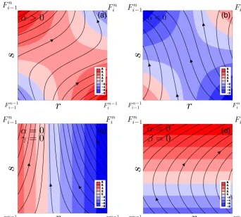
example of trajectories in this case is illustrated in Fig. 2a, with given values ofFin−−11,Fin−1,FinandFin−1. We see here
thatα >0 occurs when the flow changes from divergence in
theidirection at time stepn−1 to convergence at time step
Interpolated velocities
F(t)
∆ti
GCM velocities
∆tG t
n n+1
n-1 m
Figure 1.Schematic illustration of how the transport fieldsF (t )are updated and interpolated in time between the stored GCM data, which
are read in at the timetnand are separated in time by the time interval1tG(in red). The fields are then linearly interpolated at the points in blue with intermediate time steps. The number of intermediate time steps between two GCM velocities is in this exampleIS=1tG/1ti=4.
2.4.2 The caseα <0
When α <0, ξ becomes imaginary. By defining ζ≡iξ=
(β+αs)/
√
−2α, Eq. (31) can be re-expressed as
r(s)=r0+γ
α
eζ2−ζ02−γ
α−
βγ−αδ α
r π
−2αe
ζ2[erf(ζ )−erf(ζ
0)], (33)
where the error function erf(ζ )=(2/√(π )R0ζe−x2dx. An
ex-ample of trajectories for this case is illustrated in Fig. 2b. We see here thatα <0 occurs when the flow changes from
con-vergence in theidirection at time stepn−1 to divergence at time stepn.
2.4.3 The caseα=0
The solution of Eq. (26) whenα=0 is
r(s)=
r0+ δ
β
e−β(s−s0)−δ
β+ γ β2 h
1−βs+(βs0−1)e−β(s−s0)i. (34)
This case would normally not occur in a realistic GCM integration since it would correspond to a field constant in time or space, whereFin−Fin−1=Fin−1+Fin−−11. Note that if
the fields are in steady state, Eq. (34) is reduced to become identical to the stationary solution of Eq. (18). An example of trajectories in this stationary case is illustrated in Fig. 2c.
If insteadα=0 since the fields are constant in space, i.e. the transport across the grid cell is constant (Fi =Fi−1), then we also haveβ=0, which leads to a simplification of Eq. (26):
dr
ds+γ s+δ=0, (35)
with the solution
r(s)=r0−γ 2
s2−s02−δ (s−s0) . (36)
An example of trajectories in this case with constant fields in space is illustrated in Fig. 2d.
2.5 The transit time
A major difference between the time-dependent and the stepwise-stationary schemes is that in the time-dependent scheme, the transit timess1−s0cannot in general be obtained
explicitly with the time-dependent scheme in contrast to the stepwise-stationary analytical solution of Eq. (18). Using the solutions given by Eqs. (31)–(34), the relevant roots1of
r(s1)−r1=0 (37)
has to be computed numerically for each direction. We will now describe how the rootss1and the corresponding exiting
grid facer1can be determined. The displacement of the
tra-jectory inside the grid box under consideration then proceeds as previously discussed for stationary velocity fields.
We now determine the rootss1of Eq. (37) and the
cor-respondingr1 needed to calculate trajectories inside a grid
box. In what follows,sn−16s0< snand the relevant rootss1
are to be in the interval ofs0< s16sn. We also focus on the
casesα >0 andα <0, since the forthcoming considerations
can easily be adapted for the case ofα=0. For numerical purposes, we use
βγ−αδ
α =
FinFin−−11−Fin−1Fin−1
Fin−Fin−1−Fin−1+Fin−−11, (38) γ
α =
Fin−1−Fin−−11 Fin−Fin−1−Fin−1+Fin−−11
−ri−1, (39)
ξ =F
n−1 i−1 −F
n−1
i +α(s−sn −1) √
2α , (40)
ζ =F
n−1 i−1 −F
n−1
i +α(s−sn −1) √
−2α . (41)
As above,s is the scaled time. The coefficient in Eq. (38)
appearing in Eqs. (31) and (33) is exactly zero when either theri−1or ri grid face represents a solid boundary, so that transportFi or Fi−1 is zero for alln, respectively. In these instances, the opposite grid face fixesr1, and the roots1> s0
can be computed analytically. If there is no solution, we take
s1=sn. When all three transit times equalsn, the trajectory
(a)
(d) (c)
(b)
Figure 2.Examples of how trajectories calculated with the time-dependent scheme evolve as a function of the transportF in the space
intervalri−1< r < riand in the time intervalsn−1< s < sn, which hence corresponds to an interval between two GCM outputs (1tG) and
of a grid box (1x,1yor1z). The colour shows the transport valuesFobtained by the bilinear interpolation between the four corners (Fin−−11, Fin−1,FinandFin−1).(a)α >0 with two corners of transport in the negative direction(F <0), which correspond to westward, southward or downward directions, and one corner flowing in the opposite direction.(b)α <0.(c)α=0 andγ=0 correspond to the stationary fields, which results in anFfield that only changes in the(r)direction.(d)α=0 andβ=0 correspond to the constant fields in space but which vary in time. Note that theF=0 line between the red and blue colours corresponds to static flow, which results in “vertical” trajectories in the figures.
The roots of Eq. (37) have to be computed numerically if
(βγ−αδ)/α6=0. This is also true for locating the extrema of the solutions given by Eqs. (31) and (33). Alternatively, one can consider the case F (r, s)=0 using Eq. (24) to analyse where possible extrema are located. It follows that in thes−r
plane, the extrema lie on a hyperbola of the formr=(as+
b)/(c+ds). Obviously, only the parts defined bysn−1≤s≤
snandri−1≤r≤ri are relevant. Depending on which parts of the hyperbola, if any, lie in this “box” and satisfy the initial condition r(s0)=r0, the trajectory r(s)exhibits no, one or,
at most, two extrema. In the latter case, the trajectory will not cross either the grid face atri−1or the one atri (see Fig. 2
for an example). Hence, the trajectoriesr(s)determining the
transit times1−s0will have at most one extremum; i.e. there
is at most one change of sign in the local transportF.
An efficient way of proceeding is as follows: first, consider the grid face atri. For a trajectory to reach this grid face, the
local transport must be nonnegative, which depends on the
signs of the transportFin−1andFin. Four distinct
configura-tions may arise between the model outputs (sn−1< s < sn),
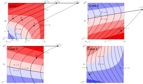
where the calculation of the trajectory takes place: 1. F (ri, s) >0 forsn−1< s < sn.
2. The sign ofF (ri, s)changes from positive to negative
ats=s∗, wheresn−1< s∗< sn.
3. The sign ofF (ri, s)changes from negative to positive
ats=s#, wheresn−1< s#< sn.
4. F (ri, s) <0 forsn−1< s < sn.
These four cases are illustrated by the four panels of Fig. 3. For case 1, we evaluater(sn)using the appropriate
ana-lytical solution. If, in addition,r(sn)≥ri, then the trajectory
has crossed the grid-box facer=ri ats1≤sn as shown by
the trajectories A, B and C in Fig. 3. If the initial transport
Case 1 Case 2
Case 3 Case 4
Figure 3.The four different cases of how trajectories might reach the grid face atr=ri. Note that the trajectories for case 4 can not reach
r=ri. The background colours are the same as in Fig. 2 withF >0 in red andF <0 in blue. The dashed trajectories outside the grid box
denote the necessary computed fictive paths for estimating whens=s1and if the trajectories reachr1(s1)=ri.
grid face at an earlier time, as illustrated by trajectory C in Fig. 3. This is only possible if case 3 applies for the grid face atri−1ands#> s0, in which case it is determined whether r(s#)≤ri−1. If this is not the case, there is a solution to r(s1)−r1=0 forr1=riands0< s1≤sn. Subsequently, this
root can be calculated numerically using a root-solving algo-rithm (Press et al., 2007). But ifr(sn) < ri or, if applicable, r(s#)≤ri−1, we proceed by considering the other grid faces. The arguments for the grid face at ri−1 are similar to those relating tori.
If case 2 applies and s0< s∗, we add here to the
consid-erations given in case 1 usings∗ instead ofsn. If there is a
root forr1=ri, thens0< s1≤s∗. This root is illustrated by
trajectoryDin Fig. 3 with(r1, s1)=(ri, s1D).
For case 3, we follow the procedure given by case 1. If there is a root forr1=ri, thens#< s1≤sn. This root is
il-lustrated by trajectoryEin Fig. 3 with(r1, s1)=(ri, s1E).
For case 4, no solution of Eq. (37) is possible forr1=ri,
since all trajectories exit through the grid face located atri−1, as illustrated by trajectoryGin Fig. 3, or will not reach any
grid face during the time interval sn−1< s < sn. We must
then instead search for an exit through another of the six grid faces.
All these considerations are applied to each of the three spatial directions in order to determine through which of the
six grid faces the trajectory will exit and at which position on the corresponding grid face.
Since the trajectories are unique solutions to Eq. (26) and the continuity equation is respected, the TRACMASS trajec-tories will therefore never hit any solid boundary, such as the coast or the sea floor, unless the sedimentation option is acti-vated, where an extra velocity is imposed, a feature that was introduced in TRACMASS by Corell and Döös (2013).
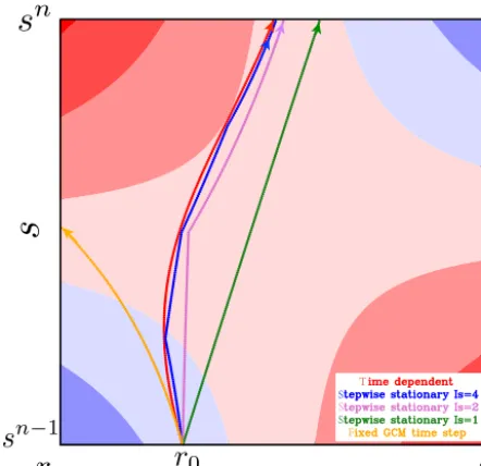
An example of the evolution of trajectories calculated with the three different schemes within a time–space cell forα >0 is shown in Fig. 4. The trajectories computed with
the stepwise-stationary scheme approach the trajectory com-puted with the time-dependent scheme with increasing num-ber of intermediate time steps (IS). The fixed GCM time step
trajectory can, however, not follow the time-dependent one since it does not update the velocities between the GCM out-puts and consequently deviates immediately as it leaves the initial point(r0, sn−1).
3 Tests with different velocity fields
The results obtained from the stepwise-stationary scheme are now compared with those from the time-dependent trajectory schemes using two different sets of velocity fields. The first uses a high-resolution OGCM withz-star coordinates. The
T S S S F
Figure 4.Example of how the trajectories differ when computed
with the fixed GCM time step method in orange, the stepwise-stationary method in blue, purple and green as well as the time-dependent method in red. They all start at the same timesn−1and in the same positionr0but exit the grid at different locations and times. Note that the stepwise-stationary method needs at least four intermediate time steps (IS) to be close to time-dependent trajec-tory. The background colours are the same as in Fig. 2 withF >0 in red andF <0 in blue.
with hybrid pressure coordinates. For the stepwise-stationary scheme, five different settings ofIS, i.e. the number of
inter-mediate steps, are tested. The fixed GCM time step is also tested for comparison, although it is not a standard feature of TRACMASS.
3.1 Ocean trajectories with a high-resolution OGCM Oceanic velocity fields for this case were obtained from a simulation with version 3.6 of the NEMO ocean model (Madec, 2016) in a global ORCA12 configuration. The hor-izontal resolution of the ORCA12 grid is approximately 1/12◦, corresponding to 1x≈6 km at 50◦ latitude. Model fields were available as 5-day averages every 5 days. The configuration uses 75z∗ vertical levels with partial bottom
cells, where 1zranges from ∼1 m at the surface to 250 m in the deepest parts of the ocean. Thez∗coordinate approach
permits large-amplitude free-surface variations relative to the vertical resolution (Adcroft and Campin, 2004). In thez∗
for-mulation, the variation of the column thickness due to sea-surface undulations is not concentrated to the sea-surface level, as in thez-coordinate formulation, but is equally distributed
over the full water column. Thus, the vertical levels naturally follow the sea-surface variations, which also implies that they are time dependent, and we therefore have used Eq. (12) to calculate the vertical transport in TRACMASS with a
time-dependent1znin the equation. The model was forced
with 6-hourly atmospheric fields from what is known as the Drakkar forcing set version 4 (DFS4) (Brodeau et al., 2010). Subgrid processes were represented using 125 m2s−1 Lapla-cian isoneutral tracer diffusion and−1.25×10¹⁰m4s−1 bi-Laplacian viscosity.
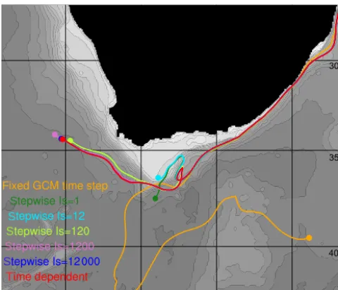
TRACMASS has been applied to this specific model inte-gration already by Nilsson et al. (2013), where it was com-pared with surface drifters in the Agulhas region. This is also the region where we are going to test TRACMASS because of its complex time-dependent dynamics with travelling ed-dies, known as “Agulhas rings”, which “leak” Indian Ocean water into the Atlantic Ocean as part of the conveyor belt. A total of 2193 trajectories were started, evenly spread over four horizontal grid boxes at all depths in the Indian Ocean and followed for 50 days as shown in Figs. 5 and 6.
3.2 Atmospheric trajectories with an AGCM
In order to test the trajectory schemes in the atmosphere, we have used the ERA-Interim reanalysis (Dee et al., 2011) from the European Centre for Medium-Range Weather Fore-casts (ECMWF) simulated with the IFS (Integrated Forecast-ing System) model. In this ERA-Interim data set, the verti-cal coordinate is a terrain-following hybrid coordinate (Sim-mons and Burridge, 1981), where the pressure at the lower interface of levelk is given bypk=Ak+Bkps, where ps
is the surface pressure and Ak and Bk are parameters at
the level k∈ [0,60], with p60=ps andp0=0. As in the NEMO ocean model, the grid cell thickness varies in time, and we calculate vertical mass flux from the continuity equa-tion (Eq. 15). The ERA-Interim data used here had a hori-zontal resolution of 1.25◦ and is available 6-hourly (1tG).
Trajectories are shown in Fig. 7. They were initiated every 6 h from a grid cell air column over the Eyjafjallajökull vol-cano eruption during 14–18 March 2010. The trajectories were evenly distributed horizontally and started in exactly same positions for the tests with different time steps using the stepwise-stationary scheme and time-dependent case. 3.3 Lagrangian statistics
inter-6 6 6
( ( (
( (
Figure 5.Agulhas trajectories started evenly distributed in a square of four grid cells and followed for 50 days. Colouring is used to separate
the trajectories from each other.
Table 1.The table shows the average distance between the time-dependent integrated trajectories and the stepwise-stationary integrated ones
at the end of simulations, which is 50 days for the OGCM and 10 days for the AGCM.ISis the number of intermediate time steps between two GCM outputs. The “maximum time step” stands for the intermediate time step lengths(1ti), which are used in the different trajectory integrations. The last column is the computational time normalised with regard to the time-dependent case, where theoretical velocity fields are used to compute trajectories, i.e. with no data reading or writing.
Distance to time dependent TL Maximum time step Normalised
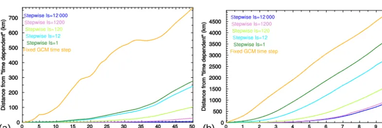
OGCM AGCM AGCM OGCM OGCM computational
IS (km) (km) (days) 1ti 1ti Time
Fixed 769 4992 3.44 ≡5 d ≡6 h 0.830
1 276 3835 3.88 5 d 6 h 0.830
12 242 2971 3.86 10 h 30 min 2.110
120 103 1752 3.86 1 h 3 min 14.03
1200 28 1079 3.87 6 min 18 s 132.0
12 000 6 1002 3.87 36 s 2 s 1191
Time dependent 0 0 3.87 5 d 6 h 1.000
mediate time steps are used, shows the greatest distance to the time-dependent case.
Standard Lagrangian statistics have also been computed for the ocean trajectories (Fig. 9), with the definitions given in the Appendix. The “relative” and “absolute dispersion” as well as the “mean displacement” of the trajectory cluster show how the cluster will disperse and move in time. They reveal a similar pattern, where only the fixed GCM time step case differs from the others. The fixed GCM time step differs
already after 3 to 4 days, which should be related to the fact that the GCM velocities are updated every 5 days (=1tG) in
this OGCM case.
40° S 35° S 30° S
20° E 25°E 30°E
15° E
F
S S
S
S
S
T
Figure 6.Example of ocean trajectory paths due to different
tra-jectory schemes and number of intermediate time steps. The time-dependent method results are in red as well as those obtained with the stepwise-stationary method withIS=1,12,120,1200 and 12 000 as well as fixed GCM time steps. Note that these homolo-gous trajectories were selected to illustrate that stepwise-stationary trajectories are closer to time-dependent trajectories when the num-ber of intermediate time steps(IS)is increased.
memory of the trajectories, reflects the same feature with a Lagrangian timescale of approximately 3.9 days for the time step and the time-dependent cases but a slightly shorter timescale of 3.4 days for the fixed GCM time step case. The Lagrangian timescale based on observations with surface drifters is clearly shorter than this both for the global ocean (Döös et al., 2011) and in the Agulhas region (Nilsson et al., 2013). This relatively shorter Lagrangian timescale (hence closer to observations for the fixed GCM time step) is simply due to the abrupt changes in the velocity fields every time these are updated. A realistic shortening of the Lagrangian timescale can only be obtained by incorporating finer scales by increasing the GCM resolution or adding subgrid param-eterisations to the trajectories.
The power spectra computed from the Lagrangian veloci-ties show that the fixed GCM time step was more energetic than the other schemes, which all yielded nearly identical re-sults. This is the case for all frequencies. There is also a weak maximum at four cycles per day (6 h), which remains unex-plained, although it may be related to the fact that the OGCM uses 6-hourly atmospheric forcing.
3.4 Lagrangian stream function and residence time The mass conservation properties of the used trajectory schemes make it possible to calculate mass transports be-tween different sections in the model domain (Döös, 1995). The approach is that one can associate each trajectory
par-ticle with a mass or volume transport. This requires that enough trajectories are computed to fill the model grid in space and time with a sufficient number of trajectories. La-grangian stream functions can be calculated by summing over trajectories representing a desired path (Blanke et al., 1999; Döös et al., 2008; Kjellsson and Döös, 2012b). The difference between the Lagrangian and the more common Eulerian stream functions is that with the Lagrangian one can isolate a particular path between a starting and an ending sec-tion in the ocean or the atmosphere.
The influence of the different trajectory schemes on the inter-ocean exchange of water masses, which takes place in the Agulhas region, has been evaluated by calculating La-grangian stream functions. Figure 10 shows the LaLa-grangian barotropic stream function computed from trajectories using the time-dependent scheme and the fixed GCM time step scheme. Lagrangian decomposition has been used to com-pute two separate stream functions for each scheme, one from trajectories entering the Atlantic and one from those re-turning back into the Indian Ocean via the Agulhas retroflec-tion region. The time-dependent scheme favours slightly (one additional stream line) the entering into the Atlantic com-pared to the fixed GCM time step scheme. This is also clearly visible when computing the residence time; i.e. the time tra-jectories stay within the Agulhas region as shown in the lower righthand panel of Fig. 9. The first particles start to exit the Agulhas region, as defined by the map in Fig. 10, after 50 days. The number of trajectory particles then decays exponentially with ane-folding time of about 210 days. This
is rather similar for all trajectory-scheme integrations. There is, however a clear difference in the results where the trajec-tories exit. The fixed GCM time step scheme results in 38 % flowing into the Atlantic and 59 % into the Indian Ocean after 800 days. All the other trajectory integrations yield very sim-ilar results but with 46 % flowing into the Atlantic and 52 % into the Indian Ocean. This suggests that the fixed GCM time step scheme does not capture the same behaviour as the other schemes.
We have repeated the above ocean-trajectory experiment by releasing the particles in other time periods and increasing the ensemble size. The results only changed marginally. 3.5 Computational speed
1744 K. Döös et al.: Evaluation of oceanic and atmospheric trajectory schemes
S
S
S
S
S
T F
S
Figure 7.Example of atmospheric trajectory paths starting form the Eyjafjallajökull volcano during its eruption calculated with different
trajectory schemes and number of intermediate time steps. The same colour coding of the trajectories as in Fig. 6 is used. Note that the red time-dependent and the blue stepwise schemes withIS=12 000 trajectories are nearly identical.
Distance from "time dependent" (km)
Time (days) 0
100 200 300 400 500 600 700
0 5 10 15 20 25 30 35 40 45 50
Distance from "time dependent" (km)
Time (days) 0
500 1000 1500 2000 2500 3000 3500 4000 4500
0 1 2 3 4 5 6 7 8 9 10
Figure 8.Average distance between the "time-dependent" trajectories and the "stepwise-stationary" ones for the different time-steps with
IS= 1,12,120,1200and12000as well as "fixed GCM time steps". The left panel represents the ocean Agulhas trajectories and the right
panel the atmospheric ERA-Interim ones. Note that the more intermediate steps used by the "stepwise-stationary" scheme the closer results to the "time-dependent" scheme.
26
S
S S
S
F
S
S
S S
S
F
S
(a) (b)
Figure 8.Average distance between the time-dependent trajectories and the stepwise-stationary ones for the different time steps withIS=
1,12,120,1200 and 12 000 as well as fixed GCM time steps. The left panel represents the ocean Agulhas trajectories and the right panel the atmospheric ERA-Interim ones. Note that the more intermediate steps used by the stepwise-stationary scheme the closer results to the time-dependent scheme.
The stepwise-stationary scheme was only as computationally fast as the time-dependent scheme when no extra intermedi-ate time steps were taken between two readings of the ve-locity fields (IS=1) or when using fixed GCM time steps. When the number of intermediate time steps was increased to 12 000, the stepwise-stationary scheme was more than 1000 times slower. The total of 12 000 intermediate steps was also approximately the number of intermediate time steps re-quired in order to obtain as accurate results as those obtained from the time-dependent scheme.
4 Discussion and Conclusions
The two trajectory schemes available in TRACMASS have here been intercompared by calculating Lagrangian statis-tics, transports and the distances between the trajectories. This has been done for both oceanic and atmospheric ap-plications. The stepwise-stationary scheme assumed that the velocity fields were stationary for the duration of a user-defined intermediate time step between model output fields. These velocities are, however, updated with a linear interpo-lation in time when crossing a model grid face. The
time-dependent scheme does not assume that the velocity is in steady state during any time interval since it solves the differ-ential equations of the trajectory path not only in space but also in time. This continuous evolution of the time-dependent scheme makes it more accurate than the stepwise-stationary scheme without any significant increase in computational ex-pense.
In addition to these two TRACMASS schemes, we have tested a fixed GCM time step scheme, which is in fact a spe-cial case of the stepwise-stationary scheme but with velocity fields always remaining in steady state until a new GCM data set is reloaded in order to mimic the Ariane trajectory model (Blanke and Raynaud, 1997). A consequence of only updat-ing the fields at the GCM output times is that the velocities are assumed to be in steady state for long periods and then changed abruptly with a discontinuity.
aver-Relative dispersion (km) Time (days) 0 50 100 150 200 250 300 350 400 450 500 550
0 5 10 15 20 25 30 35 40 45 50
Absolute dispersion (km)
Time (days) 0 100 200 300 400 500 600 700 800 900 1000
0 5 10 15 20 25 30 35 40 45 50
Mean displacement (km)
Time (days) 0 100 200 300 400 500 600 700 800 900
0 5 10 15 20 25 30 35 40 45 50
Autocorrelation Time (days) 0 .1 .2 .3 .4 .5 .6 .7 .8 .9 1.0 -.1 -.2 -.3
0 5 10 15 20 25 30 35 40 45 50
Power spectra (m2/(c.p.d.s2))
Cycles (1/day)
10-3 10-2 10-1
10-1 100
Trajectories (%)
Residence time (days)
0 10 20 30 40 50 60 70 80 90 100
0 100 200 300 400 500 600 700 800
Figure 9. Lagrangian statistics of the ocean Agulhas trajectories. The relative dispersion (top left), the absolute dispersion (top right),
the mean displacement travelled by the trajectory cluster (middle left), the average Lagrangian velocity autocorrelation of the trajectories (middle right). The average power spectra of the Lagrangian velocities (lower left). The residence time evolution of the trajectory particles in the Agulhas region. Note that all statistics show very similar results, where only those based on the "fixed GCM time step" (orange curves) differ from the rest.
27 S S S S F S T S S S S F S T S S S S F S T S S S S F S T S S S S F S T S S S S F S T T
(a)
(b)
(c)
(d)
(e)
(f)
Figure 9.Lagrangian statistics of the ocean Agulhas trajectories. The relative dispersion(a), the absolute dispersion(b), the mean
displace-ment travelled by the trajectory cluster(c), the average Lagrangian velocity autocorrelation of the trajectories(d)and the average power spectra of the Lagrangian velocities(e)and the residence time evolution of the trajectory particles in the Agulhas region(f)are shown. Note that all statistics show very similar results, where only those based on the fixed GCM time step (orange curves) differ from the rest.
age distance as a function of time between the trajectories obtained from the different schemes is shown in Fig. 8, and their end position distances are shown in Table 1.
The study has shown that the TRACMASS time-dependent scheme is likely to be more accurate as well as faster than the stepwise-stationary scheme with inter-mediate steps. It remains to be shown how the trajectory schemes used in the present study compare to other trajec-tory schemes, e.g. Runge–Kutta, which could be used where mass conservation is not important.
The stepwise-stationary scheme needed up to 12 000 in-termediate time steps to give as accurate trajectory paths as the time-dependent scheme, which is more than a thousand times as computationally expensive when reading and
Figure 10.The Lagrangian decomposed barotropic stream function based on the particles released as previously but followed until they left the Agulhas region into the Atlantic(a, c)or the Indian Ocean(b, d). The top panels show the time-dependent scheme and the lower panels show the fixed GCM time step scheme. Note that there is more water (one stream line extra) flowing into the Atlantic with the time-dependent scheme than with the fixed GCM time step scheme, which instead favours relatively the flow into the Indian Ocean. Stream line intervals of 8 Sv(106m3s−1) are shown.
could be to calculate trajectories first using fields stored at each GCM time step and then using fields stored at longer time intervals. In the first case, trajectories would be very accurate and could represent a “truth”, and the second case could be used to evaluate which scheme is the closest to the truth.
The Lagrangian statistics, such as relative and absolute dispersion as well as Lagrangian velocity autocorrelation functions and power spectra, showed almost identical results for the time-dependent and the stepwise-stationary schemes. The fixed GCM time step showed, however, some differ-ences from the other two schemes. For example, the disper-sion after 3–4 days was slightly larger for using a fixed GCM time step, which might be explained by an abrupt change ev-ery time the GCM velocities are updated compared to the smoother transition of the two other schemes. The results show that the fixed GCM time step method does not cap-ture the same behaviour of trajectories as the other schemes. The Lagrangian statistics are also clearly affected by the model resolution and the time sampling of the GCM fields (Döös et al., 2011; Kjellsson and Döös, 2012a; Kjellsson et al., 2013; Nilsson et al., 2013). Future improvements to
the TRACMASS model will involve improvements of the subgrid turbulence parameterisations, which could give more realistic dispersion properties.
and stepwise-stationary schemes than by the fixed GCM time step scheme.
The TRACMASS trajectory code with corresponding schemes has been improved and has become more accurate and user friendly over the years. An outcome of the present study is that we strongly recommend the use of the time-dependent scheme based on de Vries and Döös (2001) in favour of the stepwise-stationary scheme. We would also like to dissuade the use of the more primitive fixed GCM time step scheme, which is used in other trajectory codes, since the velocity fields remain stationary for longer periods, creating abrupt discontinuities in the velocity fields and yielding in-accurate solutions. We have only tested one OGCM and one AGCM simulation here, but we speculate that at coarser res-olution in both space and time, the differences obtained with the two schemes would increase. However, in non-eddying simulations (e.g. 1◦ocean models) this may not be true due to the low variability of the flow.
The TRACMASS strict requirement of mass conservation makes it, however, necessary to have complete velocity fields on the original GCM grid in order to use mass or volume transports in and out of each model grid box. This require-ment of mass conservation will always be somewhat more demanding than for other trajectory codes, since it requires a total understanding of the various GCM coordinate sys-tems as well as the incorporation of them in the TRACMASS framework. This state of affairs is in marked contrast to what holds true for various trajectory codes that only require ve-locity fields with no mass conservation.
Appendix A: Lagrangian statistics definitions
The Lagrangian statistics used in the present work (shown in Figs. 8 and 9) are here defined. See, e.g. LaCasce (2008) for a detailed derivation.
The average distance between the different trajectory cal-culations, as presented in Fig. 8, is defined as
DB2(t )≡ 1
M−1
N X
m=1 2 X
i=1
xi,m(t )− ˆxi,m(t )2. (A1)
It is hence the distance between the two trajectories,xi,m(t )
andxˆi,m(t ), wheret is the time,M the total number of
tra-jectories of the cluster andithe spatial coordinate index (i.e.
the zonal, meridional or vertical position of themth
trajec-tory xi,m(t )). The two trajectories,xi,m(t )andxi,m(t )ˆ , will have the same initial position xi,m(t0)= ˆxi,m(t0) but will
then evolve differently since different trajectory schemes are used to compute their paths. In the present study, we only consider the horizontal dispersion. The vertical dispersion is, however, an important measure of the vertical mixing in the ocean but beyond the scope of the present study.
The mean position of the trajectory cluster is defined as
xi(t )≡
1
M M X
m=1
xi,m(t ). (A2)
The relative dispersion is defined as the mean square dis-placement of the trajectories relative to the time-evolving mean position:
DR2(t )≡ 1
M−1
M X
m=1 2 X
i=1
xi,m(t )−xi(t ) 2
. (A3)
The absolute dispersion is defined in the same way, but rela-tive to the initial position of the cluster:
DA2(t )≡ 1
M−1
M X
m=1 2 X
i=1
xi,m(t )−xi(t0) 2
, (A4)
wheret0is the initial time of the trajectory.
The mean displacement is defined as the displacement from the origin as a function of time:
DD(t )≡
1
M M X
m=1 v u u t 2 X
i=1
xi,m(t )−xi,m(t0)2. (A5)
The Lagrangian velocity is obtained by using a non-centred finite difference:
ui,m(tn)≡
dxi,m(tn)
dt ≈
xi,m(tn)−xi,m(tn−1)
tn−tn−1 , (A6) wherenis the time level. Similarly, the acceleration was
cal-culated by finite differencing of the velocity:
ai,m(tn)≡dui,m(t
n)
dt ≈
ui,m(tn)−ui,m(tn−1)
tn−tn−1 . (A7)
Note how velocity is not defined at the first position, and ac-celeration is not defined at the first velocity.
The Lagrangian velocity autocorrelation describes the cor-relation of the velocity at one time with that of previous times. The definition is
R(τ )= σ 2(τ )
σ2(τ=0)≈R(t
q)(σ (tq))2
(σ (t0))2, (A8)
whereσ2(τ )andσ2(τ=0)are the Lagrangian velocity
au-tocovariances for time lagτ and no lag, respectively.qis the
discrete time step andRq is the autocorrelation at time step q.σ2(τ )is defined as
σ2(τ )= lim
T→∞ 1 T T Z 0
u0(t+τ )·u0(t )dt≈(σ (tq))2
≡ 2 X
i=1 1
N−q−1
N−q−1 X
n=1
u0i(tn)u0i(tn+q), (A9)
whereu0i(tn)=ui(tn)−ui andui is a time average of the
segment. Note that the total velocity autocovariance is the sum of the zonal and meridional components,σ2=σi2=1+
σi2=2.
The Lagrangian timescale is defined as
TL= ∞ Z
0
R(τ )dτ. (A10)
Competing interests. The authors declare that they have no conflict of interest.
Acknowledgements. The authors wish to thank Peter Lundberg for constructive comments. This work has been financially supported by the Bolin Centre for Climate Research and by the Swedish Research Council (Grant 2015-04442). Joakim Kjellsson is supported by the UK Natural Environment Research Council grant NE/K012150/1: “Poles apart: why has Antarc-tic sea ice increased, and why can’t coupled climate models reproduce observations?”. The GCM integrations and the tra-jectory computations were performed using resources provided by the Swedish National Infrastructure for Computing (SNIC) at the National Supercomputer Centre at Linköping University (NSC).
Edited by: R. Marsh
Reviewed by: S. M. Griffies and two anonymous referees
References
Adcroft, A. and Campin, J.-M.: Rescaled height coordi-nates for accurate representation of free-surface flows in ocean circulation models, Ocean Model., 7, 269–284, doi:10.1016/j.ocemod.2003.09.003, 2004.
Blanke, B. and Raynaud, S.: Kinematics of the Pacific Equatorial Undercurrent: a Eulerian and Lagrangian approach from GCM results, J. Phys. Oceanogr., 27, 1038–1053, 1997.
Blanke, B., Arhan, M., Madec, G., and Roche, S.: Warm water paths in the equatorial Atlantic as diagnosed with a general circulation model, J. Phys. Oceanogr., 29, 2753–2768, 1999.
Brodeau, L., Barnier, B., Treguier, A.-M., Penduff, T., and Gulev, S.: An ERA40-based atmospheric forcing for global ocean circulation models, Ocean Model., 31, 88–104, doi:10.1016/j.ocemod.2009.10.005, 2010.
Butcher, J. C.: Numerical Methods for Ordinary Differential Equa-tions, John Wiley & Sons, Ltd, doi:10.1002/9781119121534, 2016.
Corell, H. and Döös, K.: Difference in Particle Transport Be-tween Two Coastal Areas in the Baltic Sea Investigated with High-Resolution Trajectory Modeling, AMBIO, 42, 455–463, doi:10.1007/s13280-013-0397-3, 2013.
Dee, D. P., Uppala, S. M., Simmons, A. J., Berrisford, P., Poli, P., Kobayashi, S., Andrae, U., Balmaseda, M. A., Balsamo, G., Bauer, P., and Bechtold, P.: The ERA-Interim reanalysis: config-uration and performance of the data assimilation system, Q. J. Roy. Meteor. Soc., 137, 553–597, doi:10.1002/qj.828, 2011. de Vries, P. and Döös, K.: Calculating Lagrangian trajectories
us-ing time-dependent velocity fields, J. Atmos. Ocean. Tech., 18, 1092–1101, 2001.
Döös, K.: Inter-ocean exchange of water masses, J. Geophys. Res., 100, 13499–13514, 1995.
Döös, K. and Engqvist, A.: Assessment of water exchange between a discharge region and the open sea–a comparison of different methodological concepts, Estuarine, Coast. Shelf Sci., 74, 709– 721, 2007.
Döös, K., Nycander, J., and Coward, A.: Lagrangian decompo-sition of the Deacon Cell., J. Geophys. Res., 113, C07028, doi:10.1029/2007JC004351, 2008.
Döös, K., Rupolo, V., and Brodeau, L.: Dispersion of surface drifters and model-simulated trajectories, Ocean Model., 39, 301–310, doi:10.1016/j.ocemod.2011.05.005, 2011.
Döös, K., Kjellsson, J., and Jönsson, B.: TRACMASS – A La-grangian Trajectory Model, Preventive Methods for Coastal Pollution: towards the Use of Ocean Dynamics for Pollution Control, chap. 7, Springer International Publishing, 225–249, doi:10.1007/978-3-319-00440-2_7, 2013.
Fabbroni, N.: Numerical simulations of passive tracers dispersion in the sea, Alma Mater Studiorum, Universita di Bologna, PhD Thesis, 164 pp., doi:10.6092/unibo/amsdottorato/1733, 2009. Jönsson, B., Döös, and Kjellsson, J.: TRACMASS: Lagrangian
tra-jectory code, doi:10.5281/zenodo.34157, 2015.
Kjellsson, J. and Döös, K.: Surface drifters and model trajectories in the Baltic Sea, Boreal Environ. Res., 17, 447–459, 2012a. Kjellsson, J. and Döös, K.: Lagrangian decomposition of the
Hadley and Ferrel cells, Geophys. Res. Lett., 39, L15807, doi:10.1029/2012GL052420, 2012b.
Kjellsson, J., Döös, K., and Soomere, T.: Evaluation and Tuning of Model Trajectories and Spreading Rates in the Baltic Sea Using Surface Drifter Observations, 251–281, Springer Inter-national Publishing, Heidelberg, doi:10.1007/978-3-319-00440-2_8, 2013.
LaCasce, J.: Statistics from Lagrangian observations, Prog. Oceanogr., 77, 1–29, doi:10.1016/j.pocean.2008.02.002, 2008. Madec, G.: NEMO ocean engine, Version 3.6., France, Institut
Pierre-Simon Laplace (IPSL), Note du Pole de Modélisation, 396 pp., 2016.
Marsh, R. and Megann, A. P.: Tracing water masses with particle trajectories in an isopycnic-coordinate model of the global ocean, Ocean Model., 4, 27–53, 2002.
Nilsson, J. A. U., Döös, K., Ruti, P. M., Artale, V., Coward, A., and Brodeau, L.: Observed and Modeled Global Ocean Tur-bulence Regimes as Deduced from Surface Trajectory Data, J. Phys. Oceanogr., 43, 2249–2269, doi:10.1175/JPO-D-12-0193.1, 2013.
Press, W. H., Teukolsky, S. A., Vetterling, W. T., and Flannery, B. P.: Numerical Recipes 3rd Edition: The Art of Scientific Comput-ing, Cambridge University Press, New York, NY, USA, 3rd Edn., 2007.
Simmons, A. J. and Burridge, D. M.: An Energy and Angular-Momentum Conserving Vertical Finite-Difference Scheme and Hybrid Vertical Coordinates, Mon. Weather Rev., 109, 758–766, 1981.