A joint global carbon inversion system using both CO 2and13 CO 2 atmospheric concentration data

www.geosci-model-dev.net/10/1131/2017/ doi:10.5194/gmd-10-1131-2017

© Author(s) 2017. CC Attribution 3.0 License.

A joint global carbon inversion system using both CO

2

and

13

CO

2

atmospheric concentration data

Jing M. Chen1,2, Gang Mo2, and Feng Deng2

1_{International Institute of Earth System Science, Nanjing University, 22 Hankou Road, Nanjing, Jiangsu, China} 2_{Department of Geography and Program in Planning, University of Toronto, Toronto, Ontario, Canada}

Correspondence to:Jing M. Chen ([email protected]) Received: 6 March 2016 – Discussion started: 17 May 2016

Revised: 15 February 2017 – Accepted: 17 February 2017 – Published: 16 March 2017

Abstract. Observations of 13CO2 at 73 sites compiled in

the GLOBALVIEW database are used for an additional con-straint in a global atmospheric inversion of the surface CO2

flux using CO2observations at 210 sites (62 collocated with

13_CO

2 sites) for the 2002–2004 period for 39 land regions

and 11 ocean regions. This constraint is implemented us-ing prior CO2fluxes estimated with a terrestrial ecosystem

model and an ocean model. These models simulate 13CO2

discrimination rates of terrestrial photosynthesis and ocean– atmosphere diffusion processes. In both models, the 13CO2

disequilibrium between fluxes to and from the atmosphere is considered due to the historical change in atmospheric13CO2

concentration. This joint inversion system using both13CO2

and CO2 observations is effectively a double deconvolution

system with consideration of the spatial variations of isotopic discrimination and disequilibrium. Compared to the CO2

-only inversion, this13CO2constraint on the inversion

consid-erably reduces the total land carbon sink from 3.40±0.84 to 2.53±0.93 Pg C year−1but increases the total oceanic car-bon sink from 1.48±0.40 to 2.36±0.49 Pg C year−1. This constraint also changes the spatial distribution of the car-bon sink. The largest sink increase occurs in the Amazon, while the largest source increases are in southern Africa, and Asia, where CO2 data are sparse. Through a case study, in

which the spatial distribution of the annual 13CO2

discrim-ination rate over land is ignored by treating it as a con-stant at the global average of −14.1 ‰, the spatial distri-bution of the inverted CO2 flux over land was found to be

significantly modified (up to 15 % for some regions). The uncertainties in our disequilibrium flux estimation are 8.0 and 12.7 Pg C year−1‰ for land and ocean, respectively. These uncertainties induced the unpredictability of 0.47 and

0.54 Pg C year−1 in the inverted CO2 fluxes for land and

ocean, respectively. Our joint inversion system is therefore useful for improving the partitioning between ocean and land sinks and the spatial distribution of the inverted carbon flux.

1 Introduction

Over the last few decades, much progress has been made in estimating the global carbon cycle using different methods (Houghton et al., 2007; Canadell et al., 2007; Le Quéré et al., 2013). In particular, atmospheric CO2 mole fractions

mea-sured near the surface have been used to infer the carbon flux over land and ocean surfaces through atmospheric inversion (Rödenbeck et al., 2003; Michalak et al., 2005; Peylin et al., 2005; Peters et al., 2007). However, the uncertainty in the inferred flux is still very large, mostly because of the insuf-ficient number of observation stations and the error in mod-elling the atmospheric transport of CO2from the surface to

the observation stations. To reduce this uncertainty, it would be useful to introduce constraints to the inversion using other gas species that are associated the CO2flux.

Measurements of the atmospheric concentration of the stable isotope 13CO2 at a number of stations across

the globe since 1994 have been compiled in a database (GLOBALVIEW-CO2C13, 2009), and the number of ex-tended13CO2 records from January 1994 to January 2009

increased to 76 by 2009. The mole fraction of 13CO2 to

CO2 in the atmosphere is about 1.1 %, and the CO2

ex-change between the surface and the atmosphere generally induces concurrent13CO2 exchange. However, the

dif-ferent locations and difdif-ferent times due to difdif-ferent mecha-nisms that discriminate against heavier13CO2molecules in

the exchange processes, and therefore the13CO2

concentra-tion measured in the atmosphere contains addiconcentra-tional infor-mation for the CO2flux. This information is useful for

dif-ferentiating between terrestrial and oceanic CO2exchanges

with the atmosphere because the terrestrial CO2flux

experi-ences much greater discrimination against13CO2than does

the oceanic CO2flux (Tans et al., 1990; Ciais et al., 1995a;

Francey et al., 1995). Observed 13CO2 mole fractions can

also provide independent information on the net CO2

ex-change over land and ocean because the net carbon flux to the surface discriminates against heavier13CO2(Fung et al.,

1997; Randerson et al., 2002; Suits et al., 2005). The13CO2

observations over the globe, albeit with a limited number of stations, could therefore be used to assist in quantifying the global carbon cycle.

In previous studies (Siegenthaler and Oeschger, 1987; Keeling et al., 1989a; Francey et al., 1995; Randerson et al., 2002), atmospheric13CO2observations have been used

to separate ocean and land CO2fluxes through the use of a

technique dubbed “double deconvolution”, by which the CO2

fluxes of land and ocean are separated (deconvolved) based on different discrimination rates against13CO2in the

atmo-spheric CO2 exchange with land and ocean surfaces. This

double deconvolution often assumes that the discrimination rates over land and ocean are spatially uniform, although they can be temporally variable. Through forward atmospheric transport modelling, the ocean and land CO2 fluxes were

also separated based on the spatial gradients of the measured

13_CO

2/CO2ratio either globally (Keeling et al., 1989b) or

by latitudinal bands (Ciais et al., 1995a). The same 13CO2

data have also been used in inverse modelling of the surface CO2flux (Enting et al., 1995; Rayner et al., 1999, 2008).

Ent-ing et al. (1995) pioneered a methodology for invertEnt-ing an-nual mean ocean and land CO2fluxes from both atmospheric

CO2and13CO2concentration data for 12 ocean regions and

8 land ecosystems for the 1986–1987 and 1989–1990 peri-ods. Rayner et al. (1999) developed a different methodology to invert monthly CO2 fluxes for 12 ocean and 14 land

re-gions for the period from 1980 to 1995 from CO2

observa-tions at 12 staobserva-tions and13CO2and O2/N2observations at 1

station. Rayner et al. (2008) refined their methodology and applied it to the period from 1992 to 2005 using CO2at 67

sites and13CO2at 10 sites. These studies showed the

useful-ness of the additional information from13CO2observations

in improving the inversion of annual mean and seasonality of the CO2flux over land and ocean. In these inversion studies,

the discrimination rate for land is either assumed to be a con-stant (Enting et al., 1995; Rayner et al., 1999) or allowed to vary with the areal fraction of C4 plant in a region (Rayner et al., 2008). These inversions based on the Bayesian principle were also constrained with only simple prior estimates of the terrestrial and oceanic CO2and13CO2fluxes. Since the data

density (the numbers of CO2and13CO2 observation sites)

is low, the assumed discrimination constants and these prior estimates would have considerable influence on the inverted results, as this is clearly demonstrated in Enting et al. (1995). Atmospheric CO2 observations have been extensively

used to estimate the carbon flux over ocean and land through inverse modelling using Bayesian synthesis (Gurney et al., 2002; Rödenbeck et al., 2003; Baker et al., 2006; Peylin et al., 2005) or data assimilation techniques (Peters et al., 2007; Zhang et al., 2014). Atmospheric inversion studies (Gurney et al., 2003; Jacobson et al., 2007) often produced ocean sinks considerably smaller than those estimated based on ob-served gradients in dissolved inorganic carbon (DIC) in in-terior ocean using ocean circulation models (Steinkamp and Gruber, 2013). Recent estimates for the ocean sink for an-thropogenic CO2 in the 2000s were based on DIC ranges

from 1.6 to 2.6 Pg C year−1(Park et al., 2010; Wanninkhof et al., 2013; Landschützer et al., 2014; Majkut et al., 2014; DeVries, 2014; Rödenbeck et al., 2014) with an uncertainty of about 0.6 Pg C year−1, while atmospheric inversion re-sults are not yet reliable enough to be included in a global ocean sink synthesis (Le Quéré et al., 2013). The partition between ocean and land fluxes using atmospheric inversion techniques is sensitive to errors in atmospheric transport modelling (Patra et al., 2005; Baker et al., 2006; Stephens et al., 2007) and prior fluxes for land and ocean used to con-strain the inversion (Zhang et al., 2014; Chen et al., 2015). It would therefore be highly desirable to use13CO2

observa-tions to constrain this partition in the inversion process. An accurate partition between ocean and land sinks is important in global carbon cycle research because (1) land sinks are still more reliably estimated as the residual of the global car-bon budget than those from land-based data (Le Quéré et al., 2013) and (2) ocean sink estimates based on DIC in ocean water also suffer from considerable errors due to insufficient DIC observations and ocean circulation modelling (DeVries, 2014).

The overall goal of this study is to explore the information content of13CO2measurements for global CO2flux

estima-tion through developing a Bayesian synthesis inversion sys-tem that uses both CO2 and13CO2observations. This

sys-tem is effectively a new double deconvolution syssys-tem with the capacity of considering the spatial variations of the prior carbon flux and all major isotopic parameters including pho-tosynthetic discrimination, respiratory signature and disequi-librium rate. In this study, this new system is used to achieve the following objectives: (1) to partition between ocean and land sinks with consideration of the spatial distributions of

13_CO

2isotopic parameters over ocean and land, (2) to

eval-uate the importance of considering the spatial distributions of the13CO2 discrimination rate over land in the inversion

of the CO2flux and (3) to assess the impacts of the errors

Figure 1.A global nested inversion system with a focus in North America, in which oceans are divided into 11 regions and land areas are divided into 9 large and 30 small regions outside and within North America, respectively. Also shown are CO2and13CO2observation

stations included in the GLOBALVIEW database and used in this study; 10 of the stations are marked with their names because they are selected to compare prior and posterior concentrations in Fig. 11.

spatial distributions of the13CO2discrimination and

disequi-librium rates over land for use in a global Bayesian synthesis inversion with 13CO2constraint. BEPS is also used to

pro-duce CO2prior fluxes globally to regularize the inversion.

2 Methodology

2.1 The inversion method

2.1.1 Inversion system

The nested inversion system with a focus on North Amer-ica developed by Deng et al. (2007) is adopted in this study. In this system, two of the Transcom regions (Gurney et al., 2002) in North America are divided into 30 regions ac-cording to ecosystem types and administrative boundaries (Fig. 1), in order to reduce spatial aggregation errors in the inversion over North America and to investigate the in-verted spatial distribution of the carbon flux against ecosys-tem model results. This nested region serves the purpose of evaluating the influence of the spatial distribution of iso-topic discrimination on the inverted carbon flux at a relatively high resolution. Also shown in Fig. 1 are the spatial distribu-tions of 210 CO2and 7313CO2observation sites selected in

this study from the NOAA GLOBALVIEW database. Most

13_CO

2sites (except 11) are collocated with CO2sites. 2.1.2 Synthesis Bayesian inversion with CO2

observations

To estimate the CO2flux (f), we represent the relationship

between CO2measurements and the flux from the surface by

a linear model:

c=Gf+Ac0+ε, (1)

wherecm×1 is a given vector ofm CO2 concentration

ob-servations over space and time (mequals number of stations times number of months, and for CO2-only inversion; it is

12 600, i.e. 210 stations×60 months, 2000–2004); εm×1is

a random error vector with a zero mean and a covariance matrix cov(ε)=Rm×m;Gm×(n−1)is a matrix representing a transport (observation) operator, wheren−1 is the number of fluxes to be determined (equals 3000, i.e. 50 regions×60 months, 2000–2004); Am×1 is a unity vector (filled with

1) representing the assumed initial well-mixed atmospheric CO2concentrations (c0)before the first month; andf(n−1)×1

is an unknown vector of monthly carbon fluxes of the 50 re-gions.

Combining matrixesGandAasMm×n=(G,A)and vec-torsf andc0assn×1=(fT,c0)T, Eq. (1) can be expressed

as

c=Ms+ε. (2)

function: J =1

2(Ms−c)

T_R−1_(Ms−c)+1

2(s−sp)

T_Q−1_(s−s p), (3)

wherespn×1 is the a priori estimate ofs, the covariance ma-trixQn×nrepresents the uncertainty in the a priori estimate and Rm×m is the transport model–data mismatch error co-variance. By minimizing this objective function expressed in Eq. (3), we obtain the posterior best estimate ofsas (Enting, 2002):

ˆ

s=(MTR−1M+Q−1)−1(MTR−1c+Q−1sp). (4)

Meanwhile the posterior uncertainty matrix for the posterior flux can be deduced as follows:

ˆ

Q=(Q−1+MTR−1M)−1. (5)

Following the methodology of Deng and Chen (2011), the CO2 concentration matrix c in the above equations is the

residual concentration after subtracting the observed concen-tration with contributions from fossil-fuel emission, biomass burning, the prior ocean flux and the prior biospheric flux (see Sect. 2.4 for detail). In this way, the values inspare set

to zero and the inverted fluxsis considered to be an adjust-ment to the prior flux that contributes to the pre-subtracted portions of the CO2concentration.

2.1.3 Synthesis Bayesian inversion with both CO2and 13_CO

2observations

We attempt to use 13CO2 observations to provide an

addi-tional constraint to the otherwise CO2-only inversion

pre-sented above. This additional constraint is possible on the grounds that air13CO2 concentration is affected differently

by carbon fluxes from ocean and land surfaces. Since the

13_CO

2 gas is transported passively in similar ways as CO2,

the same transport matrixMapplies to13CO2data to

asso-ciate13CO2 observations with the surface13CO2 flux. This

simple treatment of the transport matrix differs from Rayner et al. (2008), who considered the reduced response of ob-served13CO2concentrations to surface fluxes with time due

to its accumulated exchange with the surface. As we are in-terested in the net CO2flux, the exchanges of both13CO2and

CO2with the surface are consistently not included in theM

matrix calculation, although this simplification would induce errors in the inverted CO2 flux when the accumulated

ex-changes are spatially highly heterogeneous. In order to con-duct an inversion using both CO2 and13CO2 observations,

we simply append13CO2-related data to thec,RandM

ma-trixes in Eq. (4), while thesmatrix remains unchanged as the purpose of this joint inversion is only to optimize the CO2

flux. ForcandR,13CO2observations and their variances are

appended directly to the original matrixes for the CO2-only

case, as shown in Eq. (6). Similarly, the M matrix is also

extended to consider13CO2 transport, and the relevant

ele-ments for the13CO2observation stations are from the

origi-nalMmatrix. However, these elements are multiplied by the

13_CO

2discrimination rate over land or ocean for each region

and each month in order to relate the CO2flux to the

tempo-ral variations in the measured air13CO2composition at each

station and each month. The extendedMis a combination of the correctedMmatrix appended to theM matrix for CO2

(see below)

, (6) whereci is the CO2concentration (i=1 tom) and13C

com-position (i=m+1 tom+k) in the air from the starting month (i=0);Mij is the transport operator between region-month j(hereafter simply referred as “region”) and station-monthi (hereafter simply referred as “station”); andWij =DjMij, in whichDjis the discrimination rate against13CO2in the CO2

flux for regionj. In the inversion procedure, the difference in concentration between two consecutive times is equated with the flux during the time interval (1 month).

In order to calculateDj andCi (i=m+1 tom+k) in Eq. 6, some theoretical development is made according to the13CO2budget equation derived by Tans et al. (1993):

Ca

dδa

dt =Ff(δf−δa)−(Flph−Flb)εlph+Flb(δlb−δ e

lb) (7)

−(Foa−Foa)εao+Foa(δae−δa),

whereCa is the CO2 pool in the atmosphere (in Pg C),δa

is the 13C composition of the atmosphere in ‰, Ff is the

carbon emission from fossil fuels and biomass burning,δfis

the13C composition of fossil fuels or biomass,Flphis the

photosynthetic carbon uptake by the land biosphere (always positive),Flbis the respiratory carbon flux of the land

bio-sphere (always positive),εlphis the photosynthetic

discrimi-nation of the land biosphere in ‰,δlbis the13C composition

of the land respiratory carbon flux (see Sect. 2.2.2),δ_lbe is the biospheric13C composition in equilibrium with the current atmosphere (i.e. in 2003),Foa is the one-way carbon from

the ocean surface to the atmosphere (always positive),Faois

the one-way carbon flux from the atmosphere to the ocean surface (always positive),εaois the air–ocean fractionation,

εoais the air–ocean fractionation andδaeis the13C

composi-tion in equilibrium with the ocean surface. Equacomposi-tion (7) states that the temporal variation of the measured13C composition in the atmospheric CO2is determined by contributions from

biosphere (term 3), net carbon flux of the ocean (term 4), and one-way ocean–atmosphere flux (term 5). The one-way carbon fluxes from land and ocean surfaces are important sources of13C because the atmosphere is in isotopic disequi-librium with these surfaces due to the long-term change of the atmospheric 13C composition. Similar to other terms in Eq. (7), these disequilibrium fluxes are also called isofluxes (Rayner, 2001).

In order to reduce the errors of our inversion system (Eq. 6) that assumes linear relationships between fluxes and concen-trations, the contributions of all fluxes, including prior bio-spheric and ocean fluxes, to the CO2concentration are

sub-tracted from the measured CO2concentration prior to the

in-version (Deng and Chen, 2011). Accordingly, the contribu-tions of all13C sources to the13C concentration in the atmo-sphere are also subtracted from the measured13C concentra-tion. The purpose of the inversion is then to find the residual CO2flux, denoted asSin Eq. (6). For this purpose, we denote

SlN= −(Flph−Flb)as the net flux from the land surface to

the atmosphere (negative for sinks) andSoN= −(Fao−Foa)

as the net flux from the ocean surface to the atmosphere (negative for sinks). After taking SlN=S_lNP +Sl andSoN=

S_oNP +So, where S_lNP andS_oNP are the prior net CO2 fluxes

to the land and ocean surfaces, respectively, andSl andSo

are the residual fluxes to be inverted for the land and ocean surfaces, respectively, Eq. (7) can be rewritten as

Slεlph+Soεao=Ca

dδa

dt −

Ff(δf−δa)+SlNPεlph (8)

+Flb(δlb−δlbe)+SoNP εao+Foa(δea−δa).

Equation (8) is the theoretical basis for our joint13C/12C inversion as it links the measured13C composition in the at-mosphere to the CO2fluxes of the land and ocean surfaces.

In the implementation of the joint inversion system (Eq. 6), a transport matrix is used to link a flux in a particular region to the concentration measured at a particular site. We focus on optimizing the net CO2flux using both CO2and13CO2

observations rather than optimizing the one-way fluxes, and therefore the discrimination terms to be optimized are moved to the left-hand side of Eq. (8) and the disequilibrium terms remain on the right-hand side. Based Eq. (8), the regional discriminationDjin Eq. (6) is therefore defined as

Dj =εlph,j (9)

Dj =εao,j,

whereεlph,j andεao,j are the13C fractionation ratio for re-gion j for land and ocean fluxes, respectively. In the joint inversion system, we treatSlandSoas the state variables and

Dj as predetermined parameters that vary in space (region) and time (monthly). It is therefore a prerequisite to estimate accurately these parameters as well as other isotopic param-eters on the right-hand side of Eq. (8).

For land regions, BEPS is used to calculate all land vari-ables in Eq. (8), includingS_lNP,Flb,εlph,Rlb,δlbandδlbe for

each region and month. For ocean regions,εao= −2 ‰ and

empirical equations developed by Ciais et al. (1995b) are used to calculateFoaandδeaas functions of sea surface

tem-perature on 1◦×1◦grids.

The 13CO2 concentration time series (cm+1, . . .cm+k)in Eq. (6) in ppm ‰ is the numerical realization of the right-hand side of Eq. (8) and is computed with the following equa-tion:

ci =Ca,i dδa,i

dt −

5 X

k=1 13_δ

k dCk,i

dt . (10)

In Eq. (10),Ca,i

dδa,i

dt can be calculated with observed CO2 concentration and13C composition at two consecutive times, tandt+1, using the following equation:

Ca,i dδa,i

dt =

C_at+_,i1+Ct_a,i

2 (δ

t+1 a,i −δ

t

a,i), (11)

whereCa,i is the mean concentration of CO2at each

obser-vation stationibetweent andt+1, andδa,i is the13C com-position at stationi, and its derivative with time is taken as its difference betweentandt+1. This derivative represents the δa growth rate that is the combined outcome of the various

isofluxes in Eq. (7). The term

5 P

k=1 13_δ

k

dCk,i

dt is the sum of

13_δ

changes due to fossil fuel and biomass burning, prior land

13_{C discrimination flux, land}13_{C disequilibrium flux, prior}

ocean13C discrimination flux and ocean13C disequilibrium flux, corresponding to the terms in Eq. (8).13δkrepresents the

13_{δvalue (‰) for each term in Eq. (8), and}dCk,i

dt is the change of concentration (ppm) calculated with the flux of each term in Eq. (8) according to the atmospheric transport functionM

in Eq. (6).

The uncertainty of ci as part of the uncertainty matrix Rincludes the uncertainties of the six terms on the right-hand side of Eq. (10). The uncertainty for the first term is based on the measurement error (see next Sect. 2.1.4) and its global average is 3.08 ppm ‰ month−1. The uncertainties of terms 2 to 6 are estimated to be 0.95, 3.17, 0.87, 0.12 and 2.69 ppm ‰ month−1. The total uncertainty for ci is there-fore 5.33 ppm ‰ month−1as a global average, taking as the square root of the sum of the square of the six uncertain-ties. As an approximation, this total uncertainty is distributed to each station and each month according to the spatial and temporal patterns of uncertainty of the first term.

The inversion system defined by Eq. (6) can be imple-mented in three ways using (1) CO2concentration only by

excluding the appended matrices for13CO2, (2)13CO2data

only by using13CO2-related matrices only and (3) both CO2

and13CO2data. Through using the data in these three ways,

the information content of13CO2measurements for CO2can

be systematically investigated.

inversion results, we conduct five sets of inversions for the following cases:

Case I The spatial variations of all isotopic compositions and the discrimination and disequilibrium fluxes in Eq. (8) are considered for both land and ocean. This is the ideal case as the basis to investigate other cases.

Case II The photosynthetic discrimination (εlph)over land

is taken as a constant of −14.1 ‰, which is the global average obtained by BEPS, and thereforeDj= −14.1 ‰. This is a case to ignore regional differences in isotopic discrimination over land.

Case III All isotopic variables are the same as case I, but the land disequilibrium term in Eq. (8) is ignored. This is a case to investigate the influence of the land isotopic disequilibrium on the CO2flux inversion.

Case IV All isotopic variables are the same as case I, but the ocean disequilibrium term in Eq. (8) is ignored. This is a case to investigate the influence of the ocean isotopic disequilibrium on the CO2flux inversion.

Case V Both land and ocean disequilibrium terms are ig-nored, but all other isotopic variables in Eq. (8) are same as case I. This is a case to investigate the importance of the total disequilibrium flux in CO2flux inversion at the

global scale.

Cases III to V are useful not only for evaluating the per-formance of the joint inversion system but also for assessing the impacts of errors in isotopic disequilibrium estimation on the CO2flux inversion.

2.1.4 Covariance matrixes for the CO2flux and CO2 and13CO2concentration measurements

In the joint inversion using both CO2 and13CO2

measure-ments, the covariance matrix (Q) for the CO2flux remains

the same as that in the CO2-only inversion (Eq. 3) but the

er-ror matrix (R) for concentration measurements is expanded to the dimension of 16 980×16 980 to include 60 months of 13CO2 observations at 73 stations. Following Deng and

Chen (2011), we use an uncertainty of 2.0 Pg C year−1for the total global land surface CO2flux, and this total

uncer-tainty is spatially distributed to the 39 regions according to the annual total net primary productivity (NPP) of these re-gions simulated by BEPS. For each region, the annual total uncertainty is further distributed to each month according to the simulated seasonal variation in NPP. The global total un-certainty (standard deviation) is spatially and temporally dis-tributed in such a way that the total variance is preserved after the distributions, following the principle of TRANSCOM 3 (Gurney et al., 2003). The uncertainty for the total ocean flux is prescribed as 0.67 Pg C year−1 (Deng and Chen, 2011). In this way, all the diagonal elements (Qii) in the uncer-tainty matrix Q are determined, while off-diagonal values

are assigned to zero, meaning that no flux covariances be-tween regions and months are assumed. The uncertainty of CO2 measurements in theRmatrix is the same as that

de-scribed in Deng and Chen (2011), following the approach of Peters et al. (2005) and Baker et al. (2006). In this approach, the uncertainty of a monthly CO2measurement at a site is

estimated asRii=σconst2 +GVsd2, where constant portion

σconstin ppm is assigned according to site category:

Antarc-tic (0.15), oceanic (0.30), land and tower (1.25), mountain (0.90) and aircraft (0.75), while the site-specific variable por-tion “GVsd” is obtained from the GLOBALVIEW-CO2 2008 database. The13CO2measurement uncertainty is calculated

in a similar way: the variable portion is obtained from the GLOBALVIEW-13CO2 2008 database, while the constant portion is taken asRaσconstin ppm first, whereRais the ratio

of13CO2to CO2in the air (∼0.011147), and then converted

to ‰. The average standard deviation ofδ13C observations determined in this way for 73 stations is 0.0685 ‰.

2.2 Prior CO2and13CO2flux estimation

2.2.1 CO2flux

Terrestrial biosphere fluxes

A process-based terrestrial ecosystem model called the BEPS (Chen et al., 1999; Liu et al., 1997) is used in this study to es-timate the net terrestrial CO2flux and its components

includ-ing the gross primary productivity (GPP), NPP, heterotrophic respiration (Flb)and net ecosystem productivity (NEP). GPP

is calculated using the Farquhar’s leaf-level model (Farquhar et al., 1980) upscaled to the canopy level using a recently re-fined two-leaf approach (Chen et al., 2012). NPP is taken as 45 % of GPP (Ise et al., 2010) as global biomass data and its components (stem, foliage, root) are lacking for reliable com-putation of the autotrophic respiration.Flbis calculated as the

sum of the decompositional CO2release from nine soil

et al., 1996; Kanamitsu et al., 2002) are the meteorological drivers for BEPS to simulate hourly carbon fluxes. The out-put of BEPS used as the prior flux in the inversions is NEP, which does not include carbon emission due to disturbance.

Ocean fluxes

The daily flux of CO2across the air–water interface used in

this study is constructed based on the results of daily CO2

fluxes simulated by the OPA–PISCES-T model (Buitenhuis et al., 2006). This model is a global ocean general circula-tion model (OPA) (Madec et al., 1998) coupled to an ocean biogeochemistry model (PISCES-T) (Aumont et al., 2003; Buitenhuis et al., 2006). PISCES-T represents the full cy-cles of C, O2, P, Si, total alkalinity and a simplified Fe cycle.

It also includes a representation of two phytoplankton, two zooplankton and three types of dead organic particles of dif-ferent sinking rates. OPA–PISCES-T is forced by daily wind stress and heat and water fluxes from the NCEP reanalyzed data (Kalnay et al., 1996; Kanamitsu et al., 2002). Hourly So(13C) is calculated with gridded optimum interpolation sea

surface temperature from the NOAA National Climate Data Center (Reynolds and Smith, 1994; Reynolds et al., 2002).

Fossil-fuel emissions

The fossil-fuel emission field (2000–2004) used in this study (http://carbontraacker.noaa.gov) is constructed based on (1) the global, regional and national fossil-fuel CO2

emis-sion inventory from 1871 to 2006 (CDIAC) (Marland et al., 2009) and (2) the EDGAR 4 database for the global annual CO2emission on a 1◦grid (Olivier et al., 2005). The13CO2

flux from fossil-fuel consumption is calculated from CO2

emissions of different fuel types multiplied by their respec-tive13C/12C ratios with consideration of their latitudinal dis-tributions based on Andres et al. (2000).

Fire emissions

CO2emissions due to vegetation fires are an important part

of the carbon cycle (van der Werf et al., 2006). Each year, vegetation fires emitted around or more than 2 Pg C of CO2

into the atmosphere, mostly in the tropics. The fire emission field used in this study is based on the Global Emissions Fire Database version 2 (GFEDv2) (Randerson et al., 2007; van der Werf et al., 2006).

2.2.2 13CO2flux

Based on the initial work of Chen et al. (2006), BEPS is fur-ther developed to include a capacity to compute the global distribution of the terrestrial13CO2flux. Following the

prin-ciple of multi-stage13C fractionation in the pathway through leaf boundary layer, stomates, messophyll and chloroplast initially proposed by Farquhar et al. (1984, 1989) and im-plemented globally by Suits et al. (2005), we developed a

module in BEPS for computing the total photosynthetic frac-tionation and the resultant13CO2flux. Specifically, the

pho-tosynthetic discrimination for C3 plants (1PC3)is calculated

from 1PC3=

pA

Ca ₁

b

gb

+1s gs

+1diss+1aq gm

+Cc Ca

1f, (12)

where1b,1s,1diss,1aq and1f are the rates of

discrimi-nation against13CO2through leaf boundary layer, stomates,

dissolution in mesophyll water, transport in aqueous phase and fixation in chloroplast, respectively, and are assigned values of 2.9, 4.4, 1.1, 0.7 and 28.2 ‰ (Suits et al., 2005). A is the photosynthetic rate in mol m−2_s−1 _{andp equals}

0.022624Ta/(273.16P ) with the dimension of m3mol−1,

whereTa is air temperature in◦K andP is the standard air

pressure at 1.013 bar.CaandCcare the CO2concentrations

in mol mol−1in the free air and leaf chloroplast, respectively. For C4 plants, the photosynthetic discrimination (1PC4)is

taken as a constant of 4.4 ‰ (Suits et al., 2005).

The leaf boundary layer (gb)is calculated with the

follow-ing equation: gb=

αN

0.5l, (13)

whereαis the diffusivity of CO2in dry air in m2s−1

calcu-lated as 10−6(0.129+0.007Ta)andTais the air temperature

in◦C;lis the leaf characteristic dimension in metres, taken as a constant of 0.1 m; andNis the Nusselt number equal to (udl/υ)0.5, whereudis the wind speed in m s−1at the

veg-etation displacement height (80 % of the average vegveg-etation height) andυ is the kinematic viscosity of dry air in m2s−1 calculated as 10−6(0.133+0.007Ta).udis derived from the

wind speed above the canopy based on LAI and vegetation height assigned according to plant functional type (Table 1). As part of the GPP calculation, the stomatal conductance (gs)computed separately for sunlit and shaded leaves using

the Ball–Berry equation (Ball, 1988),

gs=fw

mAhs Cs

p+b

, (14)

wherefwis a scaling factor depending on soil moisture and

texture (Chen et al., 2012);hsis the air humidity at the leaf

surface;Csis the CO2concentration at the leaf surface;pis

the same as in Eq. (12); andmandbare the slope and inter-cept in this linear relationship, and they are assigned values according to plant function type (Table 1) (Chen et al., 2012). The mesophyll conductancegmis calculated based on the

method of Harley et al. (1992): gm=

A

Ci−0·[_JJ−+48·(A·(A++RRdd))]

, (15)

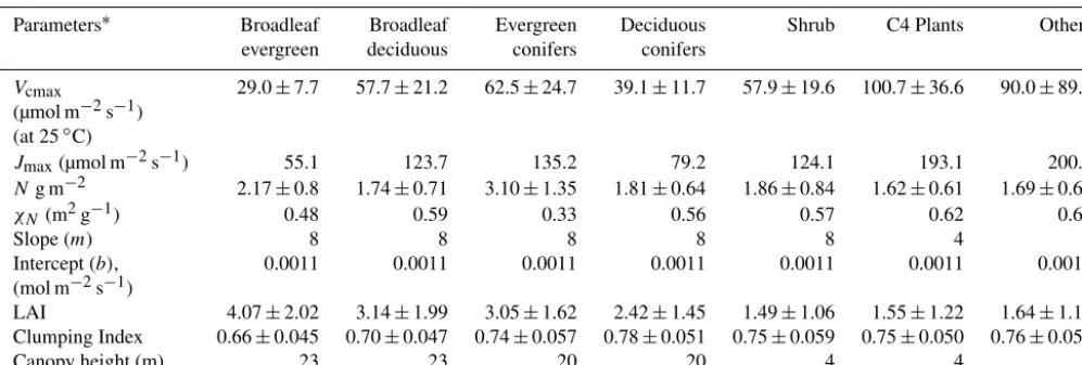
Table 1.Biophysical parameters are assigned by plant functional types in BEPS. References for the chosen values of these parameters are found in Chen et al. (2012).

Parameters∗ Broadleaf Broadleaf Evergreen Deciduous Shrub C4 Plants Others evergreen deciduous conifers conifers

Vcmax

(µmol m−2s−1) (at 25◦C)

29.0±7.7 57.7±21.2 62.5±24.7 39.1±11.7 57.9±19.6 100.7±36.6 90.0±89.5

Jmax(µmol m−2s−1) 55.1 123.7 135.2 79.2 124.1 193.1 200.0

Ng m−2 2.17±0.8 1.74±0.71 3.10±1.35 1.81±0.64 1.86±0.84 1.62±0.61 1.69±0.69

χN(m2g−1) 0.48 0.59 0.33 0.56 0.57 0.62 0.60

Slope (m) 8 8 8 8 8 4 8

Intercept (b), (mol m−2s−1)

0.0011 0.0011 0.0011 0.0011 0.0011 0.0011 0.0011

LAI 4.07±2.02 3.14±1.99 3.05±1.62 2.42±1.45 1.49±1.06 1.55±1.22 1.64±1.15 Clumping Index 0.66±0.045 0.70±0.047 0.74±0.057 0.78±0.051 0.75±0.059 0.75±0.050 0.76±0.059

Canopy height (m) 23 23 20 20 4 4 4

∗_V

cmaxis the leaf maximum carboxylation rate at 25◦C,Jmaxis the maximum electron transport rate,Nis the leaf nitrogen content,χNis the slope ofVcmaxvariation withN, andmandbare the slope and intercept in the Ball–Berry equation. The peak growing season LAI and clumping index are given as the mean and standard deviation for each plant functional type.

is the respiration rate occurring during the day not related to photorespiration;0is the CO2compensation point in the

absence ofRd; andJ is the rate of photosynthetic electron

transport. These parameters are the same as those used in computing the CO2flux.

Our methods of computing stomatal and mesophyll con-ductances differ from previous studies (Suits et al., 2005; Scholze et al., 2008; Rayner et al., 2008) in the following ways: (1) these conductances are calculated separately for sunlit and shaded leaves because BEPS is a two-leaf model, in which the total GPP of a canopy is taken as the sum of sun-lit and shaded leaf GPP, and (2) the mesophyll conductance mechanistically depends on a set of parameters rather than being treated as a constant or to be proportional to the stom-atal conductance. Since it has been demonstrated that sunlit and shaded leaf separation is essential for accurate modelling of canopy-level photosynthesis (Chen et al., 1999; Sprintsin et al., 2011), it is expected that this separation is also es-sential for 13CO2flux estimation. We found that the use of

Harley’s method for computing the mesophyll conductance makes the calculated 13C photosynthetic fractionation sta-ble for its global application, while the simpler method of treating the mesophyll conductance in proportion with the stomatal conductance often incurs abnormally large or small values of13C photosynthetic fractionation.

The photosynthetic13CO2 flux is in disequilibrium with

the respiratory 13CO2 flux because of the change in

at-mospheric13CO2concentration since the preindustrial time

(Ciais et al., 1995b; Fung et al., 1997). The heterotrophic res-piratory flux from the decomposition of organic matter of different ages carries the memory of the past atmospheric

13_CO

2 concentration, while the photosynthetic 13CO2 flux

is affected by the current atmospheric13CO2concentration.

Table 2.Global average ages of soil carbon pools computed by BEPS with consideration of the influences of temperature and soil moisture on the decomposition rates of these pools.

Soil carbon Name Global average age

pooli τi(year)

1 Surface structural leaf litter

5.0

2 Surface metabolic leaf litter

2.3

3 Soil structural litter 4.4 4 Soil metabolic litter 2.3

5 Woody litter 34.9

6 Surface microbe 11.1

7 Soil microbe 28.5

8 Slow carbon 35.5

9 Passive carbon 667.9

The isotopic composition of each of the nine soil carbon pools (δ13Csoil,i)is estimated with following formula: δ13Csoil,i=δ13Ca(2003−τi)−εlph, (16)

whereδ13Cais the isotopic composition of carbon in

atmo-spheric CO2in the past as determined by the ice-core record

(Francey et al., 1999),εlphis the annual mean of

photosyn-thetic discrimination in 2003 andτi is the age of carbon pool i (Table 2) (Ju and Chen, 2005). In the calculation of the mean age of a carbon pool, we have considered the ages of various carbon pools at the time of entering the pool (Potter et al., 1993) so that the mean age is considerably larger than the turnover time determined by the decomposition rate (Fung et al., 1997). The meanδ13Csoil is taken as the flux-weighted

for the globe are shown in Fig. 5. The 13C composition of the biosphere δlb in Eq. (8) is taken as the mean δ13Csoil,

while the biospheric13C compositionδ_lbe in equilibrium with the current atmosphere is taken asδa−εlph.

The accuracy of the BEPS model in simulating atmo-spheric 13CO2 concentration was previously tested (Chen

et al., 2006; Chen and Chen, 2007) against measure-ments over a boreal forest at Fraserdale, Ontario, Canada (49◦52029.900N, 81◦34012.300W). Flask measurements of δ13Ca were made 40 times in both daytime and nighttime

on a tower at a height of 20 m during a 3-day campaign on 21–23 July 1999. BEPS simulated these measurements with RMSE=0.34 ‰ andr2=0.76.

2.3 Transport modelling

A transport-only version of the atmospheric chemistry and transport model TM5 (Krol et al., 2003, 2005) is used for CO2 and13CO2transport modelling to produce a fully

lin-ear operator on these fluxes. The spatial resolution of TM5 is 6◦×4◦for the globe and 3◦×2◦for North America, and the atmosphere is divided vertically into 25 layers with 5 lay-ers in the planetary boundary layer. Tracer transport (advec-tion, vertical diffusion, cloud convection) in TM5 is driven by offline meteorological fields taken from the European Cen-tre for Medium Range Weather Forecast (ECMWF) model. All physical parameterizations in TM5 are kept the same as the ECMWF formulation to achieve compatibility between them. The four background fluxes from terrestrial ecosys-tems, oceans, fossil-fuel burning and biomass burning are individually inputted to TM5 to calculate the contributions of these fluxes to the atmospheric CO2 and13CO2

concen-trations. Since the main purpose of this study is to develop a joint inversion system, only one transport model is used, the transport matrixMis assumed to be free of errors.

2.4 CO2and13CO2data sets

Monthly CO2 and 13CO2 concentration data from 2000 to

2004 are compiled from the GLOBALVIEW CO2and13CO2

database. Though the GLOBALVIEW database consists of both extrapolated and interpolated data that were created based on the technique devised by Masarie and Tans (1995), we selected the synchronized and smoothed values of actual observations to compile our concentrations data sets. Only direct measurements of CO2from the GLOBALVIEW data

set are used in our inversion after using a time-frequency weighting scheme (Deng and Chen, 2011). There are 5431 monthly data from 209 sites for 42 months used for CO2

(5431 out of 8778, i.e. 209×42), and 3066 monthly data from 73 sites for 13CO2(i.e. 73×42 monthly data). Since

the number of13CO2observation sites is much smaller than

that of CO2 sites, all monthly data at 73 sites are used for

13_CO

2, and the missing13CO2data are filled with the

refer-ence data provided in the same GLOBALVIEW data set. The

filled data may have introduced an additional error to the data set as shown in Fig. 15b.

To minimize the non-linear aggregation effects of the large regions (Pickett-Heaps, 2007), the contributions of the four background fluxes are subtracted from the above monthly concentrations. So the matrix c in Eqs. (3) and (4) is ex-pressed as

c=cobs−cff−cbio−cocn−cfire, (17)

wherecobsis the monthly CO2and13CO2concentrations

ob-tained from GLOBALVIEW, andcff,cbio,cocn andcfireare

simulated contributions of CO2 and13CO2 concentrations

from the terrestrial biosphere, ocean, fossil-fuel and fire fluxes, respectively.

3 Results

3.1 Prior CO2and13CO2fluxes

Terrestrial ecosystem models integrate many sources of in-formation, including vegetation structure, soil and meteorol-ogy, to estimate carbon exchange of the land surface with the atmosphere. Prior CO2 and13CO2 fluxes produced by

a model can therefore provide indispensable constraints to the otherwise ill-posed inversion based on CO2and13CO2

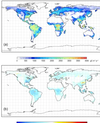
concentration observations alone. Depending on the assigned relative magnitudes of the error matrixes of these observa-tions and these prior fluxes (i.e. RandQ in Eq. 3), these prior fluxes can have equal or even dominant importance to these observations in the inversion results. We have there-fore paid a great attention in modelling these prior fluxes, in order to minimize the total inversion errors. Figure 2a shows an example of the global terrestrial GPP distribution in 2003 modelled by BEPS. The total GPP in this year is 132±22 Pg C year−1(Chen et al., 2012). This value is larger than some of the recent estimates, such as 123 Pg C year−1 by Beer et al. (2010), mostly because the LAI values used as input to BEPS are generally larger than those of the MODIS product (Garrigues et al., 2008). Our LAI values are larger because we used a global clumping index map derived from a multi-angle satellite sensor POLDER (Chen et al., 2005). Clumping increases shaded leaves, which contributed about 35 % to the total GPP globally. Without considering this clumping effect, the shaded leaf area is underestimated re-sulting in an underestimation of the global GPP by 9 % (Chen et al., 2012). As the spatial distribution of clumping is not uniform (boreal and tropical forests are most clumped and crops and grasses are least clumped), this refinement in the GPP spatial distribution would have some effects on the in-version results between regions.

Figure 2. (a)Gross primary productivity (GPP) distribution in 2003 computed using remote sensing LAI and land cover maps and climate and soil data, and(b)net ecosystem productivity (NEP) distribution in 2003. Both are calculated using the BEPS model. Annual NEP maps from 2000 to 2004 are used to as the prior flux in the inversions. This GPP map is used to distribute the flux uncertainty among the 39 land regions.

smaller (globally 2 Pg C year−1by BEPS) because a model spin-up approach is used to estimate the soil carbon pool sizes based on a dynamic equilibrium assumption. Under this assumption, the annual heterotrophic respiration (Flb)equals

annual NPP during the preindustrial period, and the soil car-bon pool sizes are derived fromFlbby solving a set of

dif-ferential equations describing the decomposition and inter-actions among the pools (Govind et al., 2011). In this way, Flbis forced to depend on NPP and the systematic biases in

GPP are not carried into NEP estimation. NEP is non-zero af-ter the preindustrial period because of the changes in climate and atmospheric composition (CO2and nitrogen) as well as

disturbance. In our regional modelling, both disturbance and

non-disturbance effects are considered for Canada (Chen et al., 2003) and USA (Zhang et al., 2012) forests. However, in our global model spin-up from 1901 (taken as the end of preindustrial period) to 2000, only the non-disturbance ef-fects are considered because of lack of spatially explicit dis-turbance data outside of North America, while carbon emis-sion due to fire disturbance in the study period from 2000 to 2004 is considered separately using the GFED data set (Ran-derson et al., 2007; van der Werf et al., 2006). The prior net CO2fluxes for the globe for the years 2002–2004 are given

Table 3.Inverted fluxes (Pg C year−1), averaged for 2002–2004, for land and ocean regions with (CO2+13CO2)and without (CO2-only)13C

constraint. The negative sign denotes the flux from the atmosphere to the surface (sink). Various treatments are made to13C discrimination and disequilibrium fluxes represented by the following cases. Case I: full consideration of the regional differences in discrimination and disequilibrium; case II: same as case I, but the annual photosynthetic discrimination ratio is set at a constant of−14.1 ‰, although it is monthly variation pattern as modelled by BEPS is retained; case III: same as case I, but the disequilibrium flux over land is ignored; case IV: same as case I, but the disequilibrium flux over ocean is ignored; case V: same as case I, but the disequilibrium flux over both land and ocean is ignored.

Inverted CO2flux

Double CO2data CO2+13CO2data

decon-Region Prior flux volution Case I Case II Case III Case IV Case V

Land −2.61±2.07 −2.90 −3.40±0.84 −2.53±0.93 −2.49±0.95 −3.58±0.93 −2.66±0.93 −3.71±0.93 Ocean −2.13±0.67 −2.36 −1.48±0.40 −2.36±0.49 −2.35±0.48 −2.24±0.49 −4.44±0.49 −4.32±0.49

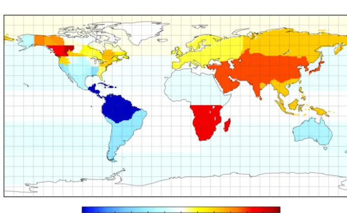
Figure 3.The annual mean of the total photosynthetic13C discrimination (1in Eq. 7) in 2003.

The global distribution of the total photosynthetic discrim-ination (δ13Cpt=δ13Ca−1) modelled by BEPS is shown

in Fig. 3. Forests, such as those in North America, Russia, Europe, Amazon, central Africa, central China and southeast Asia, generally have high photosynthetic discrimination rates (>16 ‰), whereas grassland and cropland (in particular C4 grasses and crops) have low discrimination rates. Also shown in Fig. 3 is the ocean diffusive discrimination against13CO2.

The discrimination over ocean is much smaller than that over land. This difference between land and ocean discrimination may be considered as the largest signal of 13CO2

observa-tions on the global carbon cycle (Tans et al., 1990; Rayner et al., 2008) and is considered in our inversion using different

13_CO

2 discrimination rates for ocean and land regions (see

Eq. 6).

To estimate the disequilibrium between photosynthetic and respiratory discrimination against13CO2, the global

dis-tribution of the mean soil carbon age is computed after weighting the ages of the nine soil carbon pools against their fluxes due to decomposition (Fig. 4). Forests at high lati-tudes have the soil carbon age of about 40–60 years, while the tropical forests have much lower values in the range from 10 to 30 years. This latitudinal distribution pattern is mostly determined by soil temperature. In low latitudes, high tem-perature induces fast turnovers of detritus and fast soil car-bon pools, whereas at high latitudes, low temperature main-tains relatively large fractions of slow and passive soil car-bon pools. Cropland and grassland also have larger fractions of fast and detritus carbon pools than forest cover types and therefore have younger soil carbon on average. This spatial distribution of soil carbon age has a strong influence on the total respiratory discrimination against 13C (δ13Cr)

Figure 4.Global distribution of the flux-weighted mean age of soil carbon pools (Eq. 8).

Figure 5.Globalδ13C distribution over land (annual flux-weighted average in 2003).

less13CO2concentration and hence has lower discrimination

rates (largerδ13Cror smaller absolute value). However,

res-piration would mostly depend on the photosynthetic discrim-ination rates as soil organic matter originates from photosyn-thetic production. As a result, forested areas have higher res-piratory discrimination rates (lowerδ13Cror larger absolute

value). Most of the high values ofδ13Crin Fig. 5 are

associ-ated with large fractions of C4 plants in the grid, such as the corn belt in the USA, cropland in northeastern China, south-ern border of Sahara desert and southeastsouth-ern South America. The global distribution of the disequilibrium between photo-synthetic and respiratory discrimination, taken as the differ-ence between Fig. 3 and 5, is shown in Fig. 6. The disequi-librium is the largest at high-latitude boreal forests in North

America and Eurasia because their soil carbon is the oldest, as shown in Fig. 4. The spatial distribution pattern of the dise-quilibrium is similar to those of Ciais et al. (1995b) and Fung et al. (1997) but the magnitude is larger because the date of our result in 2000 are more recent than these two previous studies. As the time lapses, the atmosphere is getting lighter in terms of the isotopic composition of CO2resulting from

the increased air-borne CO2 from fossil-fuel consumption.

Also shown in Fig. 6 is the disequilibrium over the ocean es-timated using the method of Ciais et al. (1995b). This ocean disequilibrium has a large latitudinal gradient because of the gradients in sea surface temperature gradient and the fluxes of CO2 and13CO2. The spatial distribution in the

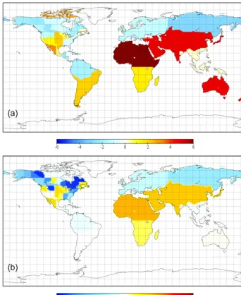
Figure 6.Disequilibria between13C fluxes to and from the land or ocean surface in 2000. At the land surface, the disequilibrium is the differ-ence between photosynthetic and respiratory discriminations against13C, and at the ocean surface it is the difference in13C discrimination between the one-way diffusive downward and upward fluxes.

and land may be considered to be the secondary signal of

13_CO

2 observations on the global carbon cycle. The effects

of these disequilibria on the carbon flux are considered in our inversion through pre-subtracting their contributions to the measured13CO2composition in Eq. (10).

3.2 Inverse modelling results

Although the inversions were made for the 2000–2004 pe-riod, the results of the first 2 years are not included in the analysis because they are affected by the assumption of uni-form global distributions of CO2and13CO2concentrations

at the start of our transport modelling using TM5. An 18–24-month period is usually considered to be necessary for the simulated distributions to reach realistic states with reason-ably accurate prior surface fluxes from ocean and land and atmospheric transport simulations (Rödenbeck et al., 2003; Deng and Chen, 2011). The following results are therefore summarized as the average for the 2002–2004 period.

3.2.1 Partition between ocean and land sinks with and without13CO2constraint

To investigate the usefulness of13CO2 observations in

par-titioning between ocean and land sinks, we conducted in-versions with and without13CO2constraint as expressed in

Eq. (6), i.e. with and without the13C-related expansions of the matrixes. The CO2-only inversion increases the land sink

from the prior of 2.61–3.40 Pg C year−1while decreasing the ocean sink from the prior of 2.13–1.48 Pg C year−1(Table 3). These results are similar to those of Deng and Chen (2011). The results from the joint inversion are considerably

differ-ent; the posterior sinks for land and ocean become 2.53 and 2.36 Pg C year−1(Table 3), respectively, suggesting that the use of13CO2observations in the inversion considerably

in-fluenced the partition between land and ocean fluxes. The ra-tio between land and ocean sinks is 1.07. The joint inversion system developed in this study may be regarded as a differ-ent form of double deconvolution. Using the double decon-volution method with the global average disequilibrium co-efficients of 0.49 and 0.78 ‰ and the disequilibrium fluxes of 26.8 and 66 Pg C year−1‰ for land and ocean derived in this study (Table 4), respectively, we also calculated the land and ocean sinks to be 2.90 and 2.36 Pg C year−1, respec-tively. The ratio between land and ocean sinks is 1.23, which is close to the value of 1.07 derived from the joint inversion system, indicating that the joint inversion can effectively per-form double deconvolution. Our joint inversion system dif-fers from previous double deconvolution systems (Siegen-thaler and Oeschger, 1987; Keeling et al., 1989a; Francey et al., 1995; Randerson et al., 2002) in the following ways: (1) the estimation of CO2 fluxes for the land and ocean is

additionally constrained by the prior fluxes for the land and ocean rather than being entirely dependent on measured CO2

concentration and 13CO2 composition, and (2) the

spatio-temporal variations in all parameters associated with isotopic discrimination and disequilibrium are considered in the esti-mation of the CO2flux using a mechanistic biospheric model

Table 4.Comparison of land and ocean disequilibrium coefficients and disequilibrium fluxes calculated in this study with those in previous studies.

Land Land dis- Ocean Ocean dis-disequilibrium equilibrium flux disequilibrium equilibrium flux Studies Year coefficient (‰ ) (Pg C year−1‰) coefficient (‰) (Pg C year−1‰ )

This study 2002–2004 0.49 26.8 0.78 66

Fung et al. (1997) 1988 0.33 N/A N/A N/A

Randerson et al. (2002) 1981–1994 0.33 20 0.6 55 Alden et al. (2010) 1991–2007 0.45–0.61 22.7–30.6 N/A 92.3–100.2 (globe total) Van der Velde et al. (2013) 1991–2007 0.486 25.4 N/A 48.7 Francey et al. (1995) 1987 0.43 25.8 0.48 43.8

Table 5.Global isotopic mass budgets averaged for the 2002–2004 period for the prior, double deconvolution, CO2-only inversion, and joint

inversion (unit: Pg C year−1‰). Also shown are ocean and land net fluxes (unit: Pg C year−1)for these cases for comparison purposes. For the prior fluxes, the component of each flux are indicated in the parentheses. The isotopic coefficients are same among the cases.

Double CO2- Joint

Isotopic terms Prior deconvolution only inversion inversion

−Cad(δa)/dt 15.0 [750 Pg C×(−0.02 ‰ year−1)] 15.0 15.0 15.0 Ff(δf−δa)∗ −153.7 [8.9 Pg C year−1×(−17.27 ‰)] −153.7 −153.7 −153.7

−(Flph−Flb)εlh 36.7 [2.6 Pg C year−1×(−14.10 ‰ )] 40.9 47.9 39.5

Flb(δlb−δlbe) 26.8 [54.7 Pg C year−1×(−0.49 ‰ )] 26.8 26.8 26.8

−(Fao−Foa)εao 4.2 [2.1 Pg C year−1×(−2.00 ‰ )] 4.8 3.0 4.6

Foa(δeoa−δoa) 66.0 [84.6 Pg C year−1×(−0.78 ‰ )] 66.0 66.0 66.0

Global Budget −5.0 0.8 −5.0 1.8

(Flph−Flb), (Pg C year−1) −2.6 −2.9 −3.4 −2.8 (Fao−Foa)(Pg C year−1) −2.1 −2.4 −1.5 −2.3

∗_F

fis the carbon emission from fossil fuel and biomass burning, 6.9 and 2.1 Pg C year−1, respectively, andδfis weighted average13C composition for fossil fuel and biomass burning, being 25.27 ‰, andδa= −8.0‰.

The impacts of13CO2data on the joint inversion can also

be evaluated from the view point of global13CO2mass

bud-get. Table 5 shows the budgets and its components for the prior, double deconvolution, CO2-only inversion and joint

in-version cases. In these cases, the isofluxes due to fossil-fuel emission, land and ocean disequilibrium and atmospheric storage change are the same, and only those due to discrimi-nation over land and ocean are adjusted. The prior case shows a global imbalance of −5.0 Pg C year−1‰, indicating that either the prior land or ocean fluxes or both are inconsis-tent with13CO2measurements. Through double

deconvolu-tion, this imbalance is greatly reduced to 0.8 Pg C year−1‰, mostly by an increase in the discrimination flux over land because of its large discrimination rate. The CO2-only

inver-sion increases the land discrimination flux while decreasing the ocean discrimination flux, resulting in no improvement in the global isotopic balance. The joint inversion optimized both ocean and land fluxes in the direction consistent with

13_CO

2 measurements, reducing the imbalance considerably

to 1.8 Pg C year−1‰. These cases illustrate clearly that the global isotopic mass balance is very sensitive to the partition between ocean and land fluxes because of the large

differ-Figure 7.Comparison of land and ocean carbon sinks derived from inversions with and without the13CO2constraint against the Global

Carbon Project results (Le Quéré et al., 2013).

ence in the discrimination rate between land and ocean. In this analysis, the disequilibrium fluxes are not adjusted,

Existing estimates for the ocean sink for anthropogenic CO2in the 2000s varies from 1.94 to 2.6 Pg C year−1

(Wan-ninkhof et al., 2013; Landschützer et al., 2014; Majkut et al., 2014; DeVries, 2014). The average ocean sink for the 2002–2004 period summarized by the Global Carbon Project (GCP) (Le Quéré et al., 2013) is 2.4 Pg C year−1, while the land sink in the same period is 2.7 Pg C year−1as the resid-ual of the global carbon budget after including the emission due to land use change as a source of carbon. Although the prior estimates of these sinks in our inversions are similar to these values, our CO2-only inversion considerably increases

the land sink and decreases the ocean sink. The addition of

13_CO

2measurements to the inversion significantly decreases

the land sink and increases the ocean sink, pulling the in-version results in the direction to agree with these existing estimates (Fig. 7). This may indicate that the use of 13CO2

measurements in the joint inversion has improved the CO2

estimation. In this comparison, we have not considered the unknown small amount (0.1–0.3 Pg C year−1)of lateral car-bon transport in rivers from land to ocean. This amount is included in some of the estimates of the ocean sink used by GCP, and therefore should be subtracted from the ocean sink and added to the land sink by GCP in order to compare with our atmospheric inversion results.

3.2.2 Influence of13CO2constraint on the spatial distribution of the inverted carbon flux

The 13CO2 constraint modified not only the partition

be-tween ocean and land fluxes but also their spatial distribution patterns. Figure 8 shows the result of the CO2-only

inver-sion (i.e. without the13CO2constraint), as the net carbon flux

over land and ocean averaged for the period of 2002–2004. Figure 9 shows the difference between inversions with and without the13CO2constraint, i.e. the result of CO2+13CO2

inversion minus that of CO2-only inversion. The general

pat-terns of the inverted carbon flux are similar between these two inversions because these inversions depend primarily on the CO2concentration, the prior flux, the error matrixes

of the prior flux, and concentration observations. However, there are several large or notable differences: (1) the Amazon region (region 31) is changed from a carbon source to a sink (Fig. 10; note: a reduction in sources is shown as a negative value); (2) the carbon sink in the tropical Asia (region 37) is noticeably reduced (by about 10–20 g C m−2year−1from a sink magnitude of about 80–100 g C m−2_year−1_{); (3) the}

sink in Asia (region 36) decreases pronouncedly by about 10–20 g C m−2year−1, while the sinks in Russia (region 35) and Europe (region 39) are also reduced by some extents (about 5–20 g C m−2year−1); (4) most small regions in the southern part of North America show increases in sinks, but those in the northern part (Canada and Alaska) show in-creases in sources (see also Fig. 11); the overall sink in North America decreases from 0.67 to 0.54 Pg C year−1(Fig. 10);

and (5) most ocean regions at mid-latitudes have small gains in sink.

It is of particular importance to note that the 13CO2

constraint changed the Amazon region from a carbon source of 0.43±0.46 Pg C year−1 to a carbon sink of 0.08±0.38 Pg C year−1with a notable reduction in the pos-terior uncertainty, which is higher than uncertainty reduc-tions in most other regions (Fig. 10). This change is likely caused by the relatively large addition of information from

13_CO

2 in this tropical region where CO2 observations are

sparse, causing large uncertainties in the inverted flux in this region in the CO2-only inversion. Potter et al. (2009)

sim-ulated the NEP of the Amazon region using the Carnegie– Ames–Stanford Approach driven by remote sensing inputs and found that the NEP for the region was slightly negative (−0.07 Pg C year−1)over the 2000–2004 period. Davidson et al. (2012) summarized from various inventory-based stud-ies that mature forests in the region were accumulating car-bon at a rate of 0.29–0.57 Pg C year−1over the decade before 2005, meaning that NEP is positive. Since the fire emission is estimated to be 0.50 Pg C year−1(Richey et al., 2002), the Amazon region would be either a net source of carbon or about carbon neutral. Since spatially explicit fire emission is considered together with fossil-fuel emission as a source in our study, the inverted carbon flux corresponds to−NEP, and therefore the result from our joint inversion is in broad agree-ment with the results of Potter et al. (2009) and Davidson et al. (2012). Without the13CO2constraint, our inversion result

shows an unreasonably large source of carbon in the Amazon region.

3.2.3 Influence of the spatial distribution of photosynthetic discrimination on the inverted carbon flux

The joint inversion results shown in Figs. 9–11 are from case I with the best estimates of the13C discrimination and dis-equilibrium fluxes and therefore represent a baseline study to which other cases are compared for the purpose of in-vestigating the importance of accurate consideration of the spatial distributions of isotopic discrimination and disequi-librium over land and ocean. Case II is designed to investi-gate the importance of considering the spatial distribution of the photosynthetic isotopic discrimination over land for in-verting the CO2flux by fixing the discrimination at a constant

over land. Figure 12a shows the spatial distribution of the dif-ference in the total isotopic discrimination, i.e.Dj=εlph,j, among 39 land regions between case I and case II, calcu-lated as case I minus case II. Regions with positive differ-ences in Dj are shown with positive differences in the in-verted CO2 flux (Fig. 12b), meaning larger sinks (negative

values) in case II, and vice versa. This is because a smaller discrimination rate (smaller than−14.1 ‰) means a larger CO2flux from the atmosphere to the surface (more negative

Figure 8.Global distribution of inverted CO2flux using CO2data only (2002–2004 average).

Figure 9.Difference of the inverted CO2flux between using CO2+13CO2data and using CO2data only (2002–2004 average).

atmosphere. Under the same condition, a larger discrimina-tion induces a smaller sink (less negative). The absolute re-gional differences between case I and case II are considerable (Fig. 12b), e.g. up to 18 g C m−2year−1, showing increases in sinks in Africa, Asia and Australia and decreases in sinks in Amazon, Europe, Russia and most of the small regions in North America. However, the total global sink values of case II after ignoring the spatial distribution of the disequilibrium rate over land change very little from those of case I (Ta-ble 3): from 2.53±0.93 to 2.49±0.95 Pg C year−1for land and from 2.36±0.49 to 2.35±0.48 Pg C year−1for ocean. This is because the global mean discrimination rates are the same between these two cases.

3.2.4 Influence of the uncertainties in disequilibrium fluxes on the inverted carbon flux

The average disequilibrium coefficients and fluxes for land and ocean derived in this study are comparable to pub-lished results (Table 4), although the estimates of the dis-equilibrium flux over ocean in previous studies vary in a large range. The uncertainty in the estimated land and ocean disequilibrium fluxes mainly arises from two sources: the estimated disequilibrium coefficient and one-way CO2

flux from the surface. Mathematically, the total uncertainty in the disequilibrium flux, denoted as 1(δ·F ), equals

p

Figure 10.Comparison between inversion results with and without13CO2constraint for 21 regions of the globe for the periods of 2002–2004.

Figure 11.Comparison between inversion results with and without13CO2constraint for 30 regions in North America.

on the modelled mean soil carbon age by BEPS, which is estimated to be ±5 years, causing an error in the disequi-librium coefficient to be±0.11 ‰ based on the slope ofδa

against time at about 1979 (the flux-weighted global mean soil carbon age is 24 years). The second source is estimated to be 9.5 Pg C year−1in NPP, which is taken as 45 % of the error in GPP, i.e. 21 Pg C year−1(Chen et al., 2012). With NPP=59.4 Pg C year−1 and the mean disequilibrium effi-cient of 0.49 ‰, the uncertainty in the estimated land disequi-librium flux is therefore p(0.11×59.4)2_+(0.49×9.5)2₌

8.0 Pg C year−1_{‰. For ocean, the error in the modelled}

dis-equilibrium coefficient is mostly caused by sea surface tem-perature (SST), if the coefficients in the equation developed by Ciais et al. (1995b) are assumed to be accurate. With an error of 1.0 K in SST, the error in the calculated global average disequilibrium coefficient is±0.12 ‰. The error in the one-way ocean flux is difficult to estimate, but we use the value of 10 Pg C year−1 inferred from the global iso-topic budget uncertainty by Alden et al. (2010). Their in-ferred range of the ocean disequilibrium flux is from 92.3 to 100.2 Pg C year−1‰, and we use our disequilibrium coef-ficient of 0.78 ‰ to calculate this one-way flux uncertainty. Based on the OPA–PISCES-T model, the one-way flux from

ocean to atmosphere is 84.6 Pg C year−1, and the uncer-tainty in the estimated ocean disequilibrium flux is therefore

p

(0.12×84.6)2_+(0.78×10)2_{=12.7 Pg C year}−1_‰.

Case III, case IV and case V are conducted to investigate the relative importance of the disequilibrium fluxes over land and ocean (Table 3) in the CO2 flux inversion. In case III,

where the disequilibrium over land is ignored while other settings remain the same as case I, the land sink increases by 1.05 Pg C year−1, whereas the ocean sink decreases by 0.08 Pg C year−1_{in comparison with case I. When the}

dise-quilibrium over ocean is ignored instead (case IV), the land sink increases by 0.13 Pg C year−1, while the ocean sink increases by 2.08 Pg C year−1, in comparison with case I. When the disequilibria over both land and ocean are ignored, the land sink increases by 1.18 Pg C year−1, while the ocean sink increases by 1.96 Pg C year−1, in comparison with case I. Results from these case studies suggest that in the joint inversion using both CO2and13CO2measurements, the

in-verted CO2flux can be significantly influenced by the

dise-quilibrium fluxes of land and ocean. The carbon sinks over land and ocean increase when these disequilibrium fluxes are ignored because the photosynthetic and diffusive sources of

13_CO

ig-Figure 12. (a)Difference inεlph(‰) and(b)the inverted CO2flux (g C m−2year−1)between case I and case II, i.e. Case I minus case II.

See Sect. 2.1.3 for the description of these cases.

noring the disequilibrium sources. These pronounced influ-ences of the disequilibrium fluxes on the CO2sink inversion

suggest that13CO2data contain strong signals for the global

carbon cycle. In the joint inversion, these data can have the power to distort the global CO2 mass balance if the13CO2

mass budget (Eq. 8) is not properly simulated. The influence of13CO2on the joint inversion depends only weakly on the

estimated uncertainty in the13CO2data. We found that if the

uncertainty is reduced by half, the sum of the land and ocean sink deviates from the CO2-only case by 2–6 % for all

sce-narios, suggesting that the mean disequilibrium fluxes play the dominant roles in the joint inversion.

The impacts of these disequilibrium fluxes on the inverted CO2flux determined in case III, case IV and case V are

sim-ilar to previous results using the double deconvolution

tech-nique (Tans et al., 1993; Ciais et al., 1995b; Randerson et al., 2002). However, the influences of these disequilibrium fluxes on the joint inversion could possibly be compromised due to the small number of13C observation sites relative to the num-ber of CO2observation sites used in the joint inversion. The

number of linear equations for CO2concentration in our joint