www.geosci-model-dev.net/9/3111/2016/ doi:10.5194/gmd-9-3111-2016
© Author(s) 2016. CC Attribution 3.0 License.
Improved representations of coupled soil–canopy processes in the
CABLE land surface model (Subversion revision 3432)
Vanessa Haverd1, Matthias Cuntz2, Lars P. Nieradzik1, and Ian N. Harman1
1CSIRO Oceans and Atmosphere, P.O. Box 3023, Canberra ACT 2601, Australia
2Department Computational Hydrosystems, UFZ – Helmholtz Centre for Environmental Research, Permoserstr. 15,
04318 Leipzig, Germany
Correspondence to:Vanessa Haverd ([email protected])
Received: 14 February 2016 – Published in Geosci. Model Dev. Discuss.: 26 February 2016 Revised: 21 July 2016 – Accepted: 22 July 2016 – Published: 7 September 2016
Abstract. CABLE is a global land surface model, which has been used extensively in offline and coupled simulations. While CABLE performs well in comparison with other land surface models, results are impacted by decoupling of tran-spiration and photosynthesis fluxes under drying soil con-ditions, often leading to implausibly high water use effi-ciencies. Here, we present a solution to this problem, en-suring that modelled transpiration is always consistent with modelled photosynthesis, while introducing a parsimonious single-parameter drought response function which is coupled to root water uptake. We further improve CABLE’s simula-tion of coupled soil–canopy processes by introducing an al-ternative hydrology model with a physically accurate repre-sentation of coupled energy and water fluxes at the soil–air interface, including a more realistic formulation of transfer under atmospherically stable conditions within the canopy and in the presence of leaf litter. The effects of these model developments are assessed using data from 18 stations from the global eddy covariance FLUXNET database, selected to span a large climatic range. Marked improvements are demonstrated, with root mean squared errors for monthly la-tent heat fluxes and water use efficiencies being reduced by 40 %. Results highlight the important roles of deep soil mois-ture in mediating drought response and litter in dampening soil evaporation.
1 Introduction
In many global terrestrial carbon-cycle models, global gross primary production (GPP) and net biome production (NBP) are over-sensitive to precipitation anomalies. This was re-ported by Piao et al. (2013) and highlighted in the IPCC 5th Assessment Report (Ciais et al., 2013): “Terrestrial car-bon cycle models used in AR5 generally underestimate GPP in the water limited regions, implying that these models do not correctly simulate soil moisture conditions, or that they are too sensitive to changes in soil moisture (Jung et al., 2007). Most models [. . . ] estimated that the interan-nual precipitation sensitivity of the global land CO2 sink
to be higher than that of the observed residual land sink (−0.01 PgC yr−1mm−1; [. . . ]).”
CABLE (Subversion revision 3432) is the land surface scheme in the ACCESS earth system model (Kowalczyk et al., 2013; Law et al., 2015), as used in the IPCC 5th As-sessment report (Ciais et al., 2013), and is one of an ensem-ble of ecosystem and land-surface models contributing to the Global Carbon Project’s TRENDY initiative (Ahlström et al., 2015; Sitch et al., 2015). While CABLE2.0 performs well in comparison with other land surface models (e.g. Best et al., 2015), results suggest an over-sensitivity of evapotranspira-tion to drought (Best et al., 2015), and may be impacted by decoupling of transpiration and photosynthesis fluxes under drying soil conditions (Wang et al., 2011), potentially leading to implausibly high water use efficiencies.
respec-tively). Both studies noted an over-sensitivity of ET to water availability in CABLE with the standard drought response setting. Li et al. (2012) implemented an alternate stomatal drought response function based on the parameterization of Lai and Katul (2000), along with a parameterization for hy-draulic redistribution (Ryel et al., 2002) and demonstrated marked improvements at three FLUXNET sites, largely at-tributable to the introduction of hydraulic redistribution.
De Kauwe et al. (2015a) applied alternative soil moisture deficit responses to stomatal conductance and photosynthetic capacity, based on the formulations of Zhou et al. (2013). Im-provements were demonstrated at five European FLUXNET sites, with model performance dependent on a site-specific drought tolerance parameter. Modification to the vapour-pressure deficit response of stomatal conductance in CABLE (De Kauwe et al., 2015b; Kala et al., 2015, 2016) has also been featured in recent studies, but it is evident that deficien-cies in the predictions of seasonal cycles of evaporation are not resolved by this modification (De Kauwe et al., 2015b; Fig. 3). Recently Decker (2015) introduced to CABLE new conceptual parameterizations of subgrid-scale soil moisture, runoff generation, and groundwater, and showed improved performance against observation-based estimates of global ET, without modifying CABLE’s vegetation response to soil moisture.
Haverd et al. (2013) proposed an alternative formula-tion for coupled drought response and root water extrac-tion in CABLE, operating in tandem with an alternative soil hydrology scheme called SLI (Haverd and Cuntz, 2010). In that work, CABLE, constrained by multiple observation types, was applied to a high-resolution (0.05◦×0.05◦) as-sessment of the Australian terrestrial carbon and water cy-cles. Here, the constrained model, including an alternative drought response, performed well against eddy-covariance-based flux estimates, and in particular replicated the observed sustained evapotranspiration through seasonal drought peri-ods in drought-adapted savanna ecosystems.
In this work, we take lessons learnt from the Australian re-gional application (Haverd et al., 2013) and apply them to the global context. In particular, we seek to resolve in CABLE2.0 the problems of over-sensitivity of ET to drought and decou-pling of transpiration and photosynthesis fluxes under drying soil conditions. Firstly, we introduce the alternative drought-response of Haverd et al. (2013) as an option in CABLE2.0, making use of global data on maximum vegetation rooting depth (Canadell et al., 1996), and ensuring that photosynthe-sis is limited by extractable soil moisture. Since a significant component of ET can be soil evaporation, we secondly im-prove the physical accuracy of the modelled soil evaporation by accounting for the potentially significant effect of leaf lit-ter on soil evaporation. Thirdly, we introduce the SLI hydrol-ogy scheme. By default, SLI includes the alternative drought response and litter effects. In contrast to the standard model configuration, it also represents coupled heat and moisture fluxes within the soil column and at the soil–air interface,
and newly accounts for local stability effects on the resis-tance of transfer from the ground to the canopy air space. We assess the impacts of the three stages of developments on model performance, using 95 site years of observation-based estimates of ET, sensible heatH, GPP, and WUE from 18 globally distributed eddy covariance flux sites.
2 Model description
The CABLE global land surface model is documented by Wang et al. (2011) (CABLE1.4b) and Kowalczyk et al. (2013) (CABLE1.8). Briefly, CABLE consists of five components: (1) the radiation module describes radiation transfer and absorption by sunlit and shaded leaves; (2) the canopy micrometeorology module describes the surface roughness length, zero-plane displacement height, and aero-dynamic conductance from the reference height to the air within canopy or to the soil surface; (3) the canopy mod-ule includes the coupled energy balance, transpiration, stom-atal conductance, and photosynthesis of the sunlit and shaded leaves; (4) the soil module describes heat and water fluxes within soil (six vertical layers) and snow (up to three vertical layers) and at their respective surfaces; and (5) the ecosys-tem carbon module accounts for the respiration of secosys-tem, root, and soil organic carbon decomposition. CABLE2.0 includes full biogeochemistry available via the CASA-CNP module (Wang et al., 2010), and differs otherwise from CABLE1.8 only by small bug fixes and by changes to the vegetation op-tical properties, as described by Lorenz et al. (2014). CABLE has been benchmarked off-line (e.g. Best et al., 2015; Zhang et al., 2013; Zhou et al., 2012) and in coupled environments (Kowalczyk et al., 2013).
2.1 Drought response and root water extraction in CABLE2.0
2.1.1 Standard model parameterization Drought response
Canopy photosynthesis and transpiration are coupled via stomatal conductance, modelled for each of the sunlit and shaded leaves as
Gs=fw,soil G0+
a1Ac
(Cs−0∗) 1+DsD0
!
, (1)
whereG0is residual conductance (mol m−2s−1),Ds,Cs, and
Acare the water vapour pressure deficit at the leaf surface,
CO2concentration at the leaf surface, and net
photosynthe-sis, respectively;0* is the CO2compensation point of
pho-tosynthesis in the absence of mitochondrial respiration other than that related to photorespiration (mol m−1) (a function of canopy temperature);a1andD0are two model
factor, calculated as
fw,soil=βv
X
j
gj
θj−θw
θfc−θw
, (2)
whereβvis a model parameter,gjis the fraction of root mass
in thejth layer,θj is the volumetric soil moisture content of
the jth soil layer, andθw andθfc are volumetric soil water
contents at wilting point and field capacity, respectively. In CABLE, 6 vertical soil layers (thicknesses from the top to bottom: 2.2, 5.8, 15.4, 40.9, 108.5, 287.2 cm) are repre-sented, with soil moisture and temperature state variables up-dated using one-dimensional Richard’s and energy continu-ity equations, respectively. The cumulative root denscontinu-ity dis-tribution function and associated plant functional type (PFT) specific parameterβ of Jackson et al. (1996) is adopted:
k
X
j=1
gj=1−βzk, (3)
wherezk is the depth to the bottom of thekth layer.
Coupled transpiration and photosynthesis
Coupled equations for net photosynthesis and energy balance (Wang and Leuning, 1998) are solved iteratively, providing an initial solution for the transpiration flux, qtrans,0 (m s−1)
that is consistent with the stomatal conductance and net pho-tosynthesis.
Actual transpiration
This value of transpiration may then be adjusted down ac-cording to soil water availability, giving an actual transpira-tion flux:
qtrans=
X
j
min
qtransgj1t, max0.0, θj−1.1θw1zj. (4)
In Eq. (4),1t is the model time step (s) and1zj (m) is
the thickness of the jth soil layer. The surface energy bal-ance is calculated with this adjusted value of transpiration, but net photosynthesis is not, which leads to a decoupling of carbon and water fluxes whenever the demand for root water extraction exceeds availability.
Root water extraction
Demand for root water extraction in the jth layer is set to
qtransgj1t, whereqtransis the transpiration rate (m s−1).
Ac-tual root extraction in each layer,rex,j(m s−1) is the lesser of
the extractable water and the demand for root water extrac-tion augmented by the demand from layers above that are
also in excess of extractable water:
rex,j=
1
1tmin
θj−θw
1zj, gjqtrans1t
+ j−1
X
k=1
max0.0, gkqtrans1t
−(θk−θw) 1zk]
. (5)
2.1.2 Modified model
Coupled drought response and root water extraction The rate of root water uptake from levelj is modelled as
rex,j=α(θj)gjqtrans, (6)
wheregj is the fraction of fine root mass in thejth layer and
qtransis the actual transpiration rate (m s−1), here equal to the
transpiration rateqtrans,0that is determined from the coupled
equations for leaf energy balance and net photosynthesis.θj
is the volumetric liquid soil moisture content, and α(θ ) is proportional to the root shut-down function of Lai and Katul (2000):
α1(θ )=
θ−θ
w
θs
γ /(θ−θw)
(θ−θw) >0
0 (θ−θw)≤0
, (7)
where g is an empirical parameter controlling the rate at whichα1(θ )approaches 0.α(θ )is rescaled fromα1(θ )such
thatP
rex,j=qtrans.
αj=
α1(θj)
P
k
α1(θk)gk
, P
k
α1(θk)gk>0
0, P
k
α1(θk)gk=0
(8)
We then test for over-extraction in each of thejlayers sep-arately, and scaleαj by a factor(θj−θw)1zj/ (1.1qtransdt )
if the current value ofαjwill reduce soil moisture below the
wilting point. If a re-test still yields over-extraction, we force total extraction to zero by settingfw,soil=0.
Otherwise, the stomatal drought response depends on the soil moisture content of the wettest accessible layer:
fw,soil=maxα1(θj)δj, j=1, n , (9)
whereδj=1 when the upper layer bound is less than a
PFT-dependent maximum rooting depth (zr)δj=0 andnis the
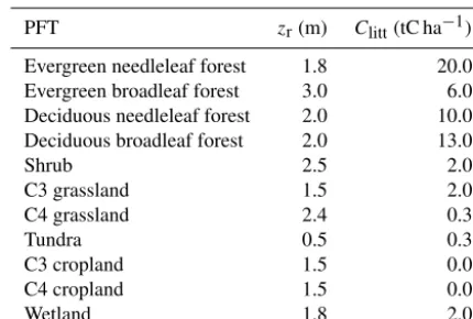
Table 1.CABLE parameter values for maximum rooting depth (zr) and above-ground fine structural litter (Clitt).
PFT zr(m) Clitt(tC ha−1)
Evergreen needleleaf forest 1.8 20.0
Evergreen broadleaf forest 3.0 6.0
Deciduous needleleaf forest 2.0 10.0
Deciduous broadleaf forest 2.0 13.0
Shrub 2.5 2.0
C3 grassland 1.5 2.0
C4 grassland 2.4 0.3
Tundra 0.5 0.3
C3 cropland 1.5 0.0
C4 cropland 1.5 0.0
Wetland 1.8 2.0
(Table 1) are set according to the depth at which the cumu-lative root fraction from the surface is 99 %, as estimated by Zeng (2001), using data from Canadell et al. (1996).
Note that while the functional form of Eq. (7) is taken from Lai and Katul (2000), there is not a direct equivalence of pa-rameter values because of its different implementation here. In particular, we use the root shut-down function to deter-mine stomatal drought response via Eq. (9), whereas Lai and Katul (2000) multiply it by a maximum efficiency function, which is in turn scaled by local root density and potential evaporation to obtain actual root water extraction.
Equations (6)–(9) are evaluated after each call to the sub-routine that solves the coupled equations for stomatal con-ductance, photosynthesis and leaf energy balance, which in-cludes the calculation of the transpiration rate. Since this subroutine is called four times within a loop in which at-mospheric stability is iteratively updated, updates tofw,soil
feed back to coupled transpiration and photosynthesis. In the extreme case where the initial transpiration estimate leads tofw,soil=0, the subsequently calculated transpiration and
photosynthesis are zero, and all net radiation absorbed by the leaf is converted to sensible heat. This is in contrast to the default model where photosynthesis may proceed in the ab-sence of extractable water.
2.2 Soil surface energy balance 2.2.1 Standard model
The latent heat flux,λEsoil(W m−2), and sensible heat flux,
Hsoil(W m−2) from the soil are calculated as follows:
λEsoil=min
cwλ1z1(θ1−θw) /1t, ws
0 Rnet,soil−G0
+(1−0)λρa q
∗
(Tsoil,1)−qc
rsoil
!# (10)
Hsoil=cpρa Tsoil,1−Ta/rsoil. (11)
The latent heat flux at the soil surface is the lesser of a sup-ply and demand term, where the demand term is calculated as the Penman–Monteith potential evaporation, scaled down by a soil wetness factor. In Eqs. (10) and (11),cwis the
den-sity of water (kg m−3),1z1is the thickness of the top soil
layer (m),wsis a soil wetness factor,λthe latent heat of
fu-sion (J kg−1),ρathe density of air (kg m−3), 0=s/ (s+γ ),
s is the slope of saturated vapour pressure with respect to temperature (m3(H2O) m−3(air) K−1),cp the heat capacity
of dry air (kg m−3K−1),γ=cp/λis the psychrometric
con-stant,q∗ is the saturated specific humidity (kg kg−1),qc is
in-canopy specific humidity (kg kg−1), andrsoil is the
resis-tance to turbulent transfer from the soil–air interface to the displacement height (s m−1). The soil wetness factor scales down the Penman–Monteith potential evaporation, and is cal-culated as
ws=min
1,θ1−0.5θw θfc−0.5θw
. (12)
Net radiation absorbed by the soil (Rnet,soil)is calculated
as the sum of shortwave and longwave components (Wang et al., 2011), where the longwave component depends on the surface soil temperature (assumed the temperature of the top soil layer) from the previous time step. The ground heat flux (G0)is calculated as the residual of the surface energy
bal-ance from the previous time step.
The resistancersoilis formulated as the integral over height
zof the inverse eddy diffusivity from the roughness length of the soil (z0s)to the displacement height in the canopy (d):
rsoil= d
Z
z0s dz σ2
wτL
, (13)
where the vertical velocity standard deviation (σw)is
formu-lated as
σw=u∗a3exp
n
cswL
z
h−1
o
, (14)
and the Lagrangian timescale as
τL=
c
T Lh
u∗
z
d, (15)
wherea3andcT Lare constants with respective values of 1.25
and 0.40;Lis leaf area index;u∗the friction velocity at the
top of the canopy; h the canopy height; andcsw is a
con-stant determining the rate of decrease ofσwwith depth in the
canopy, with value set to 1.0.
The default model uses an approximation to the integral in Eq. (13), which assumes a fixed value ofσwwith height over
the range of interest:
rsoil'
1
σ2 w
d
Z
z0s
1
τL
=ln d
z0s
exp{2c
swL} −exp
2cswL 1−dh
a23cT L2cswL
where
σ2
w=
1
d
d
Z
0
σw2dz, (17)
as used by Raupach et al. (1997) and subsequently propa-gated to CABLE (Wang et al., 2011, Eq. A.14). However, the analytic form of the integral(Haverd et al., 2013) is
rsoil=
1
u∗
ln d
z0s
exp2c
s,wL dh
a23cT L
, (18)
and results in higher values ofrsoil.
2.2.2 Leaf litter effects on surface energy balance Resistances to heat and water vapour transfer at the soil–air interface are augmented by a component representing the ef-fect of litter:
rbh=rsoil+
1zlitt
ρakH,litt
(19)
rbw=rsoil+
1zlitt
Dv,litt
, (20)
where1zlittis the depth of fine structural litter (m) andkH,litt
is the thermal conductivity of the litter layer. The depth of the litter layer is
1zlitt=
2.0Clitt
ρlitt
, (21)
where Clitt is the above-ground fine structural litter pool
(kg(C) m−2), inherited here on a PFT basis from the carbon-cycle component of the model, under the assumption that half the total fine structural litter (derived from leaf and root turnover) is stored aboveground. Values of Clitt are given
in Table 1. These were obtained by running the model for 18 FLUXNET sites (Table 2) with biogeochemistry enabled (carbon cycle only: nitrogen and phosphorous cycles were disabled) using repeated GSWP-2 3-hourly meteorology for the 1986–1995 period (Dirmeyer et al., 2006) until carbon pool convergence was achieved. Values ofClittused here are
internally consistent with the carbon-cycle-enabled version of CABLE. They do not reflect observation directly and were extrapolated to PFT-specific parameter values for the purpose of simulations (such as those presented here) which do not include the carbon cycle. However, for simulations with the carbon-cycle-enabled version, we recommend the use of in-ternal litter carbon pools instead.
The factor of 2.0 in Eq. (21) converts from mass of car-bon to mass of dry matter, and ρlitt is the bulk density of
litter, here 62 kg m−3(Matthews, 2005). Vapour diffusivity within the litter is estimated using the empirical formulation
of Matthews (2005):
DT(zlitt)=DT0exp
χ
z
litt
1zlitt −1
(22)
DT0=DT0,aexp U DT0,b (23)
χ=χa+U χb, (24)
wherezlittis the depth within the litter (set here to 0.51zlitt);
U is wind speed 10 cm above the litter surface; andχa,χb,
DT0,a, andDT0,bare empirical coefficients with respective
values of 2.08, 2.38 m−1s, 2×10⁻⁵m2s−1, and 2.60 m−1s. Heat conductivity of the litter layer is also taken from Matthews (2005):
kH,L=0.2+0.14θlitt
ρw
ρlitt
. (25)
Here,θlittis the volumetric moisture content of the litter. For
reasons of computational efficiency, and unlike Haverd and Cuntz (2010), we do not solve forθlitt, instead assuming a
fixed value of half of the saturated moisture content, here taken as 0.09 (Matthews, 2005).
2.2.3 SLI soil model Surface energy balance
The SLI (Soil-Litter-Iso) model (Haverd and Cuntz, 2010; Haverd et al., 2013) extends Ross’ fast numerical solution (Ross, 2003) of the Richards equation to include coupled ver-tical heat and moisture fluxes in the soil, including advective heat fluxes and stable isotopes of water (not used here). In contrast to the standard CABLE soil model, SLI solves for the coupled energy moisture fluxes at the air/soil interface:
Rnet,soil=
ρacp
rbh
(Tsurface−Tc)+λmin
Epot, Evap+Eliq
+ kH,1
1z12
Tsurface−Tsoil,1 (26)
The net radiation absorbed by the soil Rnet,soil (W m−2)
is calculated as in the standard CABLE2.0, except that we use the temperature at the soil–air interface (and not the tem-perature of the top soil layerTsoil,1)to represent the surface
temperatureTsurface. On the right-hand side of Eq. (26), the
first term is the sensible heat flux (Hsoil), withrbhthe
resis-tance to sensible heat transfer (s m−1). The third term is the conduction of heat into the soil, withkH,1the thermal
con-ductivity of the top soil layer (W m−1K−1). The second term is the latent heat of soil evaporation, withEpotthe soil
evap-oration at a surface relative humidity of 1; andEvapandEliq
(kg m−2s−1) from within the soil column to the surface:
Epot= (27)
ρacp DakH,1rbh+0.51z1ρacp
+rbhs(Tc)
0.51z1Rnet,soil+kth Tsoil,1−Tc
cp
λ
rbw kthrbh+0.51z1ρacp
+0.51z1rbhρacps(Tc)
Evap=
hr,1cv,sat(T1)−cv,a
rb,w+(1z1/2) /Dv,1
(28)
Eliq=ρw
φ
l(hr,1)−φmin
1z1/2
−K1
, (29)
where Da is the humidity deficit (m3(H2O) m−3(air)) in
the canopy; rb,w is the resistance to water vapour transfer
(s m−1);s is the slope of saturated vapour pressure with re-spect to temperature (m3(H2O) m−3(air) K−1);hr,1is the
rel-ative humidity in the top soil layer; cv,sat is the saturated
vapour concentration (m3(H2O) m−3(air));Dv,1is the vapour
diffusivity in the top soil layer (m2s−1);ϕlis the liquid
ma-tric flux potential (m2s−1); K1 is the hydraulic
conductiv-ity of the top soil layer (m s−1); and ϕmin (m2s−1) is the
matric flux potential corresponding to minimum soil mois-ture potential, set here tohmin=d−106m.Epotcomes from
the solution of the coupled energy and moisture conservation equations at the soil–air interface with relative humidity at the surface set to 1 (Haverd and Cuntz, 2010; Haverd et al., 2013).
Improved parameterization of in-canopy resistance to turbulent transfer
We adapt the CABLE2.0 formulation ofrsoil to account for
local (in-canopy) stability effects on the resistance of transfer from the ground to the canopy air space, effectively increas-ing the resistance when ground sensible heat fluxes are nega-tive. The adaptation splits the resistance into the sum of two components: the first isrsoil,afrom the soil roughness height
to a shear height zsh, and the second is rsoil,b from zsh to
the displacement heightd. We assume that the shear height, representing the depth of the shear-driven surface layer that forms along the ground surface under the canopy, is a small fraction of the canopy height, here 0.1. Both resistance com-ponents, like the originalrsoil,(Eq. 18) are integrals over the
inverse of the eddy diffusivityKf:
rsoil,a= zsh Z
z0s dz Kf(z)
(30)
rsoil,b= d
Z
zsh dz Kf(z)
, (31)
where alternate forms of the eddy diffusivity are specified: the first accounts for local stability effects, and the second is the same as in the original formulation ofrsoil:
Kf(z)=
κzue∗
8h
z
e L
z0s< z < zsh 1
σ2 wτL
zsh< z < d
. (32)
This yields
rsoil,a=ue∗
zsh R z0,s 8h z e L
κz dz
= e u∗ ln zsh z0s −ψh
zsh
e
L
+ψh
z0s e L , (33) and
rsoil,b=
1
u∗
ln d
zsh
exp 2c
s,wL(d/ h)
a32cT L
(34) In Eqs. (32)–(34),κ is the von Karman constant (0.4),8h
is the Monin–Obukhov stability function (Garratt, 1992), and e
u∗is the friction velocity at heightzshand is related to the
friction velocity at the reference height above the canopy by the same factor that attenuates the mean wind speed in the canopy:
e
u∗=u∗exp
n −cu
1−zsh
h
o
, (35)
wherecu is the exponent for an assumed exponential wind
profile (Raupach, 1994).eLis the local Obukhov length, cor-respondingly given by
e
L= −eu
3
κTg
K
Hsoil
ρacp
, (36)
wheregis the gravitational constant andTKis the canopy air
temperature (K).
3 Data
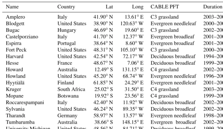
FLUXNET site locations, IGBP plant functional type, and data duration are listed in Table 2, combining information from Best et al. (2015) and De Kauwe et al. (2015a).
4 Simulations
For each site, CABLE2.0 was run using local half-hourly me-teorology from the flux tower. Model soil and vegetation pa-rameters were held fixed at their default values for the site PFT and CABLE’s 1◦×1◦ gridded soil texture. Leaf area index was prescribed using a 1◦×1◦gridded monthly cli-matology from the MODIS Collection 5 product (Ganguly et al., 2008). Model runs were initialized by repeated forc-ing with site data until soil moisture and temperature conver-gence were achieved.
For each site, four simulations, distinguished by model configuration were performed: (i) the standard CABLE2.0 model (STD); (ii) the standard CABLE2.0 model with the new drought response (STD_NDR); (iii) the standard CA-BLE2.0 with the new drought response and litter effect on soil evaporation (STD_NDR_LIT); and (iv) the standard CA-BLE2.0 with SLI hydrology, including the local stability cor-rection to the soil–canopy resistance (SLI). Note here that SLI already includes the new drought response and effects of litter on soil evaporation.
The new drought response parameterization requires a pa-rameter, γ, which appears in the root shut-down function (Eq. 7 ) and is related to drought tolerance. We selected a single global value ofγ=0.03, which gave the best model performance, as assessed against monthly latent heat obser-vations, over a range of values (0.01–0.12) for the SLI con-figuration.
5 Results and discussion
5.1 Evaluation against FLUXNET data
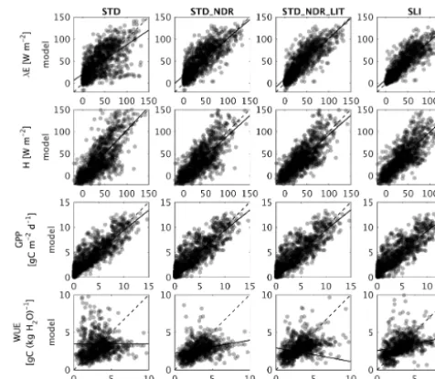
Figure 1 compares modelled monthly mean fluxes of latent heat flux (λE), sensible heat flux (H), GPP, and water use ef-ficiency (defined here as GPP divided by ET and filtered for observed monthly mean GPP>0.5 g C m−2d−1and monthly mean ET>0.00 kg(H2O) d−1)for the four model
configu-rations. Corresponding evaluation metrics are presented in Table 3. Figure 1 (STD) reveals clouds of points associ-ated with very low latent heat fluxes and very high water use efficiencies compared with observations. This problem is largely resolved by the new drought response formula-tion (STD_NDR). Correspondingly, root mean squared er-ror (RMSE) is reduced from 27 to 23 W m−2forλE, from 27 to 23 W m−2forH, and from 3.4 to 2.3 g(C) kg(H2O)−1
for WUE (Table 3). Model performance is further improved with the introduction of litter effects and SLI, particularly for evapotranspiration, with RMSE being further reduced from 23 to 17 W m−2 (Table 3). The improvement in H
Figure 1. Monthly modelled vs. observed latent heat, sensible heat, GPP, and total water use efficiency for four model configu-rations: (i) standard CABLE2.0 (STD); (ii) new drought response (STD_NDR); (iii) new drought response with litter effects on soil evaporation (STD_NDR_LIT); and (iv) full SLI. Solid lines: linear regression fits; dashed lines: 1 to 1. Darker shading indicates higher density of points.
is smaller, consistent with significant discrepancies between modelled and observed available energy (Rnet, not shown),
which are not expected to be resolved by the changes intro-duced here. Model performance for GPP is largely invari-ant across the four model configurations. All other metrics of Best et al. (2015) produced a consistent picture (onlyR2, shown in Table 2).
Table 2.List of FLUXNET site locations.
Name Country Lat Long CABLE PFT Duration
Amplero Italy 41.90◦N 13.61◦E C3 grassland 2003–2006
Blodgett United States 38.90◦N 120.63◦W Evergreen needleleaf 2000–2006
Bugac Hungary 46.69◦N 19.60◦E C3 grassland 2002–2006
Castelporziano Italy 41.70◦N 12.37◦W Evergreen broadleaf 2001–2006
Espirra Portugal 38.64◦N 8.60◦W Evergreen broadleaf 2001–2006
Fort Peck United States 48.31◦N 105.10◦W C3 grassland 2000–2006
Harvard United States 42.54◦N 72.17◦W Deciduous broadleaf 1994–2001
Hesse France 48.67◦N 7.06◦E Deciduous broadleaf 1999–2006
Howard Australia 12.49◦S 131.15◦E C4 grassland 2002–2005
Howland United States 45.20◦N 68.74◦W Evergreen needleleaf 1996–2004
Hyytiälä Finland 61.85◦N 24.29◦E Evergreen needleleaf 2001–2004
Kruger South Africa 25.02◦S 31.50◦E C4 grassland 2003–2004
Mopane Botswana 19.92◦S 23.56◦E C4 grassland 1999–2001
Roccarespampani Italy 42.40◦N 11.92◦W Deciduous broadleaf 2002–2006 Sylvania United States 46.24◦N 89.35◦W Deciduous broadleaf 2002–2005
Tharandt Germany 58.97◦N 13.57◦W Evergreen needleleaf 1998–2005
Tumbarumba Australia 38.66◦S 148.15◦E Evergreen broadleaf 2002–2005 University Michigan United States 48.56◦N 84.71◦W Deciduous broadleaf 1999–2003
Table 3.Evaluation metrics correlation coefficient (R2), root mean square error (RMSE), and bias error (BE) for monthly latent heat, sensible heat, GPP, and WUE predicted using four model configu-rations: (i) standard CABLE2.0 (STD); (ii) new drought response (STD_NDR); (iii) new drought response with litter effects on soil evaporation (STD_NDR_LIT); and (iv) full SLI.
STD STD_NDR STD_NDR_LIT SLI
R2 λE 0.41 0.65 0.72 0.74 H 0.58 0.60 0.63 0.63
GPP 0.76 0.74 0.74 0.74
WUE 0.00 0.06 0.09 0.08
RMSE λE 27.49 22.69 18.92 16.69 H 27.26 23.01 20.93 22.17
GPP 1.73 1.79 1.81 1.77
WUE 3.39 2.34 2.26 2.31
BE λE 7.7 11.2 6.8 3.8
H 0.05 −2.9 0.9 4.5
GPP 0.6 0.5 0.6 0.5
WUE 0.0 −0.7 −0.4 −0.2
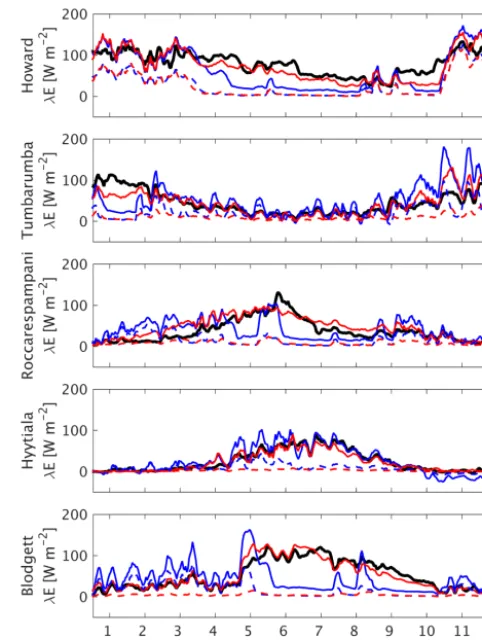
Roccarespampani: the STD model configuration predicts a severe decline inλEduring the 2003 drought episode, which is not seen in either the observations or the SLI configuration (Fig. 3). At Hyytiälä, litter effects improve simulations in the spring, while the improved modelling of in-canopy stability effects in SLI correct the highly negative winter latent heat fluxes produced by the other model configurations. Finally, at Blodgett, we see marked improvements due to the new drought response and litter effects: the STD model shows an unrealistic summer decline inλE, while the SLI config-uration tracks the observations well. Similar to Hyytiälä, the
STD configuration reveals an over-prediction ofλE at the start of the growing season. This is associated with exces-sive soil evaporation, not seen in the SLI simulations, largely because of leaf litter effects, with further dampening of soil evaporation in SLI by the modified resistance parameteriza-tions (Eqs. 33 and 34).
The significant effect of leaf litter on soil evaporation is anticipated. Ogée and Brunet (2002) and Gonzalez-Sosa et al. (1999, 2001) have demonstrated the importance of including litter on modelled soil evaporation in forest and agricultural ecosystems, respectively, while Haverd and Cuntz (2010) demonstrated that accounting for litter im-proved the timing and partitioning of latent heat fluxes at the Tumbarumba flux site.
Figure 2. Site-specific examples of monthly modelled vs. ob-served latent heat at five selected sites for four model configura-tions: (i) standard CABLE2.0 (STD); (ii) new drought response (STD_NDR); (iii) new drought response with litter effects on soil evaporation (STD_ NDR_LIT); and (iv) full SLI. Solid lines: linear regression fits; dashed lines: 1 to 1.
5.2 Sensitivity to drought tolerance parameter in the new drought response function
We explored a range of values (0.01–0.12) for the parame-terγ, which determines the steepness of the root shut-down function of Lai and Katul (2000) (Eq. 7), and is the sin-gle tunable parameter in the new drought response function (Eqs. 7–9).
Across the 18 FLUXNET sites, a value ofγ=0.03 gave the best results for the SLI model configuration, slightly higher than the low value of γ=0.01 (reflecting high drought tolerance) for Australian vegetation (Haverd et al., 2013). The optimum value varied from site to site but with no apparent relationship to aridity or plant functional type. For the present study, we therefore maintain a spatially in-variant value ofγ.
Further, the same was true when the data set was reduced to the drought-affected European sites (Tharandt, Hesse, Castelporziano, Roccarespampani, Espirra) during 2003, as selected by De Kauwe et al. (2015a). In this respect, our re-sults do not confirm the finding of De Kauwe et al. (2015a) that parameters representing high drought sensitivity at the most mesic sites and low drought sensitivity at the most
Figure 3.Illustrative 1-year (2003) time series of 14-day running mean modelled and observed latent heat at 5 selected sites, for two model configurations: (i) standard CABLE2.0 (STD) and (ii) full SLI. Modelled soil components are shown as well.
xeric sites are necessary to accurately model responses dur-ing drought.
may be much lower than suggested by the average profiles as-sumed in CABLE (e.g. Canadell et al., 1996), and root den-sity profiles are dynamic, adapting to resource availability (e.g. Haverd et al., 2016; Schymanski et al., 2009).
5.3 Alternative drought response mechanism
There is current discussion about the mechanism by which soil moisture deficit impacts plant productivity: via stom-atal conductance or via the photosynthetic apparatus, or both (e.g. Piayda et al., 2014; Zhou et al., 2013). In light of this we conducted an experiment using the SLI model configu-ration, modified such that the maximum rate of RuBisCO activity (Vcmax)and the potential rate of electron transport
(Jmax)were reduced by the drought response factor fw,soil,
while the drought response of stomatal conductance was dis-abled. Optimum results were obtained with the same value of γ=0.03, and corresponding model performance varied remarkably little compared with the drought response being applied to stomatal conductance (results not shown). This ex-periment was not conducted to inform the mechanistic de-bate, but rather to illustrate that our model improvements are robust to changes in parameterizations such as this.
6 Conclusions
We have presented formulations for improved plant drought response and soil surface energy balance in CABLE2.0. The equations presented here for root water extraction and stom-atal drought response are not uniquely valid formulations, al-though they are parsimonious (requiring a single parameter) and aid in producing skilful simulations of ET at globally distributed FLUXNET sites. What is particularly important about the model improvements presented here is that stom-atal drought response and root water extraction are properly coupled such that over-extraction cannot occur and coupling between photosynthesis and transpiration is maintained, thus avoiding implausible water use efficiencies produced by the standard CABLE2.0 model configuration. Such model im-provements can only be meaningfully tested against observa-tional estimates of total ET if soil evaporation is accurately modelled. We have shown that a physically accurate descrip-tion of soil evaporadescrip-tion available via the SLI soil model significantly enhances predictions of total ET compared to the standard soil model in CABLE, in which supply-limited evaporation is an empirical function of upper layer soil mois-ture (Eqs. 10–12), and tends to be over-estimated, particu-larly in the absence of litter effects. We have also shown that when the standard model configuration is adapted to include the new drought response and the effect of litter on soil evap-oration, it performs almost as well (at the monthly timescale) as when the full SLI model is implemented.
Future work will entail merging the improvements demon-strated here with the new hydrological parameterizations in
CABLE (Decker, 2015), and a new module for woody vege-tation demography and landscape heterogeneity mediated by disturbance (Haverd et al., 2014). Global simulations will be evaluated against gridded global estimates of ET, GPP, vege-tation cover, biomass, and soil carbon, as well as interannual variations in atmospheric CO2concentration. This will
pro-vide benchmarks for the use of CABLE in global offline ap-plications (e.g. attribution of terrestrial carbon sink), and is a necessary step towards assessing whether the modifications lead to improvements in simulated climate when CABLE is coupled to an Earth system model.
7 Code availability
The source code can be accessed after registration at https: //trac.nci.org.au/trac/cable. Simulations in this work used re-vision no. 3432.
Acknowledgements. This work used eddy covariance data acquired by the FLUXNET community and in particular by the following networks: AmeriFlux (U.S. Department of Energy, Biological and Environmental Research,Terrestrial Carbon Program (DE-FG02-04ER63917 and DE-FG02-04ER63911)), AfriFlux, CarboAfrica, CarboEuropeIP, CarboItaly, CarboMont, ChinaFlux, FLUXNET-Canada (supported by CFCAS, NSERC, BIOCAP, Environment Canada, and NRCan), GreenGrass, KoFlux, LBA, NECC, OzFlux, TCOSSiberia, and USCCC. We acknowledge the financial support to the eddy covariance data harmonization provided by CarboEu-ropeIP, FAO-GTOS-TCO, iLEAPS, Max Planck Institute for Bio-geochemistry, the National Science Foundation, Tuscia University, Université Laval and Environment Canada, and the U.S. Depart-ment of Energy, and the database developDepart-ment and technical sup-port from Berkeley Water Center, Lawrence Berkeley National Lab-oratory, Microsoft Research eScience, Oak Ridge National Labora-tory, University of California, Berkeley, and University of Virginia. Vanessa Haverd’s contribution was made possible by funding from the Australian Climate Change Science Program.
Edited by: G. A. Folberth
Reviewed by: E. Blyth, H. Zheng, and one anonymous referee
References
Ahlström, A., Raupach, M. R., Schurgers, G., Smith, B., Arneth, A., Jung, M., Reichstein, M., Canadell, J. G., Friedlingstein, P., Jain, A. K., Kato, E., Poulter, B., Sitch, S., Stocker, B. D., Viovy, N., Wang, Y. P., Wiltshire, A., Zaehle, S., and Zeng, N.: The domi-nant role of semi-arid ecosystems in the trend and variability of the land CO2sink, Science, 348, 895–899, 2015.
Canadell, J., Jackson, R. B., Ehleringer, J. B., Mooney, H. A., Sala, O. E., and Schulze, E. D.: Maximum rooting depth of vegetation types at the global scale, Oecologia, 108, 583–595, 1996. Ciais, P., Sabine, C., Bala, G., Bopp, L., Brovkin, V., Canadell, J.,
Chhabra, A., DeFries, R., Galloway, J., Heimann, M., Jones, C., Le Quéré, C., Myneni, R. B., Piao, S., and Thornton, P.: Carbon and Other Biogeochemical Cycles, in: Climate Change 2013: The Physical Science Basis. Contribution of Working Group I to the Fifth Assessment Report of the Intergovernmental Panel on Climate Change Cambridge University Press, Cambridge, United Kingdom and New York, NY, USA, 2013.
Decker, M.: Development and evaluation of a new soil moisture and runoff parameterization for the CABLE LSM including subgrid-scale processes, J. Adv. Model. Earth Syst., 7, 1788–1809, 2015. De Kauwe, M. G., Zhou, S.-X., Medlyn, B. E., Pitman, A. J., Wang, Y.-P., Duursma, R. A., and Prentice, I. C.: Do land surface models need to include differential plant species responses to drought? Examining model predictions across a mesic-xeric gradient in Europe, Biogeosciences, 12, 7503–7518, doi:10.5194/bg-12-7503-2015, 2015a.
De Kauwe, M. G., Kala, J., Lin, Y.-S., Pitman, A. J., Medlyn, B. E., Duursma, R. A., Abramowitz, G., Wang, Y.-P., and Miralles, D. G.: A test of an optimal stomatal conductance scheme within the CABLE land surface model, Geosci. Model Dev., 8, 431–452, doi:10.5194/gmd-8-431-2015, 2015b.
Dirmeyer, P. A., Gao, X. A., Zhao, M., Guo, Z. C., Oki, T. K., and Hanasaki, N.: GSWP-2 – Multimodel anlysis and implications for our perception of the land surface, B. Am. Meteorol. Soc., 87, 1381–1397, 2006.
Ganguly, S., Samanta, A., Schull, M. A., Shabanov, N. V., Milesi, C., Nemani, R. R., Knyazikhin, Y., and Myneni, R. B.: Gener-ating vegetation leaf area index Earth system data record from multiple sensors. Part 2: Implementation, analysis and validation, Remote Sens. Environ., 112, 4318–4332, 2008.
Gardner, W. R.: dynamic aspects of water availability to plants, Soil Sci., 89, 63–73, 1960.
Garratt, J. R.: The Atmospheric Boundary Layer, Cambridge Uni-versity Press, 1992.
Gonzalez-sosa, E., Braud, I., Jean-Louis, T., Michel, V., Pierre, B., and Jean-Christophe, C.: Modelling heat and water exchanges of fallow land covered with plant-residue mulch, Agr. Forest Mete-orol., 97, 151–169, 1999.
Gonzalez-Sosa, E., Braud, I., Thony, J. L., Vauclin, M., and Calvet, J. C.: Heat and water exchanges of fallow land covered with a plant-residue mulch layer: a modelling study using the three year MUREX data set, J. Hydrol., 244, 119–136, 2001.
Haverd, V. and Cuntz, M.: Soil–Litter–Iso: A one-dimensional model for coupled transport of heat, water and stable isotopes in soil with a litter layer and root extraction, J. Hydrol., 388, 438– 455, 2010.
Haverd, V., Raupach, M. R., Briggs, P. R., Canadell, J. G., Isaac, P., Pickett-Heaps, C., Roxburgh, S. H., van Gorsel, E., Viscarra Rossel, R. A., and Wang, Z.: Multiple observation types reduce uncertainty in Australia’s terrestrial carbon and water cycles, Biogeosciences, 10, 2011–2040, doi:10.5194/bg-10-2011-2013, 2013.
Haverd, V., Smith, B., Nieradzik, L. P., and Briggs, P. R.: A stand-alone tree demography and landscape structure module for Earth system models: integration with inventory data from
temperate and boreal forests, Biogeosciences, 11, 4039–4055, doi:10.5194/bg-11-4039-2014, 2014.
Haverd, V., Smith, B., Raupach, M., Briggs, P., Nieradzik, L., Beringer, J., Hutley, L., Trudinger, C. M., and Cleverly, J.: Cou-pling carbon allocation with leaf and root phenology predicts tree–grass partitioning along a savanna rainfall gradient, Biogeo-sciences, 13, 761–779, doi:10.5194/bg-13-761-2016, 2016. Jackson, R. B., Canadell, J., Ehleringer, J. R., Mooney, H. A., Sala,
O. E., and Schulze, E. D.: A global analysis of root distributions for terrestrial biomes, Oecologia, 108, 389–411, 1996.
Jung, M., Vetter, M., Herold, M., Churkina, G., Reichstein, M., Za-ehle, S., Ciais, P., Viovy, N., Bondeau, A., and Chen, Y.: Uncer-tainties of modeling gross primary productivity over Europe: A systematic study on the effects of using different drivers and ter-restrial biosphere models, Global Biogeochem. Cy., 21, GB4021, doi:10.1029/2006GB002915, 2007.
Kala, J., De Kauwe, M. G., Pitman, A. J., Lorenz, R., Medlyn, B. E., Wang, Y.-P., Lin, Y.-S., and Abramowitz, G.: Implementa-tion of an optimal stomatal conductance scheme in the Australian Community Climate Earth Systems Simulator (ACCESS1.3b), Geosci. Model Dev., 8, 3877–3889, doi:10.5194/gmd-8-3877-2015, 2015.
Kala, J., De Kauwe, M. G., Pitman, A. J., Medlyn, B. E., Wang, Y.-P., Lorenz, R., and Perkins-Kirkpatrick, S. E.: Impact of the representation of stomatal conductance on model projections of heatwave intensity, Scientific Reports, 6, 2016.
Kowalczyk, E., Stevens, L., Law, R., Dix, M., Wang, Y., Harman, I., Haynes, K., Srbinovsky, J., Pak, B., and Ziehn, T.: The land surface model component of ACCESS: description and impact on the simulated surface climatology, Aust. Meteorol. Oceanogr. J., 63, 65–82, 2013.
Lai, C.-T. and Katul, G.: The dynamic role of root-water uptake in coupling potential to actual transpiration, Adv. Water Resour., 23, 427–439, 2000.
Law, R. M., Ziehn, T., Matear, R. J., Lenton, A., Chamberlain, M. A., Stevens, L. E., Wang, Y. P., Srbinovsky, J., Bi, D., Yan, H., and Vohralik, P. F.: The carbon cycle in the Australian Commu-nity Climate and Earth System Simulator (ACCESS-ESM1) – Part 1: Model description and pre-industrial simulation, Geosci. Model Dev. Discuss., 8, 8063–8116, doi:10.5194/gmdd-8-8063-2015, 2015.
Li, L., Wang, Y.-P., Yu, Q., Pak, B., Eamus, D., Yan, J., van Gorsel, E., and Baker, I. T.: Improving the responses of the Australian community land surface model (CABLE) to seasonal drought, J. Geophys. Res.-Biogeo., 117, G04002, doi:10.1029/2012JG002038, 2012.
Lorenz, R., Pitman, A. J., Donat, M. G., Hirsch, A. L., Kala, J., Kowalczyk, E. A., Law, R. M., and Srbinovsky, J.: Represen-tation of climate extreme indices in the ACCESS1.3b coupled atmosphere–land surface model, Geosci. Model Dev., 7, 545– 567, doi:10.5194/gmd-7-545-2014, 2014.
Matthews, S.: The water vapour conductance of Eucalyptus litter layers, Agr. Forest Meteorol., 135, 73–81, 2005.
Ogée, J. and Brunet, Y.: A forest floor model for heat and moisture including a litter layer, J. Hydrol., 255, 212–233, 2002. Oleson, K. W., Niu, G. Y., Yang, Z. L., Lawrence, D. M., Thornton,
Geo-phys. Res.-Biogeo., 113, G01021, doi:10.1029/2007JG000563, 2008.
Piao, S., Sitch, S., Ciais, P., Friedlingstein, P., Peylin, P., Wang, X., Ahlström, A., Anav, A., Canadell, J. G., Cong, N., Huntingford, C., Jung, M., Levis, S., Levy, P. E., Li, J., Lin, X., Lomas, M. R., Lu, M., Luo, Y., Ma, Y., Myneni, R. B., Poulter, B., Sun, Z., Wang, T., Viovy, N., Zaehle, S., and Zeng, N.: Evaluation of terrestrial carbon cycle models for their response to climate vari-ability and to CO2trends, Glob. Change Biol., 19, 2117–2132, 2013.
Piayda, A., Dubbert, M., Rebmann, C., Kolle, O., Costa e Silva, F., Correia, A., Pereira, J. S., Werner, C., and Cuntz, M.: Drought impact on carbon and water cycling in a MediterraneanQuercus suberL. woodland during the extreme drought event in 2012, Biogeosciences, 11, 7159–7178, doi:10.5194/bg-11-7159-2014, 2014.
Raupach, M.: Simplified expressions for vegetation roughness length and zero-plane displacement as functions of canopy height and area index, Bound.-Lay. Meteorol., 71, 211–216, 1994. Raupach, M. R.: Dynamics and optimality in coupled terrestrial
en-ergy, water, carbon and nutrient cycles, in: Predictions in un-gauged basins: international perspectives on the state of the art and pathways forward, edited by: Franks, S. W. S., Takeuchi, K., and Tachikawa, Y., International Association of Hydrologi-cal Sciences 2005, 2005.
Raupach, M. R., Finkele, K., and Zhang, L.: SCAM (Soil-Canopy Atmosphere Model): Description and comparison with field data, CSIRO Centre for Environmental Mechanics, Canberra, ACT, Australia, 1997.
Ross, P. J.: Modeling soil water and solute transport – Fast, simpli-fied numerical solutions, Agron. J., 95, 1352–1361, 2003. Ryel, R., Caldwell, M., Yoder, C., Or, D., and Leffler, A.: Hydraulic
redistribution in a stand of Artemisia tridentata: evaluation of benefits to transpiration assessed with a simulation model, Oe-cologia, 130, 173–184, 2002.
Sakaguchi, K. and Zeng, X.: Effects of soil wetness, plant litter, and under-canopy atmospheric stability on ground evaporation in the Community Land Model (CLM3.5), J. Geophys. Res.-Atmos., 114, D01107, doi:10.1029/2008jd010834, 2009.
Schymanski, S. J., Sivapalan, M., Roderick, M. L., Hutley, L. B., and Beringer, J.: An optimality-based model of the dynamic feedbacks between natural vegetation and the water balance, Water Resour. Res., 45, W01412, doi:10.1029/2008wr006841, 2009.
Sitch, S., Friedlingstein, P., Gruber, N., Jones, S. D., Murray-Tortarolo, G., Ahlström, A., Doney, S. C., Graven, H., Heinze, C., Huntingford, C., Levis, S., Levy, P. E., Lomas, M., Poul-ter, B., Viovy, N., Zaehle, S., Zeng, N., Arneth, A., Bonan, G., Bopp, L., Canadell, J. G., Chevallier, F., Ciais, P., Ellis, R., Gloor, M., Peylin, P., Piao, S. L., Le Quéré, C., Smith, B., Zhu, Z., and Myneni, R.: Recent trends and drivers of regional sources and sinks of carbon dioxide, Biogeosciences, 12, 653– 679, doi:10.5194/bg-12-653-2015, 2015.
Wang, Y.-P. and Leuning, R.: A two-leaf model for canopy con-ductance, photosynthesis and partitioning of available energy I:: Model description and comparison with a multi-layered model, Agr. Forest Meteorol., 91, 89–111, 1998.
Wang, Y. P., Law, R. M., and Pak, B.: A global model of carbon, nitrogen and phosphorus cycles for the terrestrial biosphere, Bio-geosciences, 7, 2261–2282, doi:10.5194/bg-7-2261-2010, 2010. Wang, Y. P., Kowalczyk, E., Leuning, R., Abramowitz, G., Rau-pach, M. R., Pak, B., van Gorsel, E., and Luhar, A.: Di-agnosing errors in a land surface model (CABLE) in the time and frequency domains, J. Geophys. Res., 116, G01034, doi:10.1029/2010JG001385, 2011.
Zeng, X.: Global Vegetation Root Distribution for Land Modeling, J. Hydrometeorol., 2, 525–530, 2001.
Zhang, H., Pak, B., Wang, Y. P., Zhou, X., Zhang, Y., and Zhang, L.: Evaluating Surface Water Cycle Simulated by the Australian Community Land Surface Model (CABLE) across Different Spa-tial and Temporal Domains, J. Hydrometeorol., 14, 1119–1138, 2013.
Zhou, S., Duursma, R. A., Medlyn, B. E., Kelly, J. W., and Pren-tice, I. C.: How should we model plant responses to drought? An analysis of stomatal and non-stomatal responses to water stress, Agr. Forest Meteorol., 182, 204–214, 2013.