R E S E A R C H
Open Access
A solution with cubic boundary elements for
the compressible fluid flow around obstacles
Lumini¸ta Grecu
**Correspondence: [email protected] Department of Applied
Mathematics, University of Craiova, Craiova, Romania
Abstract
The paper presents a solution of the problem of the 2D compressible fluid flow around obstacles, based on the boundary element method in which the singular boundary integral equation is solved with cubic boundary elements. In this approach the singular boundary integral with sources distribution is considered. The numerical method is implemented into a computer code developed under Mathcad, and numerical solutions for some particular cases are obtained. Numerical solutions are compared with analytical ones for cases when the latter exist. A good agreement between them can be observed even when the number of nodes chosen for the boundary discretization is quite small, the fact that shows the great efficiency of the exposed method.
MSC: 65N38; 76M15; 76G25; 35Q35
Keywords: boundary element method; cubic boundary element; singular boundary
integral equation; compressible fluid flow
1 Introduction
Many of the phenomena studied in the nature are described by boundary value problems, in fact, by partial differential equations or systems of partial differential equations with boundary restrictions, and only few of them can be, in general, solved analytically.
One powerful numerical technique that can be used to solve such problems is the boundary element method. This method has been widely used to solve partial differen-tial equations or systems of pardifferen-tial differendifferen-tial equations with boundary conditions, many books being dedicated to this subject (for example, [–]).
The boundary element method consists in solving, by discretization, a boundary integral equation, equivalent to the mathematical model of the problem to solve, by using finite elements named boundary elements. When applying this method, two big steps have to be done: first a boundary integral formulation is obtained, and usually it represents a singular boundary integral equation or a system of singular boundary integral equations, and then this singular integral equation is solved and numerical solutions are found.
When the problem to solve is described by systems of partial differential equations with fundamental solutions, this method can be successfully applied even if the boundary con-ditions are not linear, as in the case of the problem considered in this paper. The method is suitable for problems with infinite domains, as those of fluid flows around obstacles, because the fundamental solutions satisfy conditions that do not involve the presence of a fictive boundary at great distance. Other numerical methods such as finite difference
method, finite volume method and finite element method can be applied to solve prob-lems of fluid flow (see, for example, []), but the obstacle needs to be placed in a grid, and so the computational effort is quite big. The boundary element method has another great advantage over these, because it reduces the dimension of the problem by one and also the necessary computational effort.
In this paper, based on this method, a numerical solution for the two-dimensional prob-lem of the compressible fluid flow around obstacles is obtained. The probprob-lem of the fluid flow around obstacles has been the subject of many papers, among which we mention [–], some of them dealing only with the incompressible case. The boundary element method has also been applied to solve this problem, but in this approach, a singular bound-ary integral equation formulated in velocity terms is considered, and the solution is eval-uated by using higher-order boundary elements. So, the primary variables of interest are directly numerically evaluated without needing a differentiation process, as in the case of other approaches in which the stream function or the potential of the fluid flow are envisaged.
This paper is focused on the second step in applying this method, namely on solving the singular boundary equation which arises when at the first step an indirect technique with sources distribution is considered.
Briefly, the problem to solve is that of a subsonic uniform compressible fluid flow per-turbed by the presence of an obstacle of boundaryCassumed to be smooth and closed. The goal is to find out the perturbation produced by the obstacle and the fluid action on it. The mathematical model of the problem consists in a system of partial differential equa-tions with a nonlinear boundary condition. In dimensionless variables, it can be written as (see [], chap. )
⎧ ⎨ ⎩
∂u ∂x+
∂v ∂y= , ∂v
∂x– ∂u ∂y= ,
(β+u)nx+βvny= onC,
lim(u,v) = ∞ (perturbation vanishes at great distances),
()
where u
β andvare the components of the perturbation velocity,nx,nydenote the com-ponents of the normal unit vector outward the fluid,β=√ –M(for the subsonic flow),
andM= Mach number.
Assimilating the boundary with a continuous distribution of sources, of intensityf, and assuming that f satisfies a Hölder condition onC, in [], chap. , a singular boundary integral equation is deduced. It has the following expression:
nx+βnyf(x¯) +
π
C
f(x¯)(x–x)n
x+β(y–y)ny
¯x–x¯
ds= βnx, ()
wheren
x,ny denote the components of the normal unit vector outward the fluid in the pointx¯∈C. The sign ‘’ denotes the Cauchy principal value of the integral.
Using cubic boundary elements to solve this singular boundary integral equation, we obtain a better approximation for the solution, because cubic boundary elements offer a better approximation not only for the unknown of the problem, but also for the geometry of the boundary involved.
Using the approximation models, the problem is reduced to a linear system of equa-tions, which has as unknowns the nodal values of the sources intensities. After solving it, the components of the perturbation velocities and the local pressure coefficient are nu-merically evaluated.
A difficult stage in solving singular boundary integral equations is the treatment of the singularities that arise. Different methods can be applied to overpass this difficulty (see, for example, [, ]). Numerical evaluation of integrals of singular kernels is a very im-portant aspect for a well-conditioned behavior of the system matrix. In paper [] a regu-larization technique with modified shape functions has been applied. In this approach, the coefficients arising from integrals of singular kernels are evaluated with a simple method, namely the truncation method.
2 The discretized equation
In the herein boundary element approach for solving the singular boundary integral equa-tion (), the boundary is divided intoNcubic boundary elements, notedLj,j= ,N. Each cubic boundary element has four nodes: two extremes and two interior ones. Nnodes are used for the boundary discretization, because each boundary element has two common nodes with the two adjacent boundary elements.
So, we obtain the discretized form of equation ():
nx+βnyf(x¯) +
π
N
j=
Lj
f(x¯)(x–x)n
x+β(y–y)ny
¯x–x¯
ds= βnx. ()
Considering that the discretized equation is satisfied in every nodex¯i, and denoting by
Ai=nix
+βni y
, we get the following equation, in fact, we get Nequations - the linear system the problem is reduced at
Aif(x¯i) +
π
N
j=
Lj
f(x¯)(x–xi)n i
x+β(y–yi)niy
¯x–x¯i
ds= βni
x, i= , N. ()
We further do not use the notation referring to the Cauchy principal value of an integral, but we take into account that whenx¯i∈Ljthe integrals in () have singular kernels, and
they are understood in this way, and whenx¯i∈/Ljthey are the usual ones.
From the family of cubic boundary elements, we choose the isoparametric ones. The cubic isoparametric boundary element uses the same set of basic functions (see [, ]), notedN,N,N,N, for describing the geometry and the unknown function. If the
ho-mogeneous variableξ is used, these functions have the following expressions, similar to those given in [], pp.-:
N(ξ) = –
(ξ– )(ξ+)(ξ–)
, N(ξ) =
(ξ+ )(ξ– )(ξ–)
,
()
N(ξ) = –
(ξ+ )(ξ– )(ξ+)
, N(ξ) =
(ξ+)(ξ–)(ξ+ )
For such a cubic boundary elementLj, the following approximation models stand:
x= [N] xj, y= [N] yj, f = [N] fj, () where [N] = (NNNN) is a line matrix,{xj},{yj},{fj}are the column matrices made with
the global coordinates ofLjnodes, and the nodal values of the unknown function corre-sponding to the same boundary element. Two systems of numbering are used: a global one (fj,j= , Nrepresents the nodal value corresponding to node numberj) and a local one (flj,l= , ,j= ,Nrepresents the nodal value of thelth node of element numberj).
We introduce in equation () the approximation models (), and we obtain
Aif(x¯i) +
π
N
j=
–
([N]{xj}–xi)nix
([N]{¯xj}–x¯
i)
[N] fjJj(ξ)dξ
+
π
N
j=
–
β([N]{yj}–yi)niy
([N]{¯xj}–x¯
i)
[N] fjJj(ξ)dξ= βnix, ()
where we denote byJj(ξ) the Jacobian coordinate transformation. We can write () as
Aif(x¯i) +
π
N
j=
–
Pji(ξ)ni x+βQ
j i(ξ) Rij(ξ) [N] f
jJj(ξ)dξ= βni
x, ()
where
Pji(ξ) = [N] xj–xi, Qji(ξ) = [N] yj–yi and Rij(ξ) =¯x–x¯i=[N] x¯j
–x¯i.
()
Further, we get
Aifi+
π
N
j=
l=
alijflj
= βnix, ()
where
alij=
–
Nln i xP
j
i(ξ) +βniyQ j i(ξ) Rij(ξ) J
j(ξ)dξ, i= , N,j= ,N,l= , . ()
Returning to the global system of numbering, we obtain the following linear algebraic system:
A{f}={B}, A∈MN(R),{f},{B} ∈RN, Bi= πβnix. ()
3 Coefficients evaluation
of them are usual integrals, and we can use any mathematical software to compute them, but the others are integrals of singular kernels. For the evaluation of the singular integrals, we use in this paper the truncation method, the method that brings good results when the integrand does not oscillate near the singularity (see [], chap. ), as in the following case.
Replacing relations () and () in (), then doing some calculus and notations, we get the expressions for the functions in (). For example, forPji(ξ) = [N]{xj}–xi, we get
Pji(ξ) =N(ξ)xj+N(ξ)xj+N(ξ)xj+N(ξ)xj–xi
=– (ξ– )
ξ+
ξ–
xj+
(ξ+ )(ξ– )
ξ–
xj
–
(ξ+ )(ξ– )
ξ+
xj+
ξ–
ξ–
(ξ+ )xj–xi
= – (ξ+ )
ξ–
xj+
ξ– ξ–
xj
–
ξ+
ξ– xj+ (ξ+ )
ξ–
xj–xi
=ajξ+ajξ+ajξ+aji,
where
aj=–x j
+ x
j
– x
j
+ x
j
, a
j
=
xj– xj– xj+ xj
,
aj=x j
– x
j
+ x
j
–x
j
, a
j
i=
–xj+ xj+ xj–xj
–xi.
Doing the same forQji,RijandJj, the following relations hold:
Qji(ξ) =bjξ+bjξ+bjξ+bji,
Rij(ξ) =rijξ+rijξ+rijξ+rijξ+rijξ+rijξ+rij,
Jj(ξ) =
gjξ+gj ξ+g
j
ξ+g
j
ξ+g
j
,
()
where
bj=–y j
+ y
j
– y
j
+ y
j
, b
j
=
yj– yj– yj+ yj
,
bj=y j
– y
j
+ y
j
–y
j
, b
j
i=
–yj+ yj+ yj–yj
–yi,
rij=aj+bj, rij= ajaj+bjbj, rij=aj+ ajaj+bj+ bjbj, rij= ajaji+ajaj+bjbji+bjbj, rij=aj+ajaji+bj+bjbji, () rij= ajaji+bjbji, rij=aji+bji, gj= aj+bj,
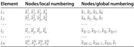
Table 1 Relation between the local and the global system of numbering
Element Nodes/local numbering Nodes/global numbering
L1 x¯11,x¯21,x¯31,x¯41 x¯1,¯x2,x¯3,x¯4 L2 x¯12,x¯22,x¯32,x¯42 x¯4,¯x5,x¯6,x¯7
· · · ·
Lj x¯1j,x¯ j 2,¯x
j 3,x¯
j
4 x¯3j–2,¯x3j–1,x¯3j,¯x3j+1
· · · ·
LN x¯1N,x¯2N,¯xN3,x¯N4 x¯3N–2,x¯3N–1,x¯3N,x¯1
The above relations allow us to evaluate the coefficients given by relation () with a computer code, because their expressions depend only on the nodes coordinates. In order to find the expressions of coefficients arising from integrals considered in a Cauchy prin-cipal value sense, for which we apply the truncation technique, we need to mention the connection between the two systems of numbering used in this approach: the global and the local one. This also has to be done for simplifying the implementation of the method exposed into a computer code.
Table shows the relations between the two systems of numbering.
For thejth boundary elementLj,j= ,N, the nodes have, in the global system of num-bering, the numbers j– , j– , j, j+ , understanding that node number N+ is node number , the boundary being closed. So, the coefficients given by relations () come from singular integrals only whenitakes one of the above valuesi∈ {j– , j– , j, j+ }; oth-erwise they come from the usual ones.
Using relations () and (), we have, ifi∈ {/ j– , j– , j, j+ }, the following expres-sions for the nonsingular coefficients given by ():
aij=
–
–ξ+ ξ+ξ–
·
nixPij(ξ) +βniyQji(ξ) Rij(ξ)
Jj(ξ)dξ, ()
aij=
–
(ξ–ξ– ξ+ )
·
ni xP
j
i(ξ) +βniyQ j i(ξ) Rij(ξ) J
j(ξ)dξ, ()
aij=
–
–(ξ+ξ– ξ– )
·
ni xP
j
i(ξ) +βniyQ j i(ξ) Rij(ξ) J
j(ξ)dξ, ()
aij=
–
ξ+ ξ–ξ–
·
ni xP
j
i(ξ) +βniyQ j i(ξ) Rij(ξ) J
j(ξ)dξ, i= , N,j= ,N. ()
In order to use the truncation method for evaluating the singular coefficients, we con-sider a very small parametereps> to reduce the domain of integration by eliminating the singularity. Taking into account the cases when the singularity arises, we get the following four situations.
. Wheni= j– , the singularity arises whenξ= –. The coefficients have in this case the expressions
alij=
–+eps
Nln i xP
j
i(ξ) +βniyQ j i(ξ) Rij(ξ)
. Wheni= j– , the singularity arises whenξ= –. The coefficients are in this case given by
alij=
––eps
–
Nln i xP
j
i(ξ) +βniyQ j i(ξ) Rij(ξ)
Jj(ξ)dξ
+
–+eps
Nln i xP
j
i(ξ) +βniyQ j i(ξ) Rij(ξ) J
j(ξ)dξ, l= , . ()
. Wheni= j, the singularity arises whenξ=. The coefficients are
alij=
–eps
–
Nln i xP
j
i(ξ) +βniyQ j i(ξ) Rij(ξ)
Jj(ξ)dξ
+
+eps
Nln i xP
j
i(ξ) +βniyQ j i(ξ) Rij(ξ) J
j(ξ)dξ, l= , . ()
. Finally, wheni= j+ , the singularity arises whenξ= , and so we have
alij=
–eps – Nln i xP j
i(ξ) +βniyQ j i(ξ) Rij(ξ)
Jj(ξ)dξ. ()
In order to obtain matrixAfrom relation (), we return to the global system of num-bering, and we write system () as follows:
πAifi+ N
j=
(Aij–fj–+Aij–fj–+Aijfj) = πβnix,
and further
πAifi+
N
k=
Aikfk= πβnix,
where
Aik=
⎧ ⎪ ⎪ ⎪ ⎪ ⎪ ⎨ ⎪ ⎪ ⎪ ⎪ ⎪ ⎩
aij+aij–, ifk= j– ,k= ,N, a
i+aiN, ifk= , a
ij, ifk= j– ,j= ,N, aj, ifk= j,j= ,N
⇔ Aik=
⎧ ⎪ ⎪ ⎪ ⎪ ⎪ ⎪ ⎪ ⎨ ⎪ ⎪ ⎪ ⎪ ⎪ ⎪ ⎪ ⎩ a
ik+ +a
ik– , ifk≡(mod),k= , N, ai+aiN, ifk= ,
a
ik+
, ifk≡(mod),k= , N,
a
k, ifk≡(mod),k= , N.
Finally, the system to solve is
N
k=
AAikfk=Bi, i= , N, Bi= πβnix, i= , N ()
with
AAik=
⎧ ⎨ ⎩
Aik, i=k,
πAi+Aii, i=k. ()
Solving system (), we find the nodal valuesf,f, . . . ,fN, and then we can evaluate the velocity components.
Under the same assumption, thatf satisfies a Hölder condition on the boundary, the components of the perturbation velocity can be obtained. On the boundary,u,vhave the following expressions (see [], chap. ):
u(x¯) = –
f(x¯)n
x– π C
f(x)¯ x–x
¯x–x¯
ds,
v(x¯) = –
f(x¯)n
y– π C
f(x)¯ y–y
¯x–x¯
ds.
()
Analogously, as in case of solving the boundary integral equation, we get the nodal ex-pressions of the velocity components. After the boundary discretization, after introduc-ing the approximation models () in the above relations, and after considerintroduc-ingx¯=xi,¯
i= , N, and doing some calculus, we obtain
u(xi) = –¯ fin i x– π N j= l=
blijflj
,
v(xi) = –¯ fin i y– π N j= l=
clijflj
, i= , N.
()
Using the same notations as before, we have:
blij=
–
Nl· P j i(ξ) Rij(ξ)
Jj(ξ)dξ,
clij=
–
Nl· Qji(ξ) Rij(ξ)J
j(ξ)dξ, l= , ,i= , N,j= ,N
()
and further, the following relations:
bij=
–
–ξ+ ξ+ξ–
·
Pji(ξ) Rij(ξ)
Jj(ξ)dξ,
bij=
–
(ξ–ξ– ξ+ )
·
Pji(ξ) Rij(ξ)J
j(ξ)dξ,
bij=
–
–(ξ+ξ– ξ– )
·
Pji(ξ) Rij(ξ)J
j(ξ)dξ,
bij=
–
ξ+ ξ–ξ–
·
Pij(ξ) Rij(ξ)J
j(ξ)dξ, i= , N,j= ,N,
cij=
–
–ξ+ ξ+ξ–
·
Qji(ξ) Rij(ξ)
Jj(ξ)dξ,
cij=
–
(ξ–ξ– ξ+ )
·
Qji(ξ) Rij(ξ)J
j(ξ)dξ,
cij=
–
–(ξ+ξ– ξ– )
·
Qji(ξ) Rij(ξ)J
j(ξ)dξ,
cij=
–
ξ+ ξ–ξ–
·
Qji(ξ) Rij(ξ)J
j(ξ)dξ, i= , N,j= ,N.
()
The coefficients from the above relations are evaluated in the same manner as in the case of the matrix coefficients; analogous formulas with ()-() stand in the case of singular integrals from () and ().
Finally, the following expressions for the velocity field components on the boundary are deduced from () using the connection between the two systems of numbering, and returning to the global one:
u(xi) =¯
N
k=
uikfk, v(xi) =¯
N k= vikfk, () where uik= ⎧ ⎨ ⎩
–nxi–πbbii, ifi=k,
–πbbik, ifi=k, vik=
⎧ ⎨ ⎩
–nyi–πccii, ifi=k,
–πccik, ifi=k, ()
bbik= ⎧ ⎪ ⎪ ⎪ ⎪ ⎪ ⎪ ⎪ ⎨ ⎪ ⎪ ⎪ ⎪ ⎪ ⎪ ⎪ ⎩ b
ik+ +b
ik– , ifk≡(mod),k= , N, bi+biN, ifk= ,
b
ik+
, ifk≡(mod),k= , N,
b
ik, ifk≡(mod),k= , N,
ccik=
⎧ ⎪ ⎪ ⎪ ⎪ ⎪ ⎪ ⎪ ⎨ ⎪ ⎪ ⎪ ⎪ ⎪ ⎪ ⎪ ⎩ c
ik+
+c
ik–
, ifk≡(mod),k= , N,
c
i+ciN, ifk= , c
ik+ , ifk≡(mod),k= , N, c
ik
, ifk≡(mod),k= , N.
()
Replacing relations () in () and then in (), we evaluate the nodal values of the com-ponents of velocity and then the local pressure coefficient with the following expression (whenM= ):
cp=
γM
+M
(γ– )
–v–
+u
β
γγ–
–
, ()
4 Numerical results and conclusions
Using a good method for evaluating the singular integrals that appear is a stage of great practical importance, because the coefficients given by these singular integrals are dom-inants situated near the diagonal of the matrix, and so they play an important role in es-tablishing a good behavior of the system.
The existence of particular cases for which the considered problem has an exact solution is of major significance because it allows us to test the developed method. In this paper we compare the numerical solution with the exact one in order to make an analytical checking of the exposed method. The analytical checking always represents a great challenge and is a very difficult step to overpass to validate the method.
We consider first the incompressible case and a circular obstacle. In [], chap. , the exact solution for this case is presented. The components of the dimensionless velocity (u, v) on the boundary and the local pressure coefficient (cp) have the following expressions:
u= –cosθ, v= –sinθ, cp= –u+v– u. ()
The presented method is implemented into a computer code made with Mathcad pro-gramming tools. It is used to find out the numerical solutions for the components of ve-locity and also for the local pressure coefficient and the exact values of the mentioned quantities.
The input data refer to the boundary geometry, the number of elements used for the boundary discretization, the values ofeps, and Mach number. The output data are: the numerical and the exact nodal values of velocity components and of the local pressure coefficient. Graphical representations of these values are also performed.
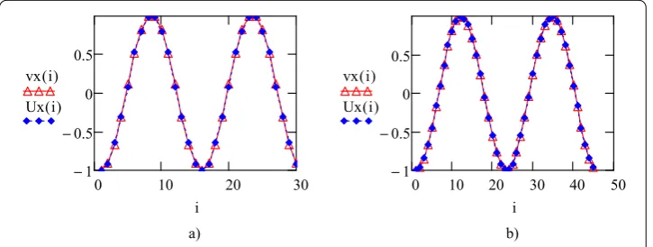
We can choose different values for the boundary elements numberNand for the trun-cation parametereps. For making the comparison, we consider first nodes, then nodes, for the boundary discretization, andeps= –.
In Figure the numerical values and the exact ones for the component of the velocity alongOxaxis are represented. In Figure a comparison between the numerical values of the component alongOyaxis and the exact ones is made. For the nodal values of the local pressure coefficient, the comparison is made in Figure .
As we can see from the three graphics, we get a good accuracy for the numerical solution.
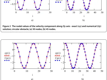
Figure 2 The nodal values of the velocity component alongOyaxis - exact (vy) and numerical (Uy) solution; circular obstacle; (a) 30 nodes; (b) 45 nodes.
Figure 3 The nodal values of the local pressure coefficient - exact (cp) and numerical (Cp) solution; circular obstacle; (a) 30 nodes; (b) 45 nodes.
Figure 4 The numerical values of the velocity components (Ux,Uy) and the local pressure coefficient (Cp); circular obstacle;M= 0.6; 45 nodes.
The computer code can deal with the case of compressible fluid flows, so numerical solutions for different values of Mach number can be obtained, cases when exact solutions are not known. In Figure the numerical solution for the case of a circular obstacle, when nodes are used for the boundary discretization andM= ., is performed.
boundary isz=x+iy,x=acost,y=bsint, at zero incidence angle,Fis given by
F(z) = U∞
z+√z–c+z–√z–c(a+b)
a–b
, wherec=a–b. ()
Thus, the dimensionless velocity components are given by the following relations:
u(z) = – +Rew(z), v(z) = –Imw(z), wherew(z) =
+√ z z–c +
–√ z z–c
a+b a–b
. ()
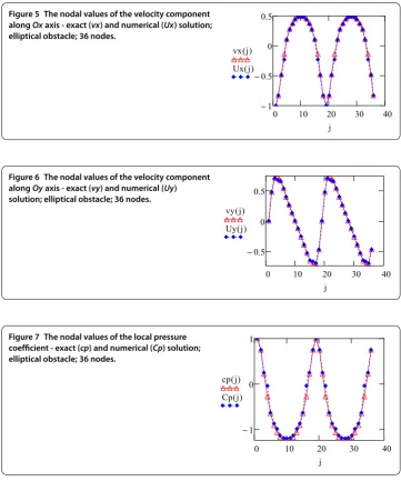
We consider in this paper an elliptical obstacle witha= andb= .
In Figures -, the comparisons between the numerical and the exact solutions for the case when we use nodes on the boundary (only boundary elements) are presented.
Figure 5 The nodal values of the velocity component alongOxaxis - exact (vx) and numerical (Ux) solution; elliptical obstacle; 36 nodes.
Figure 6 The nodal values of the velocity component alongOyaxis - exact (vy) and numerical (Uy) solution; elliptical obstacle; 36 nodes.
As in the case of a circular obstacle, we can see a great accuracy between the numerical solution and the exact one, even if using only cubic boundary elements for the boundary discretization.
The comparisons have shown that the numerical values of the nodal components of the velocity and of the local pressure coefficient and the exact ones are in good agreement even for a small number of nodes used for the boundary discretization. The analytical checking validates the exposed method and also the computer code.
The effectiveness of the boundary element method is clearly dependent on the imple-mentation of efficient and accurate integration procedures to evaluate boundary integrals of the singular kernels. The herein paper points out that the accuracy of the numerical solution is good in the case of using cubic boundary elements for the boundary discretiza-tion and the truncadiscretiza-tion method for singular integrals evaluadiscretiza-tion. Moreover, the truncadiscretiza-tion method is a method very easy to apply and to implement into a computer code.
Better results can be obtained when using more nodes for the boundary discretization, or a smaller value forepsparameter, but the computational effort is bigger when more nodes are used, and so, for obtaining a good ration accuracy/computational effort, we have to choose a certain range of values for the number of nodes.
Numerical integration is always a much more stable and precise process than numeri-cal differentiation and, if we formulate integral equivalent representations using primary functions when applying boundary element method, no differentiation of numerical quan-tities is needed, which is the fact that influences the accuracy of the numerical solution.
All this recommend the boundary element method, with boundary formulation which implies primary variables, as an efficient numerical technique to solve boundary value problems.
Competing interests
The author declares that she has no competing interests.
Acknowledgements
Dedicated to Professor Hari M Srivastava.
The author thanks the reviewers for their valuable suggestions and useful comments, and thus for their help in the improvement of the original manuscript.
Received: 14 December 2012 Accepted: 15 March 2013 Published: 8 April 2013
References
1. Banarjee, PK, Mukherjee, S (eds.): Developments in Boundary Element: Methods-3. Elsevier, Barking (1984) 2. Banarjee, PK, Watson, JO (eds.): Developments in Boundary Element: Methods-4. Elsevier, Barking (1986) 3. Bonnet, M: Boundary Integral Equation Methods for Solids and Fluids. Wiley, New York (1995)
4. Brebbia, CA, Telles, JCF, Wobel, LC: Boundary Element Theory and Application in Engineering. Springer, Berlin (1984) 5. Brebbia, CA, Walker, S: Boundary Element Techniques in Engineering. Butterworth, London (1980)
6. Ferziger, JH, Peric, M: Computational Methods for Fluid Dynamics, 2nd revised edn. Springer, Berlin (1999) 7. Carabineanu, A: A boundary element approach to the 2D potential flow problem around airfoils with cusped trailing
edge. Comput. Methods Appl. Mech. Eng.129, 213-219 (1996)
8. Drago¸s, L, Dinu, A: Application of the boundary element method to the thin airfoil theory. AIAA J.28, 1822 (1990) 9. Drago¸s, L, Dinu, A: A direct boundary integral method for the two-dimensional lifting flow. Arch. Mech.47, 813 (1995) 10. Katz, J, Plotkin, A: Low Speed Aerodynamics. Cambridge University Press, Cambridge (2001)
11. Drago¸s, L: Mathematical Methods in Aerodinamics, chap. 4, pp. 125-168. Romanian Academy Publishing, Bucure¸sti (2000)
12. Grecu, L: A solution of the boundary integral equation of the theory of infinite span airfoil in subsonic flow with linear boundary elements. Ann. Univ. Buchar., Math. Ser.LII(2), 181-188 (2003)
13. Grecu, L, Demian, G, Demian, M: Different kinds of boundary elements for solving the problem of the compressible fluid flow around bodies - a comparison study. In: Proc. of the World Congress on Engineering, London. Lecture Notes in Engineering and Computer Science, vol. II, pp. 972-977 (2008)
16. Vladimirescu, I, Grecu, L: Weakening the singularities when applying the BEM for 2D compressible fluid flow. In: Proc. of the International Multiconference of Engineers and Computer Scientists, Hong Kong. Lecture Notes in Engineering and Computer Science, pp. 2224-2229 (2010)
17. Drago¸s, L: Fluid Mechanics I, Part II: Ideal Incompressible Fluid, chap. 5, pp. 107-152. Romanian Academy Publishing, Bucure¸sti (1999)
doi:10.1186/1687-2770-2013-78