Enabling modeling framework with surrogate modeling capabilities and complex networks

(1)

Curriculum 1. Ci

vil and Environment

al Engineering

Francesco Sera

ﬁ

n

Enabling modeling framework with

surrogate modeling capabilities and

complex networks

Doctoral School in Civil, Environmental and

Mechanical Engineering

2019

- Doc

tor

al the

(2)

Except where otherwise noted, contents on this book are licensed under a Creative Common Attribution - Non Commercial - No Derivatives

4.0 International License

I

University of Trento

Doctoral School in Civil, Environmental and Mechanical Engineering http://web.unitn.it/en/dricam

Via Mesiano 77, I-38123 Trento

(3)

UNIVERSITY OF TRENTO

Department of Civil, Environmental and Mechanical

Engineering

Enabling modeling framework with

surrogate modeling capabilities and complex networks

Dissertation

submitted in partial satisfaction of the requirements for the degree of

Doctor of Philosophy

in Civil and Environmental Engineering

by

Francesco Serafin

Supervisor: PhD Prof Riccardo Rigon

Co-Advisor: PhD Olaf David

(4)

(5)

C O N T E N T S

1 introduction 1

1.1 Problem statement 1

1.1.1 Motivations 2

1.1.1.1 Issues related to the use of mathematical models

on the field 3

1.1.1.2 Issues related to the use of mathematical models

in research environments 5

1.2 Summary 9

2 background work and significance 11

2.1 Background work 11

2.1.1 Background work to facilitate operational use of

environ-mental models for service delivery organizations 11

environ-mental models in research environments 15

2.2 Context 19

2.3 Scope 20

2.4 Objectives statement 21

2.5 Relevance 22

2.6 Summary 23

3 surrogate modeling 25

3.1 Literature review 26

3.2 Research questions 28

3.3 Research design and Methods 29

3.3.1 Methodological approach 30

3.3.1.1 NeuroEvolution of Augmenting Topologies

(NEAT) 30

3.3.1.2 Feature selective NEAT 36

3.3.1.3 Ensemble of surrogate models and uncertainty

quantification 38

3.3.1.4 Framework-enabled NEAT based Surrogate

mod-eling (FeNS) 38

3.3.2 Technical approach and implementation 45

3.3.2.1 MongoDB 45

3.3.2.2 Microservice architecture and RESTful

API 47

3.3.2.3 Cloud Service Integration Platform (CSIP) 50

3.3.2.4 Encog 54

3.3.2.5 Surrogate Model Services implementation 55

3.4 Case studies 81

3.4.1 RUSLE2 82

3.4.1.1 DoE 1 82

3.4.1.2 DoE 2 86

3.4.1.3 DoE 3 92

3.4.1.4 Conclusions 98

3.4.2 Agricultural Ecosystem Services (AgES) 99

3.4.2.1 DoE 100

3.4.2.2 Conclusions 104

3.5 Summary 105

(6)

ii contents

4 complex network based physical modeling 107

4.1 Introduction 107

4.1.1 River network - graph structure analogy 109

4.2 Literature review 110

4.3 Research questions 111

4.4 Research design and Methods 115

4.4.1 Methodological approach 115

4.4.1.1 Directed Acyclic Graph data structure

(DAG) 115

4.4.1.2 Environmental Modeling Framework 119

4.4.1.3 Implicit parallelism 120

4.4.2 Technical approach and implementation 121

4.4.2.1 Object Modeling System v3 (OMS3) 121

4.4.2.2 Graph Modeling Structure: NET3 147

4.5 Case studies 167

4.5.1 GEOframe: Monitoring hydrological extremes 168

4.5.1.1 Application 168

4.5.1.2 NET3 additional features 168

4.5.2 GEOframe: JSWMM 171

4.5.3 FICUS: System of systems of models 174

4.6 Summary 176

5 conclusion 177

5.1 FeNS: conclusion and future development 177

5.2 NET3: conclusion and future development 179

a increasing complexity 181

a.1 SWAT 182

a.1.1 User experience 183

a.1.2 Software metrics 185

a.2 SWMM 187

a.2.1 User experience 188

a.2.2 Software metrics 189

b r and python annotation bindings for oms 193

b.1 Introduction 194

b.2 User experience 194

b.3 Technical approach and implementation 197

b.3.1 R back-end: Rserve 198

b.3.2 Python back-end: Jep 198

b.4 Docker image bundle 198

b.4.1 OMS R packages management 199

b.4.2 OMS Python packages management 199

b.5 Applications 199

b.5.1 RUG model 200

b.5.2 TRANSIMS model 200

b.6 Conclusions 201

(7)

L I S T O F F I G U R E S

Figure 1 OMS-compliant modeling solution that implements the

wa-ter budget as theory of embedded reservoir, creditBancheri

(2017). 8

Figure 2 Schematic to represents evolution of research models

from stand-alone applications to encapsulated

framework-compliant components. This processed unified/simplified

user-model interface and model-model intercommunication,

and enabled model runs on high performance computing

environments. The arrow on the left side illustrates the

reduction of model approach complexity by standardizing

input/output formats, and the reduction of model

mainte-nance and development cost. 12

Figure 3 Schematic to represent sub service and database

depen-dencies of CSIP-R2. The overall dependencies are about

290GB in size. 13

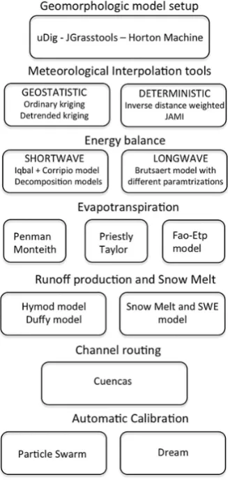
Figure 4 OMS-compliant components designed and developed by

Dr. Giuseppe Formetta and released in the initial version

of JGrass-NewAGE, creditFormetta et al.(2014a). 16

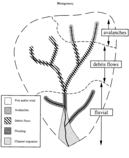
Figure 5 Schematic of watershed scale processes domains in a

mountain catchment, creditMontgomery(1999). 19

Figure 6 Schematic to represent current modeling practice. Research

scientists take advantage of the benefits of EMF

architec-tural design and modeling flexibility to release/deploy as

well as access conceptual/physical models; opposingly,

ser-vice delivery organizations make use of last enhancements

in terms of scientific knowledge and modeling practice

to provide stakeholders and policy makers with accurate

estimate of quantity of interest. 20

Figure 7 Schematic of actual contributions of this dissertation. A

new surrogate modeling layer is interpose to bridge the

gap between service delivery organizations and

conceptu-al/physical models. Contemporary, EMF modeling

capa-bilities are extended by implementing a graph modeling

structure. This allows for bridging the gap between

re-searcher scientists and modeling platforms by enabling

modelers creativity and elevating concept of modeling

en-capsulation and re-use. 22

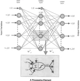
Figure 8 Single hidden layer feedforward neural network, credit

Govindaraju and Rao (2000a). 27

Figure 9 Competing conventions problem. The two ANNs have

identical structure but different order of hidden neurons.

Here, crossovering the two networks might result in missing

one of the 3 hidden units. 32

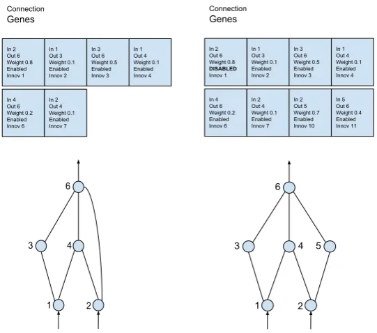
Figure 10 The genome (left side) maps the actual network structure

(right side). Two genes (node and connection) describe

neuron types and their interconnections. 33

(8)

iv list of figures

Figure 11 Example of add node mutation. Left hand side illustrates

the original ANN genotype and phenotype, while right

hand side illustrates ANN genotype and phenotype after

structural mutation. 34

Figure 12 Example of add link mutation. Left hand side illustrates

the original ANN genotype and phenotype, while right

hand side illustrates ANN genotype and phenotype after

structural mutation. 35

Figure 13 Process of two mating parents. 35

Figure 14 Left hand side shows the initial structure of NEAT

gener-ated ANN. Right hand side shows the initial structure of

a FS-NEAT generated ANN. 37

Figure 15 Dataset splitting in training, validation, and testing. 38

Figure 16 With respect to Figure 2, this schematic illustrates the introduction of a second step. In addition to framework

encapsulation, original research model runs generate SMs,

which can be used with little or no user effort and don’t

re-quire any model maintenance and development cost. 39

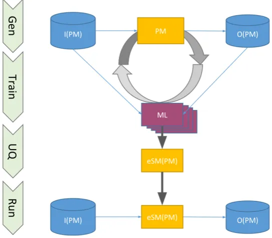
Figure 17 Generic FeNS concept. ML library employes original

model runs to emerge eSM from any modeling

solu-tion. 40

Figure 18 FeNS architectural design. FeNS-proxy interposes

be-tween user and model service, orchestrates parsing,

re-trieval and computing input/output original model

param-eters, and finally triggers surrogate model generation by

feeding FeNS-eSM with input/output snapshots. 44

Figure 19 CSIParchitecture, creditDavid et al. (2014a). 51

Figure 20 Set of 5 CSIP services that allows for generating the

SM. 56

Figure 21 Sequence diagram of CSIP-collect service. 57

Figure 22 Sequence diagram of CSIP-collect service when csv file is

attached. 60

Figure 23 Formal structure of MongoDB“raw” collection. 60

Figure 24 Sequence diagram of CSIP-normalize service. 61

Figure 25 Schematic of the Stages involved in the Feature Scaling

aggregator pipeline. 63

Figure 26 Sequence diagram of CSIP-normalize service when "raw"

and "valid" collection are available. 66

Figure 27 Formal structure of MongoDB "normalized"

collec-tion. 67

Figure 28 Conceptual approach of CSIP-train ensemble SMs. 68

Figure 29 Sequence diagram of CSIP-train service. 68

Figure 30 UML of implemented scaling mechanism. 70

Figure 31 Conceptual approach of CSIP-validation service. 73

Figure 32 Formal structure of MongoDB "trained.files"

collec-tion 74

collec-tion 75

collec-tion 76

Figure 35 Sequence diagram of CSIP-select service. 77

Figure 36 UML of implemented selection mechanism. 78

(9)

list of figures v

Figure 38 Sequence diagram of CSIP-run service. 79

Figure 39 Geographic distribution of the Corn Belt, credit (Green et al.(2018a)). 83

Figure 40 Cherokee county in Iowa. 84

Figure 41 Generic SM input/output structure for DoE 1. 84

Figure 42 Red crosses represents SM estimates, while black dots

represents original RUSLE2 runs. 85

Figure 43 Scatterplot of SM estimates against RUSLE2

re-sults. 86

Figure 44 Buena Vista and Clay counties in Iowa. 87

Figure 45 Generic SM input/output structure for DoE2. 88

Figure 46 Expert modules design for DoE2. 89

Figure 47 Cluster 1. Boxplots represents the ensemble of SMs

esti-mates against RUSLE2 erosion runs (red crosses). 90

Figure 48 Cluster 1. Scatterplot of SM estimates (computed on

the median of each boxplot) and RUSLE2 simulated

val-ues. 90

val-ues. 91

Figure 51 Buena Vista, Cherokee, Clay and Wrigth counties in

Iowa. 93

Figure 53 Expert modules design for DoE3. 95

val-ues. 96

val-ues. 97

val-ues. 98

Figure 60 SFIR watershed across Wright, Franklin, Hamilton, and

Hardin counties, creditGreen et al.(2018b). 99

Figure 62 Boxplots represents the ensemble of SMs estimates against

AgES runoff computations (red squares). 102

Figure 63 Scatterplot of SM estimates (computed on the median of

each boxplot) and AgES simulated values. 102

(10)

vi list of figures

each boxplot) and AgES simulated values. 104

Figure 68 Representation of the river network - graph structure

anal-ogy, credit Bancheri(2017) 109

Figure 69 Generic schematization of a hydropower plant. Part of the

stored water flows through the penstock from the dam, while

the remaining flow through the diversion reach. Credit,

Palen Lab blog. 113

Figure 70 Schematization of OMS3 architectural design, creditDavid et al.(2013). 123

Figure 71 Execution phases, and data flow of OMS3 modeling

solu-tion, credit David et al.(2013) 126

Figure 72 UML of OMS3 available modeling simulation types. 129

Figure 73 Usage example of @In annotation, credit David et al.

(2013). 138

Figure 74 Usage example of @Outto @Incomponent fields connec-tion, credit David et al.(2013). 140

Figure 75 NET3 conceptual design. From a single OMS3

mod-eling solution to interconnected and intercommunicating

modeling solutions. 147

Figure 76 NET3 conceptual design. Every node of the graph

model-ing structure runs a different modelmodel-ing solution to better

fit physical processes description. Intercommunication

be-tween modeling solutions happens with unlimited number

of variables. 147

Figure 77 UML of NET3 DiGraphclass. 148

Figure 78 NET3 family concept. 149

Figure 79 UML of search algorithm data structures. 154

Figure 80 Concept of search upstream or downstream. 155

Figure 81 UML of OMS3 available modeling simulation types. 156

Figure 82 Generic factory method design pattern, credit Gamma

(1995). 158

Figure 83 UML of NET3 factory method design pattern. 159

Figure 84 UML of OMS3 available modeling simulation types

in-cluding NET3. 162

Figure 85 Webgis front-end, creditBancheri et al. (2018a). 168

Figure 86 HRUs, creditBancheri et al. (2018a). 168

Figure 87 Multi-site calibration, creditBancheri et al.(2018a). 170

Figure 88 GEOframe validation at Ponte La Marmora, creditBancheri et al.(2018a) 171

Figure 89 GEOframe validation at Agri SS106, creditBancheri et al.

(2018a) 171

Figure 90 NET3-JSWMM component granularity, credit Dalla Torre et al.(2018);Dalla Torre (2019). 172

Figure 91 JSWMM modeling results, Dalla Torre et al. (2018);

Dalla Torre (2019) 173

Figure 92 FICUS SSoM conceptual design. 175

Figure 93 SSoM results displayed from the FICUS-UI. 175

Figure 94 NET3 Graph of Graphs conceptual design. 176

Figure 95 Trend of number of input files required for running a SWAT

(11)

list of figures vii

Figure 96 Trend of number of input parameters to setup for running

a SWAT simulation over official releases. 184

Figure 97 Trend of number of lines of source code (blue line) and

comments (red line) in SWAT code base over official

re-leases. 185

Figure 98 Trend of number of lines of files of the SWAT code base

over official releases. 186

Figure 99 Percentage of number of added, modified, removed, and

unchanged lines of code between SWAT consecutive

offi-cially released versions. Percentages are computed on the

older version. 187

Figure 100 Trend of number of lines of source code (blue line) and

comments (red line) in SWMM code base over officially

released versions. Left Y axis shows the magnitude of the

number of lines of code, right Y axis shows the magnitude

of the number of lines of comments. 189

Figure 101 Percentage of number of added, modified, and removed lines

of code between SWMM consecutive officially released

versions. 190

Figure 102 RUG modeling solution: Java components in light orange,

R OMS-compliant components in light blue. 200

Figure 103 TRANSIMS sample modeling solution: Java component in

light orange, Python OMS-compliant component in light

(12)

(13)

L I S T O F TA B L E S

Table 1 Modified table from Rizzoli et al. (2006) illustrates matches between model user types (rows) and their roles

(columns). 2

Table 2 Standard API exposed by a generic public class

Di-Graph. 117

Table 3 Standard API exposed by a generic public class

SearchAlgo. 118

Table 4 Comparison between heavyweight (traditional) and

lightweight frameworks, creditLloyd et al.(2011). 124

Table 5 List of OMS3 provided statistical moments. 133

Table 6 List of OMS3 provided model efficiencies. 134

Table 7 Number of file, lines of code, and comments of SWAT over

official releases. 186

Table 8 Percentage of identical, modified, removed, and added

num-ber of lines of code between SWAT versions (percentage

computed on the older version). 187

Table 9 Number of file and lines of code of SWMM code base over

official releases. 190

Table 10 Percentage of modified, removed, and added number of lines

of code between SWMM versions (percentage computed

on the older version). 191

Table 11 R and Python available data types. 197

(14)

(15)

L I S T O F A L G O R I T H M S

1 Pseudo-code of FS-NEAT population initialization in Encog. . . 71

(16)

(17)

L I S T I N G S

3.1 JSON Object of a generic model input parameter. . . 42

3.2 JSON Object for STANDARD input parameter. . . 42

3.3 JSON Object for COMPUTED input parameter. . . 42

3.4 JSON Object for ADDITIONAL input parameter. . . 43

3.5 JSON Object for DEPENDENCY DERIVED input parameter. . . 43

3.6 JSON Object for OUTPUT parameter. . . 43

3.7 Example of aputDependencies method. . . 43

3.8 REST call to EFH2, creditDavid et al.(2014a). . . 53

3.9 JSON response from a CSIP-eft run, credit David et al.(2014a). . . 53

3.10 CSIP-compliant EFH2 model, creditDavid et al.(2014a). . . 54

3.11 Template JSON payload of CSIP-collect. . . 57

3.12 Template JSON payload of CSIP-collect to generate a common dedicated“validation” collection. . . 59

3.13 Template JSON payload of CSIP-normalize service. . . 61

3.14 MongoDB Java client of Feature Scaling aggregator pipeline. . . 62

3.15 Stage 1 code snippet. . . 64

3.18 Conditional operator leveraged in Stage 3. . . 65

3.22 Template JSON payload of CSIP-train service. . . 69

3.23 Template JSON payload of CSIP-select service. . . 76

3.24 Template JSON payload of CSIP-run service. . . 79

3.25 Generic JSON response of CSIP-run service. . . 80

4.1 Example of a POJO class turned into OMS-compliant component by accommodating OMS3 annotations. . . .125

4.2 OMS3 modeling solution formal structure. . . .127

4.3 Example of OMS3 modeling solution, creditRigon et al.(2016) and Bancheri(2017). . . .128

4.4 Example of resource section in OMS3 modeling simulation with list of single resources. . . .130

4.5 Example of resource section in OMS3 modeling simulation with array of resources. . . .130

4.6 Example of available options in the OMS3 plot sub-element. . . . .130

4.7 OMS3 plot element. . . .131

4.11 Example of OMS3 summary element with single statistic. . . .132

4.12 Example of OMS3 summary element with multiple statistics on a specified period of time. . . .133

4.13 Example of OMS3 efficiency implementing multiple methods. . . . .134

4.14 Results of OMS3 efficiency. . . .135

4.15 Example of output strategy provided in a OMS3 modeling simulation.135 4.16 Example of OMS3 model element extracted from Listing4.3, credit Rigon et al.(2016) andBancheri(2017). . . .136

(18)

xiv listings

4.17 OMS3 component sub-element formal structure. . . .137

4.18 Example of OMS3 component sub-element. . . .137

4.19 OMS3 parameter subelement formal structure. . . .137

4.20 Example of OMS3 parameter subelement. . . .137

4.21 Example of OMS3 parameter file. . . .138

4.22 Usage example of parameter subelement in OMS3 modeling simulation.139 4.23 OMS3 connect subelement formal structure. . . .139

4.24 Example of OMS3 connect subelement derived from Listing4.3. . . .139

4.25 Example of OMS3 logging subelement with logging level per com-ponent. . . .140

4.26 Example of OMS3 logging subelement with one dedicated compo-nent logging in addition to generic logging level. . . .141

4.27 Example of OMS3 logging subelement with generic logging level. .141

4.28 Implementation of Logging class in OMS-compliant component. . . .141

4.29 OMS3 invoke method in modeling simulation. . . .142

4.30 OMS3 run method. . . .143

4.31 OMS3 initialize reflective call. . . .143

4.32 OMS3 input parameter read in and set up. . . .143

4.33 OMS3 execute reflective call. . . .143

4.34 OMS3 finalize reflective call. . . .143

4.35 OMS3 generic implementation ofcallAnnotatedmethod. . . . .144

4.36 OMS3whileconditional execution. . . .144

4.37 OMS3 implicit parallelization. . . .145

4.38 OMS3 implicit parallelization. . . .146

4.39 NET3 declaration of vertices and edges data structures. . . .148

4.40 NET3 instantiation of vertices and edges. . . .148

4.41 Example of Java synchronized wrapper class. . . .148

4.42 NET3 Family private class. . . .150

4.43 NET3 Family private class. . . .150

4.44 NET3 vertex initialization. . . .151

4.45 NET3 family initialization. . . .151

4.46 NET3 post ordering. . . .151

4.47 NET3DiGraphreversing. . . .152

4.48 Breadth first path data structure implementation. . . .154

4.49 Depth first path data structure implementation. . . .154

4.50 Depth first path data structure implementation. . . .156

4.51 Upstream searching algorithm implementation. . . .157

4.52 Downstrean searching algorithm implementation. . . .157

4.53 NET3 graph search algorithm implementation. . . .158

4.54 NET3 encapsulation of depth first and breadth first. . . .160

4.55 Net3 DSL sim file. . . .161

4.56 Formal structure of NET3 search direction DSL. . . .162

4.57 Usage example of NET3 search direction DSL. . . .162

4.58 NET3 run method. . . .163

4.59 NET3 observer initialization. . . .164

4.60 NET3 observer notification. . . .164

4.61 NET3 ready for simulation check. . . .165

4.62 Example of a POJO class turned into OMS/NET3-compliant com-ponent by accommodating OMS3 and NET3 annotations. . . .165

4.63 inFluxes/outFluxes DSL usage example. . . .166

4.64 inFluxes formal structure. . . .166

4.65 outFluxes formal structure. . . .166

(19)

listings xv

4.67 NET3 flags calibrate extension. . . .170

4.68 NET3-JSWMM access to common data structure, creditDalla Torre et al.(2018);Dalla Torre(2019). . . .174

B.1 R OMS-compliant version of theAttractorAnalysis.R . . . .195

(20)

(21)

A C R O N Y M S

AgES AgroEcoSystem

AgES-W AgroEcoSystem-Watershed ANN Artificial Neural Network

API Application Programming Interface BFS breadth-first search

BSON Binary jSON

CCA Common Component Architecture CCP Cloud Computing Platform CE Cellular Encoding

CI continuous integration

CSIP Cloud Service Integration Platform CSU Colorado State University

CPU Central Processing Unit CV Cross Validation DAG Directed Acyclic Graph DEM Digital Elevation Model DFS depth-first search DoE design of experiments DOI Digital Object Identifier DSL Domain Specific Language DSS Decision Support System

EMF Environmental Modeling Framework eSM ensemble of surrogate models ESMF Earth System Modeling Framework ESP ensemble streamflow prediction FD-NEAT Feature Deselective NEAT

FeNS Framework enabled NEAT-based Surrogate modeling

FICUS Framework for Integrating the Complexity of Uncertain Systems FIFO First-In-First-Out

FS-NEAT Feature Selective NEAT

(22)

xviii listings

GA Genetic Algorithm

GIS Geofraphic Information System

GoF goodness of fit GoG Graph of Graphs

GMS Graph Modeling Structure

GPL General Purpose Programming Language GPU Graphics Processing Unit

GUI Graphical User Interface HRU hydrological response unit HTTP HyperText Transfer Protocol JAMI Just Another Model Interpolator JDK Java Development Kit

JSON JavaScript Object Notation JVM Java Virtual Machine LIFO Last-In-First-Out LOC Lines of Code

LOOCV leave-one-out cross-validation MA Microservice Architecture MaaS Model as a Service ML Machine Learning

MLPs Multilayer Perceptrons MPI message passing interface MSE Mean Squared Error NE NeuroEvolution

NEAT NeuroEvolution of Augmenting Topology NS Nash-Sutcliffe

OMS Object Modeling System

PDGP Parallel Distributed Genetic Programming POJO Plain Old Java Object

PRMS Precipitation-Runoff Modeling System PSO Particle Swarm Optimization

RAM random-access memory

(23)

listings xix

RMSE Root Mean Squared Error ROA Resource-Oriented Architecture ROTO Routing Outputs to Outlet RRS Reproducible-Research System RTE Run Time Environment

RUG Regional Urban Growth

RUSLE2 Revised Universal Soil Loss Equation, Version 2 SaaS Software as a Service

SE Software Engineering sGA Structured Genetic Algorithm SFIR South Fork Iowa River SM Surrogate Model

SOA Service Oriented Architecture SoC separation of concerns SSoM System of Systems of Models SVD Singular Value Decomposition SWA Southfork Watershed Alliance SWAT Soil & Water Assessment Tool SWE Snow Water Equation

SWMM Storm Water Management Model

SWRBB Simulator of Water Resources in Rural Basin TDD Test-Driven Development

TIN triangulated irregular network

TRANSIMS TRansportation ANalysis SIMulation System TV training+validation

TWEANN Topology and Weight Evolving Artificial Neural Networks WPS Web Processing Services

UML Unified Modeling Language URI Uniform Resource Identifier

USDA United Stated Department of Agriculture

USDA-ARS United States Department of Agriculture - Agricultural Research

Service

USDA-NRCS United States Department of Agriculture - Natural Resources

Conservation Service

(24)

(25)

A B S T R A C T

Conceptual and physically based environmental simulation models as products

of research environments efforts became complex software over time in order to

allow describing the behaviour of natural phenomena more accurately. Results

from these models are considered accurate but often require to operate an entire

system of modeling resources with dedicated knowledge, an extensive set up, and

sometimes significant computational time. Model complexity limits wide model

adaptation among consultants because of lower available technical resources and

capabilities. However, models should be ubiquitous to use in both research and

consulting environments.

This dissertation aims to address and alleviate two aspects of research model

complexity: 1) for researchers, the model design complexity with respect to its

internal software structure and 2) for consultants, the model application complexity

with respect to data and parameter setup, runtime requirements, and proper model

infrastructure setup. The first contribution provides modeling design and

implemen-tation support by managing interacting modeling solutions as “Directed Acyclic

Graph”, while the second one helps to create surrogate models of complex physical

models as a streamlined process.

Both contributions are implemented within the Object Modeling System

(OMS)/Cloud Service Integration Platform (CSIP) modeling framework and in-frastructure and were applied in various studies.

First, a Machine Learning (ML)-based surrogate model approach is presented to respond to field application requirementes to get quick but "accurate enough"

model results with limited input and limited a-priori knowledge of the internal

physical processes involved. The surrogate model aims to capture the behaviour of

a physical model as an ensemble system of Artificial Neural Network (ANN). Here, the NeuroEvolution of Augmenting Topology (NEAT) technique has been leveraged because of its integration of a genetic approach to build and evolve itsANNs during supervised training. Throughout this phase, the thorough design of the services

facilitate seamless monitoring of structural mutations of the artificial neural network

and its performances with respect to behavioural emulation of the original model

response. This results in a streamlined surrogate model generation. Furthermore,

the stochasticity inherent to the evolutionary genetic algorithm combined with

a specially designed cross-validation approach allows for straightforward use of

the ensemble application. Several, slightly different artificial neural networks

are concurrently trained. The ensemble system is built upon the selection of the

utmost performant surrogate models and is used collectively to provide uncertainty

quantified results when applied against new data.

Secondly, a Directed Acyclic Graph (DAG) modeling structure NET3 was de-veloped. NET3 provides appropriate data structures to represent modeling states

interactions as relationships based on network topologies. The inherent structure

of theDAGcommands the execution of modeling tasks. NET3 implicitly manages the parallel computation depending on the network topology. A node of a NET3

modeling structure encapsulates any sort of modeling solution such as a system

of ordinary differential equations, a set of statistical rules, or a system of partial

differential equations. Each link connects these modeling solutions by handling their

(26)

xxii listings

data flow. As a result, NET3 simplifies 1) the translation of physical mathematical

concepts into model components, and 2) the management of complex interactions

of modeling solutions. NET3 also pushes forward the idea of separating concerns

between software architecture and scientific model codebase. It manages aspects

that relate to the architectural design of the graph modeling structure and lets

research scientist focus on their model’s domain. NET3 improves encapsulation

and reusability of scientific/mathematical concepts. It avoids code duplication by

allowing the same modeling solution to be adopted in different nodes and finely

adapted to specific requirements. In summary, NET3 enables a new level of

model-ing flexibility by allowmodel-ing to quickly change model representations to explore new

modeling solutions.

The two presented contributions were integrated into the OMS/CSIP

Environmental Modeling Framework (EMF)/Cloud Computing Platform (CCP).

EMFs are standard practice in environmental modeling because they represent a software solution of separating the burden of software architectural design

manage-ment from scientific research.

Here,OMS/CSIPhas been identified“advanced” in terms ofEMFs design. It offers high flexibility, low language invasiveness, fine and thorough architectural

design, and innovative cloud computing deployment infrastructure. These aspects

makeOMS/CSIPinfrastructure the suitable platform to hostNEATbased surrogate modeling and NET3 extensions. Framework enabled NEAT-based Surrogate

modeling (FeNS) results from the full integration ofNEATbased surrogate modeling approach with OMS/CSIP platform. Here, the surrogate model approach was developed asCSIP services to help transitioning from research models to “field models” _{by enabling the modeling framework to interact with}_CSIP_services, _ML libraries, and a NoSQL database to emerge model surrogates for a(ny) modelling

solution. OMSCSIP was extended to harvest data from each model run and automatically derive the surrogate model at the modeling framework level. NET3

extendsOMSmodeling simulations to run as a graph network of interconnected modeling solutions. Furthermore, it enhances availableOMScalibration algorithms to become multi-site calibration procedures.OMSalready provided implicit parallel computation of independent components in a modeling solution. NET3 now adds a

further layer of implicit parallelism by concurrently running independent modeling

solutions.

Two studies were carried out to develop and testFeNSwhile three applications supported the development and testing of NET3.

Surrogate models of the Revised Universal Soil Loss Equation, Version 2

(RUSLE2) were generated to scale up from simple test cases with a constrained input space to more generic applications including a larger variety of input

parame-ters. The main goal of the surrogate model was to streamline and simplify access

to theRUSLE2model behaviour. We performed sensitivity analysis ofRUSLE2

to limit the input space to only relevant parameters (e.g. soil properties, climate

parameter, field geometries, crop rotation description). The main study area was

the State of Iowa starting from a single county (Clay county) ending up to four

counties (Buena Vista, Cherokee, Clay, and Wright). Clustering methodologies

were applied to improve surrogate model accuracy and to accelerate the training

process by reducing the dataset size. The overall “goodness-of-fit” against the

testing dataset estimated on the median of the uncertainty quantified result of the

surrogate models ensemble was always above 0.95 Nash-Sutcliffe (NS), Root Mean Squared Error (RMSE) between 0.13 and 0.36, and bias between -0.07 and 0.02. In many cases, accuracy of the surrogate model with respect to testing dataset was

(27)

listings xxiii

Surrogate models of the AgroEcoSystem (AgES) were generated to apply and test FeNSmethodology to a semi-distributed hydrologic model. The main goal of the surrogate model was to streamline and simplify access to the AgES model

behaviour. Only relevant lumped parameters on watershed centroid were used to

train the surrogate models and limit the input space to only relevant parameters (e.g.

precipitation, groundwater level, LAI, and potential evapotranspiration). The main

study area was the South Fork Iowa River (SFIR) watershed in the State of Iowa across Wright, Franklin, Hamilton, and Hardin counties. The overall“goodness-of-fit”

against the testing dataset estimated on the median of the uncertainty quantified

result of the surrogate models ensemble was above 0.97 NS,RMSEof 2.24, and bias of -0.0794.

With respect to NET3, the first application is the real-time modeling of flood

forecasting through GEOframe system for the Civil Protection of Regione Basilicata

implemented by PhD Bancheri. To scale the computation and finely tune calibration

parameters, the Basilicata river basins were split into subcatchments where each

was represented by a different NET3 node.

The second application was part of Mr. Dalla Torre’s master ’s thesis where the

computational core of the rainfall-runoff model of Storm Water Management Model

(SWMM by EPA) was componentized. NET3 now allows for reimplementing a

concise and lightweight SWMM modeling core and highly parallel model runs.

Software architectural design of rainfall-runoff, routing and sewer pipe design

components targeted separation of concerns, single responsibility, and encapsulation

principles. It resulted in clean and minimized code base. NET3 manages component

connections and scalable computation by hosting rainfall-runoff modeling solution

into separated nodes from routing and sewer pipe design modeling solution. It also

enables each node of the modeling structure to 1) access a shared data structure to

fetch input data from and push results to (SWMMobject), and 2) internally analyze

the upstream subtree in order to adjust sewer pipe design parameters.

The third test case is the application of a System of Systems of Models (SSoM) where each node of the graph modeling structure encapsulates a single responsibility

system of urban models. Because of the stochasticity involved in each system of

models, the entire graph modeling solution was required to run several times and

generate independent realizations. Hence, NET3 was enabled to run a Graph of

(28)

(29)

1

I N T R O D U C T I O N

(Beasley et al.(1980)), CASC2D (Julien and Saghafian(1991)), GLEAMS (Leonard et al.(1987)), SWAT (Arnold and Allen(1999)), RZWQM (Team et al.(1998)), WEPP (Laflen et al. (1991)), MODFLOW (Harbaugh et al.(2000)), WAMS (DePinto and Rodgers(1994)) integrated GIS (GRASS (Goran et al.(1983);Ehlschlaeger(1989);

Westervelt et al.(1991)) in these specific cases) interfaces and algorithms in their modeling core (Cronshey et al.(1993);Rewerts and Engel(1991);Krummel et al.

(1996);Hay et al.(1993);Srinivasan(1992);Srinivasan et al.(1998);Arnold et al.

(1995)). Since then, mathematical models and GIS capabilities developed along together. Practical examples are the management and integration of satellite

imagery and data assimilation techniques in the standard usage of process-based

models (Akinmolayan et al.(2018);Anees et al.(2018);Bayramov et al.(2019)).

In the next section, a deeper analysis of the identified problem is performed.

Solid bases and motivations are provided to support the relevance of this research.

1.1.1 Motivations

Conceptual/physical models should be ubiquitous to use in both research and

consulting environments. Rizzoli et al.(2006) correctly summarizes model user types and roles (Table1is a slightly modified version ofRizzoli et al.(2006)). However, no model actually fits requirement from every user and role simultaneously.

Users

Roles Hard

Coders Soft

Coders

Linkers

Run-ners

Player

View-ers Providers

Prime 4 4

Other End Users 4 4 4 4

Technical 4 4 4

Researchers 4 4 4 4 4

Table 1:Modified table fromRizzoli et al.(2006) illustrates matches between model user

types (rows) and their roles (columns).

The use of numerical models in both scientific and consultant environments is

challenging because of a number of issues. The analysis of these issues motivated

this research. However, before going into details of each issue, it is important to

understand the meaning of“operational use”in research and consultant communities.

Service delivery organizations and consultant companies are mainly end-users

of mathematical models. Their goal is to leverage software features to provide

stakeholders and decision makers with accurate information in topic like conservation

practices (e.g. land management and crop operations to avoid excessive soil erosion),

prediction of quantity of interest (e.g. water quantity for electric power plan

manoeuvres), etc.

They don’t develop or maintain software, they are not capable or interested in

improving numerical methods, conceptual design or physical process representations

due to lack of expertise and resources. Furthermore, from an IT perspective,

they may not have in-house computing environments available to run and deploy

modeling software. Consequently, they have to rely on third-party environments

and personnel.

In research environments,“operational use” means both maintenance/development

and application of mathematical models.

Model development involves the integration of last enhancements in conceptual

(31)

1.1 problem statement 3

of integrated tools like GIS capabilities are an important part of model evolution.

IT development involves integration and maintenance of modeling frameworks, db

connections and design, and proper development to keep up with last innovations, e.g.,

cloud computing, scalability on computer clusters and super-computing environments

in general.

The application side involves model testing and state-of-art consultancy exercises

to solve particular problems. In this case, high expertise is available to deal

with complex scientific debugging procedures and results interpretation, input data

management and preparation, calibration and sensitivity analysis procedures (Green et al. (2015)). Complete model understanding allows for identifying conceptual, mathematical/numerical problems and modeling inaccuracies and finely tuning input

parameters and mathematical aspects, thoroughly testing each and every model

capability.

Unfortunately, smaller research groups cannot rely on suitable IT expertise

in order to properly design, develop, and maintain big complex models. Past

experiences show how lacking of proper software architecture design ends up with

chaotic, hardly developable and readable/debuggable code bases (Rizzoli et al.

(2006);David et al. (2013);Formetta et al.(2014a)). Which in turn slows down research advancements.

Now that the concept of“operational use” in both environments has been

intro-duced and described, it’s easier to understand that there are issues related to daily

use of conceptual and physical models. And these issues are, nevertheless, different.

Consequently, this problem statement deepens issues analysis in two different

subsections. The next subsection identifies and describes issues related to the

operational use of mathematical models on the field or in consultant agencies.

Subsequently, issues related to operational use of mathematical models in research

environments are tackled.

1.1.1.1 Issues related to the use of mathematical models on the field

Environmental models are regularly applied by consultant agencies and

on-the-field personnel. However, daily use is not effortless due to a series of constraints

and issues that are following analyzed.

Rainfall-runoff modelling may serve as an example here. Rainfall-runoff is a

highly nonlinear, spatially heterogeneous, and very complex process (Srinivasulu and Jain(2009);Beven(2011)) which is comprised of several different, interconnected processes, some of which are not clearly understood yet (Hrachowitz and Clark

(2017);Young and Leedal(2013);Zhang and Govindaraju(2000);Porporato and Ridolfi (2001)). The modeling approach evolved over time from a pure empirical form (the Rational Method is the first empirical model ever published in 1851,

developed by Thomas Mulvaney), through conceptual models (first models dates

back to 1960s, when simplified equations describing hydrological processes were

numerically integrated thanks to increased computational power (Wheater et al.

(2012);Beven(2011)), to a fully physically based one (1970s computational power was such to solve partial differential equations (Wheater et al.(2012);Beven(2011);

Wagener et al.(2004)). Strengths of empirical models are small input parameter sets required and a fast model runtime. However, they lack result accuracy and physical

understanding of involved phenomena. The need of comprehensive understanding of

physical processes at different scales pushed research efforts toward the development

of conceptual models first and fully physically based consequently.

Conceptual models are built upon a conceptual representation of the analyzed

(32)

4 introduction

ordinary differential equations, and, in the case of rainfall-runoff models, schematized

through interconnected reservoirs (Bancheri et al.(2019)). This allows on-the-field personnel to easily understand the model behaviour. However, the implemented

equations involve a number of parameters that are not directly or physically

measurable. Thus, complex calibration procedures are necessary to estimate those

parameters for a specific catchment. Here, the“equifinality” problem arises (Beven

(1993)): different combinations of parameter values may fit observed data especially when available data have restricted information content and the performance criterion

is based off of a single objective function (Wheater et al.(2012)). Then it is impossible to uniquely identify the model structure and apply it to ungauged catchments. When

calibration procedures cannot solve the non-identifiability problem (Beven (1993)), a single set of parameters cannot be estimated. In this case, Generalized Sensitivity

Analysis (Spear and Hornberger (1980)) allows to select “behavioural” set of parameters according to observed data (Wheater et al.(2012)). Afterwords, the model output is uncertainty quantified and contribution of each input parameter

uncertainty evaluated (Wikipedia(2018)).

The equifinality problem has a smaller impact on simulation runs when it comes

to multi-criteria optimization. Here, additional information are available and

integrated into calibration procedures (Yapo et al.(1998);Wagener et al.(2001,

2000)). Nonetheless, modeling tool-kits support sensitivity analysis in order to investigate and identify the most suitable model structure and parameter uncertainty

(Wheater et al. (2012)).

In summary, conceptual models are easily understandable without specific

ex-pertise because of their abstract representation of the real world. However, they

require both calibration and sensitivity analysis procedures which involve several

model runs, setup of design of experiments, and final interpretation of parameter

estimate and model outputs.

Physically based or mechanistic models are built upon partial differential

equa-tions. The latter are the most accurate mathematical description of physical processes

(Wheater et al. (2012);Fatichi et al.(2016)). These equations are discretized as finite difference, finite elements or finite volumes over a spatial mesh and solved

numerically (Wheater et al. (2012);Pechlivanidis et al. (2011)). And research in this field is highly active (e.g. Casulli(2017), Tubini et al. (2017), andDumbser et al.(2019)) (Fatichi et al.(2016);Paniconi and Putti(2015)).

Physical models differ from conceptual models because input parameters are

actually state variables (Devia et al. (2015); Fatichi et al. (2016)). These have physical meaning and are actually measurable (Wheater et al.(2012)).

Theoretically these models should be used in ungauged catchments, with input

parameters estimated apriori. However, this practice is not directly achievable for

two reasons: (a) small-scale catchments and laboratory experiments are main sources

of the physics underneath these modes and make them not straightly applicables to

big catchments; (b) some parameters cannot be evaluated on the entire study area,

e.g. spatial heterogeneity of soil stratification. Thus, a comprehensive representation

of the study area in terms of input dataset is hardly feasible (Wheater et al.(2012);

Pechlivanidis et al.(2011)).

Here, calibration procedures can be useful when some input parameters are

unknown, even if they are not mandatory in a mechanistic model workflow.

Con-sequently, sensitivity analysis become useful as well in order to estimate model

uncertainty.

Nonetheless, these type of models need a big amount of detailed input information

to satisfy initial state requirements. They are really complex and high expertise is

(33)

dedicated supercomputing environments can speed up the computation only if model

architectural design account for parallel, or scalable algorithms (Devia et al.(2015)).

The analysis of the different available model types helps to summarize issues

and limitations on-the-field personnel and consultant agencies have to deal with in

order to apply conceptual and mechanistic models:

1. Thorough understanding of concerned model: both type of models require

in-depth understanding and expertise. Calibration and sensitivity analysis

procedures are fundamental parts in the entire setup of conceptual models.

Physics of the involved processes has to be perfectly clear when it comes

to setup physical model parameters. Otherwise, wrong usage of tools and

parameters setup can lead to incorrect and deceptive results. Planning

environments cannot always rely on these expertise.

2. Data collection and preparation: big dataset feed both type of models.

In conceptual models, they are mostly required for calibration procedures.

For mechanistic models instead, spatially distributed initial conditions and

study area characterizations are mandatory information. Technology evolution

allows to meet these needs by providing satellite data, finer grid raster

maps, low-error measuring instruments. However, these information are not

available everywhere and, if they are, data preparation and assimilation are

not trivial tasks and required dedicated proficiencies and GIS capabilities.

Additionally, the lack of input standards which especially concerns old models,

calls for the design of model-specific applications to convert raw data into

model-compliant inputs. As a result, data collection and preparation end up

being a long and tedious operation consultant agencies don’t always have

time and expertise required to deal with.

3. Run-time: both type of model simulations are computationally expensive.

Calibration and sensitivity analysis procedures require several conceptual

model runs to select the set of parameters that better fits observed data

or to estimate model uncertainty. Differently, physically based models are

computationally demanding because numerical methods return accurate results

on finer grids. Service delivery organizations usually need quick results even

if not the most accurate.

Furthermore, even if models are designed to take advantage of multi-processors

machines or computer clusters, service delivery organizations don’t usually

have physical access to supercomputing environments and cannot rely on

in-house proficiency to manage them. Yet, if supercomputing environments are

not available, relying on third-party machines and personnel with dedicated

expertise is expensive.

In summary, the analysis of issues related to daily use of conceptual or physically

based models in planning/consultant environments identifies three main topics: (1)

lacking of model understanding and expertise in order to fully manage and leverage

model capabilities; (2) the absence of required input dataset for feeding calibration

and sensitivity analysis procedures or time to handle and properly convert raw data

into model-compliant data; (3) unavailability of proper IT infrastructures to reduce

computational runtime or lacking of expertise to apply them.

1.1.1.2 Issues related to the use of mathematical models in research envi-ronments

Mathematical models result from research environment efforts. Here, “operational

(34)

6 introduction

1. model maintenance and development, which differs from software maintenance

and development since mostly target bug fixing of modelled processes and

integration of recent numerical and mathematical enhancements, rather than

software architecture refactoring;

2. model testing and application to advanced problems that have often never

been addressed before.

In both cases, scientists’ approach to research models is not straightforward and

the reasons are following described. A paragraph with a dedicated analysis for

each previously listed issue is provided. Paragraph1.1.1.2.1introduces to EMFs methodology as well, which is used throughout paragraph1.1.1.2.2.

1.1.1.2.1 Issue experienced during model maintenance and development

Research outputs are always up to state-of-art in terms of scientific content.

However, mathematical models historically lack of proper software engineering and

have been designed as monolithic code base. The latter has been identified as the

main cause of current difficulties in model development and maintenance (Formetta et al.(2014a);Rizzoli et al.(2006);David et al.(2013)). The introduction ofEMFs in modeling workflow alleviates source code maintenance and development. Yet,

EMFs actually limits modeler creativity.

Monolithic applications constraint collective model development, model sharing

and reusability because the code structure lacks of separation of concerns (Martin

(2009);Newman(2015)), which means that there are no boundaries between different scientific/mathematical concepts (David et al.(2013);Nadareishvili et al.(2016)). Consequently, a scientists needs deep understanding of the entire model to make

modifications and speed up the debugging process (Newman(2015);Nadareishvili et al.(2016)). In terms of deployment into production environment, just a single bug fix or modification of a single line of code of a monolithic application requires the

deployment of the entire software (Nadareishvili et al.(2016)). Not to mention the scalability issue: enabling a simple multithreading computation in a monolithic

software is complicated already, scalability on computer clusters even more (Newman

(2015);Nadareishvili et al.(2016)). As a result, leveraging state-of-art computer hardware solutions becomes a cumbersome and most likely unachievable goal.

There are several reasons why software architecture has always had low priority in

environmental model research. Historical, cultural, resource and reward constraints

have been identified byDavid et al.(2013) and are following summarized. From anhistoricalpoint of view, when the era of model development started, C and

FORTRAN were the most notable general purpose programming languages to begin

with. These languages rely on free and open source compilers and tools as well as

active developer communities. They are procedural programming languages though,

which already addresses software development towards monolithic architecture.

From a cultural standpoint, environmental modelers usually have self-taught

programming knowledge and low expertise in software design and architectural

patterns (David et al.(2013);Rizzoli et al.(2006)). Their biggest desire is to dive into deeper and more accurate descriptions of environmental processes, model them,

and implement them to test the improved modeling solution (David et al.(2013)). It is obviously not possible and fair to ask a natural resource scientist or engineer to

take care of both modeling development and software architecture design.

Here the third constraint comes up. A computer scientist, software engineer or

hydroinformatic engineer should take care of properly choosing the most suitable

software design by anticipating target architectures to support multi language

(35)

the refactoring of poorly designed modules (David et al.(2013);Rizzoli et al.(2006)). However,research budgets are typically limited and expertise of previous listed

professional figures are not usually accounted for.

The last constraint,rewards perspective, usually hinges to pure achievement of

result accuracy. Model reusability and long-term maintainability frequently have

low value and priority consequently.

Eventually, the highest quality scientific model codebase ends up being an

handcrafted monolith of thousands of lines of code, which is hard to refactor and

redesign (David et al.(2013)).

Several EMFs have been developed in the last decade in order to move the burden of software architectural design apart from pure scientific research. Some

of the most notable are: OpenMI (Blind and Gregersen(2005);Gregersen et al.

(2007)), Common Component Architecture (CCA) (Bernholdt et al.(2003)), Earth System Modeling Framework (ESMF) (Collins et al.(2005)), Common Modeling Protocol (Moore et al. (2007)), andOMS(David et al.(2013)).

EMFs are built upon the notion of component-based software development. They elevate the principle of separation of concerns by splitting responsibilities between

framework and components. A component is a typical object-oriented programming

concept where a class or module is the core building block of the entire application

(Peckham et al. (2013);David et al. (2013)). The framework enables a software “plug-ins” system where a series of precompiled components can be plugged in

or unplugged on necessity . It takes care of runtime component connections via

dynamic linking and other complicated tasks such as multi language interoperability,

multi-threading parallelization of algorithms, temporal-spatial stepping, etc. (David et al.(2013)).

Accordingly, a monolithic codebase can be refactored into a framework-compliant

set of components by extracting the scientific knowledge only and splitting it into

single responsibility functional units. Good software design practice identifies the

optimum level of component granularity into the encapsulation of a single physical

process per module, e.g. evapotranspiration, infiltration, runoff, etc. (Peckham et al.

(2013)). Working with higher or lower level of granularity is possible though and might be necessary in specific cases (Qu and Duffy (2007)). However, the “one conceptual/physical process per unit” design identify the most flexible granularity

level where scientists can easily swap out an old modeling methodology for an

innovative or a more appropriate one. Additionally, interfaces between components

and related framework connections become “physical domain boundaries” and “physical fluxes exchange” respectively, further elevating the concept of modeling

natural phenomena.

The benefits of employing an EMFin modeling workflow are streamlined model development, improved developer ’s software quality and reliability, time and cost

effectiveness, high level of modeling flexibility.

Several models are framework compliant already, e.g. GEOframe-NewAGE

(Bancheri(2017);Formetta et al.(2011);Formetta(2013);Formetta et al.(2013b,a,

2014a,b, 2016a,c); Abera et al. (2017a,b)), Precipitation-Runoff Modeling Sys-tem (PRMS) (Leavesley et al.(2005)),AgESand it predecessor AgroEcoSystem-Watershed (AgES-W) (Ascough II et al. (2012);Ascough et al.(2014);Green et al.

(2014,2015)), BioMA (Donatelli et al.(2012)), and TopoFlow (Peckham et al.(2017)). A deeper analysis of GEOframe-NewAGE to establish the upsides of modelling

with components is proposed in subsection 2.1.2 Background work to facilitate

operational use of environmental models in research environments_.

(36)

8 introduction

Figure 1:OMS-compliant modeling solution that implements the water budget as theory of embedded reservoir,

creditBancheri(2017).

This lets modeler exploring new problem solving approaches further widening the

boundaries of actual modeling techniques.

Figure1 is used here for the sake of example. It represents the OMS-compliant modeling solution designed byBancheri(2017) for testing the theory of embedded reservoir model developed during her doctoral research. It estimates the water

budget for a generic watershed.

This modeling solution is pretty flexible already: it allows for easily swapping

out a single conceptual/physical process, e.g. surface flow, with a different or maybe

simpler implementation. However, this modeling approach constraints a scientist to

model an entire watershed as an homogeneous entity.

If this is the case of a small watershed, a single modeling solution might match

scientist requirements already. It doesn’t properly work for a big watershed involving

mountain, hill, and plain subcatchments. Here, a modeler might want to finely

tune modeling solution parameters for each type of subcatchment. She/he might

also want to switch a specific module for a different component per each type of

subcatchment, or she/he might want to run completely different modeling solutions

in each subcatchment. Additionally, human artifacts such as power plant could

potentially become part of a complex modeling solution. But they require dedicated

mathematical model and possibly different time loops.

As a result, implementation of complex modeling solutions by leveraging actual

frameworks capabilities is not achievable. ActualEMFs functionalities limit mod-eler creativity and talent. CurrentEMFs capabilities push back the modeling of complex interconnections and related potential scalable computation to modeler

responsibilities.

1.1.1.2.2 Issue experienced during model testing and application to ad-vanced problems

The second issue encountered during regular operational use of

mathemati-cal models in research environments relates to actual application to state-of-art

consultancy problems.

In this particular case, scientists don’t usually have time constraints or lacking of

data compared to service delivery organizations. Consequently, application of full

mathematical model is achievable and actually fundamental: deep understanding of

physical processes allows for studying state-of-art problems and improving modeling

techniques eventually.

The constraints are rather on the steep learning curve a scientist has to deal

with while approaching a new model. Poor software design and lacking of software

(37)

1.2 summary 9

Research environments are still resistant to adoption of version control systems to

track software development, and code peer review is not usually part of standard

workflow (David et al. (2013)).

Additionally, a modeler might need to investigate the involved phenomenon

from different scales and perspectives, and experiment with modeling solutions

consequently. This research methodology requires modeling software to provide

high level flexibility to easily accommodate modeler creativity.

1.1.1.2.3 Summary of issues related to the use of mathematical models in research environments

Summarizing, the analysis of issues related to the daily use of conceptual

or physically based models in research environments identifies the necessity of

adopting EMFs in everyday workflow and the needs of improving their flexibility to:

1. facilitate model maintenance and development;

2. avoid error-prone code duplication;

3. improve modeler productivity and accommodate modeler creativity.

1.2 summary

The problem statement of this dissertation identifies issues related to the use

of mathematical models for (A) service delivery organizations and (B) research

environments.

Operational use of conceptual/physical models in service delivery organizations

means leveraging research modeling advancements as knowledge encapsulated

black-box to support stakeholders and decision makers’ questions with accurate

predictions and information.

However, consultancy agencies struggle to properly exercise research simulation

models since they may lack of (1) expertise to understand conceptual or physical

processes requirements to set up calibration or sensitivity analysis procedures;

(2) time to collect and prepare datasets to satisfy models high resolution input

parameter requirements; (3) in-house availability of computing environments to

deploy and exercise modeling simulations.

Operational use of conceptual/physical models in research environments means

codebase maintenance, implementation of modeling advancements, and design

of modeling simulations for state-of-art consultancy applications. In research

environments, a simulation model is a white-box since research scientists have

to implement last enhancements in conceptual design, or numerical/mathematical

and physical fields. Additionally, scientists need to dig into model implementation

when it comes to thoroughly tune calibration procedures and input parameters for

advanced applications.

However research scientists struggle to maintain and develop simulation model

code base since their are not software engineers, usually have self-taught

program-ming knowledge, and model design commonly lacks of accurate software architecture.

Furthermore, current modeling tools constraint modeler creativity and impede the

design of innovative modeling solutions.

Issues in both consultant agencies and research environments are getting more

(38)

10 introduction

growing due to integration of research enhancements, engineering practices and

additional capabilities such as GIS algorithms. A brief analysis of notable modeling

software (Soil & Water Assessment Tool (SWAT) and Storm Water Management Model (SWMM)), which have been developed for more than a decade, is available in Appendix A NET3: conclusion and future development to demonstrate this increasing complexity: SWAToverall increment of number of lines of code in about 15 years is more than 100%, whileSWMM source grew up of 40% in about 14 years.

The next chapter presents background work and material that attempted to

overcome identified constraints. The detailed analysis of current applications of

EMFs/CCPs in modeling workflows allows for identifying context and scope of this dissertation, introducing to research contributions proposed to solve identified

(39)

2

B A C K G R O U N D W O R K A N D

S I G N I F I C A N C E

research environments. Section 2.2 identifies the modeling core to intervene to, while Section2.3points to identified methodologies to expand modeling capabilities and flexibility. Section2.4introduces to the actual contributions of this dissertation and describes identified strategies to (1) facilitate access to model behaviour for

service delivery organizations, and (2) simplify model development and maintenance

and elevate modeler creativity for researchers and modelers. Finally, Section2.5

summarizes who will benefit from this research.

2.1 background work

The identified problems in service delivery organizations and research

environ-ments are well established and literature reveals that research work has been

done already while attempting to overcome limitations and constraints (David et al.

(2013);Peckham et al.(2013)).

This section focuses on analyzing background work that has been conducted so far.

Following the structure of this dissertation, background work related to operational

use of mathematical models in consultancy agencies is separately described from

background work related to operational use of mathematical models in research