8. Scheduling in a Single-Stage, Multi-Item Compatible Process Using Multiple ARC Network with Gains Model Using Excel Solver

(1)

Scheduling in a Single-Stage, Multi-Item Compatible Process

Using Multiple ARC Network with Gains Model Using Excel

Solver

Dr. Bokkasam Sasidhar*

Professor, College of Business Administration King Saud University, Riyadh, Kingdom of Saudi Arabia

* Corresponding author

1. Introduction

Microsoft Excel is bundled with every copy of Microsoft Excel and this widespread availability has spawned many applications in industry and government. Many spreadsheet models are created by functional managers who base them on the examples supplied with Excel or found in various books. In other cases, these spreadsheet optimization models are created by outside consultants with industry expertise, rather than OR/MS expertise per se. Users of Solver products are typically solving LP models in the range of several hundred to a few thousand (some as large as 10,000) decision variables and constraints (Daniel et al., 1998). It is estimated that 90 to 95 percent of these users have no affiliation with the OR/MS community. They are clearly "dispersed practitioners" (Geoffrion, 1991). Hence, optimization models may yield high economic value. (Thomas, 2009) has demonstrated how the use of Solver package in Microsoft Excel can be easily used to solve optimization problems in management accounting. (Eugénio and Romualdo, 2001) have shown how the Solver feature of the Excel spreadsheet can be used for the optimization of a fairly complex system, i.e., a classic solvent extraction/pollution prevention with heat integration process. The specific goal was the design optimization for continuous recovery of organic solvents using a gas absorption tower with solvent recovery in a stripper.

Decision networks, which involve a sequence of decisions, is gaining popularity among the management scientists (Saksena, 1982; 1985). Scheduling is a key factor for manufacturing productivity. Efficient scheduling can improve on-time delivery, reduce inventory, cut lead times and improve the utilization of bottleneck resources. Because of the combinatorial nature of the scheduling problems, it is necessary to use proper optimization tasks. In the literature there are various studies that focus on the efficient scheduling implementing approaches (Akturk and Ozkan, 2001; Morton and Pentico, 1993; Xue et al., 2001; Sun and Xue, 2001). In the past decade, a large number of optimization models and approaches have been proposed for batch scheduling and planning. A number of reviews on the planning and scheduling of batch processes have been presented in the literature (Pinto and Grossmann, 1998; Kallrath, 2002; Floudas and Lin, 2004; Burkard and

Abstract:

Availability of Solver package in Microsoft Excel has increased the use of spreadsheet optimization models by functional managers and industry experts. This has enabled the industries to explore a more customer driven approach to production scheduling. In reality, the customers’ orders are categorized as either normal or prioritized, keeping in mind the customers’ priorities. The problem of scheduling a given set of equipments in a single-stage, multi-item compatible environment, with the objective of maximizing capacity utilization has been formulated (Bokkasam, 2018) as a maximal flow problem in a Multiple Arc Network (MAN) with gains. This methodology takes into account the stage yield for the product as well, which reflects the actual quantity of material delivered to the customer. This enables direct comparison of the production with the ordered quantities. The methodology provides optimal production schedule with an objective of maximizing capacity utilization, so that the customer-wise delivery schedules are fulfilled, keeping in view the priorities of the customers. The results of a working implementation of the MAN with gains model using excel solver are presented in this paper. The same has been validated with results obtained using two examples. In future the managers will be able to use the worksheet for obtaining the results immediately, for scaled-up scenarios.

(2)

Hatzl, 2005; Mendez et. al, 2006; Pan et. al, 2009). An approach for defining the optimal processing scheduling, minimizing the total processing completion time on a limited number of machines with sequence-dependent processing of a number of discrete details is presented as an optimization scheduling problem corresponding to the technological restrictions and requirements and is formulated and solved by means of the Solver in MS Excel system (Daniela, 2008). A model for maintenance planning based on trend of machines failures with two priorities has been expressed as linear programming task that is solvable with Solver-extension of Excel (Eric et al., 2015). The problem of production planning in a foundry equipped with a furnace and casting line, which provides a variety of castings in various grades of cast iron/steel for a large number of customers is formulated and solved using Microsoft Excel (Duda et al., 2014). The problem of creating individual graduation roadmaps for students on a dynamic basis is modeled using integer programming with the objective of minimizing the time to degree completion, and a simplified version is solved using the Analytic Solver Platform in Microsoft Excel (Rita Kumar, 2017).

Since the pioneering work of Ford and Fulkerson (2010) in 1962, the use of network models and algorithms have proved to be particularly successful in different application areas. A Multiple Arc Network (MAN) model of production planning in a steel mill is presented by Sasidhar & Achary (1991). A MAN model for production planning in a single-stage, multi-item compatible processing environment, which provides an optimal production plan, with the objective of maximizing the capacity utilization has been presented by Bokkasam (2016). The inherent assumption of the model was that the input and output quantities are identical. In reality, while processing most of the products, they not only undergo transformation but also the output quantities or weights will differ. Hence the scheduling problem was formulated as a maximal flow problem in a MAN with gains, where the gain represents the factor which brings about change in quantity, such as yield (Bokkasam, 2018). This paper presents the application of Excel Solver in maximizing the capacity utilization of the MAN with gains model, assuming that the benefits of executing priority orders surpass the cost of equipment setup. The cases where the order books are full as well as when order books are not full have been considered, so that the managers will be able to use the worksheet for obtaining the results for scheduling and also that of spare capacity, for scaled-up scenarios.

2. Scheduling Procedure Using Excel Solver

As described in Bokkasam (2018), the PROCESSNET is represented by the MAN N=(s,t,V,A,b) with v=|V| vertices, representing the equipments and products. The arcs of A include all possible customer-wise orders and all possible products that can be processed on equipments. The procedure for planning and scheduling consists of the sequential applications of excel solver, using the notations in Bokkasam (2016).

Step 1: Consider the PROCESSNET with single directed arcs (with arc number i=1). Maximize the flow along the network by considering the problem as one of linear programming models. Define the capacities along the arcs as follows:

Set i=1

b(s,1,Sk)=Dk1/gk (rounded integer) b(Sk,1,Er)=Akr

For all other (x,y) εN, b(x,y)=



(say, 10000000).

Solve the problem using excel solver and determine the optimal flow.

Step 2:Set i=2

b(s,2,Sk)=Dk2/gk (rounded integer)

b(Sk,2,Er)= Min.[Akr , Akr – optimum flow along (Sk,Er) in Step1] For all other (x,y) εN, b(x,y)=



.

Solve the problem using excel solver and determine the optimal flow.

The optimal scheduling is obtained by considering the optimal flows obtained in Step 1 and Step 2 for the prioritized and normal customer orders respectively.

(3)

3. Illustrative Examples

Application of the above procedure, using excel solver, is illustrated using the two examples. Example 1 considers a simple situation of scheduling a workshop with two machines and three products, where each machine has equal capacity for each product and when the order books are full. The second example demonstrates the applicability of the procedure for a slightly bigger problem, using three machines and five products, where the machines have different capacities for different products and when the order books are not full. In general, the procedure is applicable for situations with any number of machines and products.

Example 1: 2 Machines and 3 Products (Scheduling when order books are full)

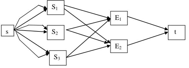
Consider a workshop having two similar lathes E1 and E2 which are being used for manufacturing three types of roller sets S1, S2 and S3. Assume that both the lathes are capable of manufacturing any of the products and the capacity of each of the lathes (Akr) is 400 units for each of the product with the yield rates to be 85%. Consider the order position for priority orders and normal orders for the three roller sets S1, S2 and S3 to be as shown in Table 1.

Note that changeover for handling one type of roller to the other type incurs certain time and associated costs. Since the changeover costs increase with the number of set ups, to minimize the costs associated with the set ups, similar types of products should be processed successively so that the total number of changeovers are minimized. This problem is equivalent to the problem of maximizing the total capacity utilization. This example illustrates the steps in scheduling the workshop.

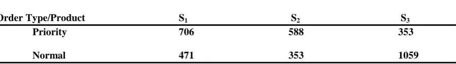
Table 1: Order position and priorities for Example 1

Order Type/Product S1 S2 S3

Priority 600 500 300

Normal 400 300 900

The PROCESSNET for the workshop is as shown in Figure 1.

Figure 1: PROCESSNET for the Workshop of Example 1.

Step 1:Consider the PROCESSNET with single directed arcs (with arc number i=1).

The demand Dki for the product Sk by Order type i will be as follows: D11=600, D12=400, D21=500, D22=300, D31=300 and D32=900.

The yield adjusted order quantity Dki/gk (rounded integer) for the product Sk by the customer Ci, with priority i is given in Table 2.

s

S

1

111

1

S

2

111

1 S

1 ₃

111

1

E

1

111

1

E

2

111

1

t

111

(4)

Table2. Yield adjusted order position and delivery schedules for the two customers C1 and C2

Priority 706 588 353

Normal 471 353 1059

The capacity along the arc from s to Sk (k=1,2,3) is the yield adjusted order quantity Dki for the product Sk by the order type i=1, viz., D11=706, D21=588, and D31=353 respectively. The capacity of the arc (Sk, Er) is considered as Akr which is the capacity of processing product Sk by equipment Er. The capacities of the arcs (Er,t) are considered as infinity (in this example, it is considered as 10000000).

The excel formulation of the problem is shown in Table 3.

Table 3: Excel formulation of Step 1 of Example 1

From To Flow Capacity Nodes Net Flow Supply/Demand s s1 0 <= 706 s 0

s s2 0 <= 588 s1 0 = 0

s s3 0 <= 353 s2 0 = 0

s1 E1 0 <= 400 s3 0 = 0

s1 E2 0 <= 400 E1 0 = 0

s2 E1 0 <= 400 E2 0 = 0

s2 E2 0 <= 400 t 0 s3 E1 0 <= 400 s3 E2 0 <= 400 E1 t 0 <= 10000000 E2 t 0 <= 10000000 Max.

Flow 0

Using excel solver, the maximal flow as shown in Table 4 is obtained.

Table 4: Solver solution of Step 1 of Example 1. Variable Cells

Cell Name

Original

Value Final Value

$D$4 s1 Flow 0 706

$D$5 s2 Flow 0 588

$D$6 s3 Flow 0 353

$D$7 E1 Flow 0 400

$D$8 E2 Flow 0 306

$D$9 E1 Flow 0 400

$D$10 E2 Flow 0 188

(5)

$D$12 E2 Flow 0 353

$D$13 t Flow 0 800

$D$14 t Flow 0 847

Step 2:Consider the same PROCESSNET with single directed arcs (with arc number i=2)

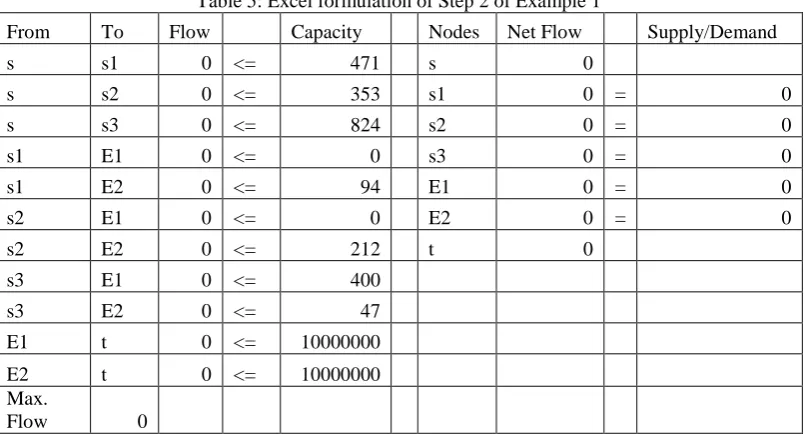
The capacity along the arc from s to Sk (k=1,2,3) is the the yield adjusted order quantity Dki for the product Sk by the order type i=2, viz., D12=471, D22=353, and D32=1059 respectively. The capacity of the arc (Sk, Er) is considered as Min.[Akr , Akr – optimum flow along (Sk,Er) in Step1]. For example, capacity of the arc (S1, E1) is Min.[400, 400-400]=0. The capacities of the arcs (Er,t) are considered as infinity (in this example, it is considered as 10000000).

The excel formulation of the problem is shown in Table 5.

Table 5: Excel formulation of Step 2 of Example 1

From To Flow Capacity Nodes Net Flow Supply/Demand s s1 0 <= 471 s 0

s s2 0 <= 353 s1 0 = 0

s s3 0 <= 824 s2 0 = 0

s1 E1 0 <= 0 s3 0 = 0

s1 E2 0 <= 94 E1 0 = 0

s2 E1 0 <= 0 E2 0 = 0

s2 E2 0 <= 212 t 0 s3 E1 0 <= 400 s3 E2 0 <= 47 E1 t 0 <= 10000000 E2 t 0 <= 10000000 Max.

Flow 0

Using excel solver, the following maximal flow as shown in Table 6 is obtained.

Table 6: Solver solution of Step 2 of Example 1 Variable Cells

Cell Name Original Value Final Value

$D$4 s1 Flow 0 94

$D$5 s2 Flow 0 212

$D$6 s3 Flow 0 447

$D$7 E1 Flow 0 0

$D$8 E2 Flow 0 94

$D$9 E1 Flow 0 0

$D$10 E2 Flow 0 212

$D$11 E1 Flow 0 400

$D$12 E2 Flow 0 47

$D$13 t Flow 0 400

(6)

The optimal scheduling is obtained by considering the optimal flows obtained in Step 1 and Step 2, which can be represented as in Table 7.

Table 7: Optimal scheduling for Example 1

Optimal Schedules Opt. Flow1 Opt.Flow2

Product s1 (Priority/Normal) 706 94

Machine 1 400 0

Machine 2 306 94

Machine 1 400 0

Machine 2 188 212

Machine 1 0 400

Machine 2 353 47

Machine 1 Total 800 400

The optimal flows along the arcs (s,Sk) provides the optimal scheduling for the lathes 1 and 2 and for the products 1,2 and 3 respectively. In other words, f* = (706, 94, 588, 212, 353, 447) for the arcs (s,Sk). The yield adjusted optimal supplies to the customers will be f* = (600, 80, 500, 180, 300, 380)

Thus, the optimal quantities to be supplied to the priority and normal customers and the corresponding unfulfilled demands (as shown in the brackets) are as in Table 8. Observe that there are 200 units each of unfulfilled quantities for normal customer for the products S1 and S3. These quantities could be rescheduled with customer's concurrence.

Table 8: Optimal supply quantities and the unfulfilled demands

Priority 600 500 300

(0) (0) (0)

Normal 80 180 380

(320) (120) (520)

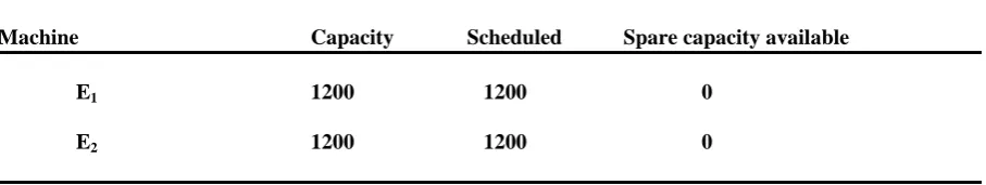
The capacities, scheduled/utilized capacities and the corresponding spare capacity available for the two lathes are shown in Table 9.

Table 9: Machine utilization and the spare capacities available for Example 1

Machine Capacity Scheduled Spare capacity available

E1 1200 1200 0

E2 1200 1200 0

(7)

It can be observed that, if the capacity exceeds the scheduled quantity, the difference provides the available spare capacity for each machine.

Example 2: 3 Machines and 5 Products (Scheduling when order books are not full)

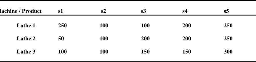
Consider a workshop having three lathes E1, E2 and E3 which are being used for manufacturing five types of roller sets S1 to S5. Let the machine capacities be as in Table 10 and the yield rates be 85%.

Table 10: Machine capacities for lathes in Example 2

Machine / Product s1 s2 s3 s4 s5

Lathe 1 250 100 100 200 250

Lathe 2 50 100 200 200 250

Lathe 3 100 100 150 150 300

Consider the order position for priority orders and normal orders for the five roller sets S1 to S5 to be as shown in Table 11.

Table 11: Order position and priorities for Example 2

Order Type/Product s1 s2 s3 s4 s5 Priority 200 100 50 300 150

Normal 100 200 150 50 400

The yield adjusted order quantity Dki/gk (rounded integer) for the product Sk by the customer Ci, with priority i is given in Table 12.

Table 12: Yield adjusted order position and priorities for Example 2.

Order Type/Product s1 s2 s3 s4 s5 Priority 235 118 59 353 176

Normal 118 235 176 59 471

(8)

Table 13: Optimal scheduling for Example 2.

Optimal Schedules Opt. Flow1 Opt.Flow2

Machine 1 135 115

Machine 2 0 3

Machine 3 100 0

Machine 1 100 88

Machine 2 18 47

Machine 3 0 100

Machine 1 59 85

Machine 2 0 91

Machine 3 0 0

Machine 1 3 59

Machine 2 200 0

Machine 3 150 0

Machine 1 0 97

Machine 2 0 250

Machine 3 176 124

The optimal flows along the arcs (s,Sk) provides the optimal scheduling for the lathes 1,2 and 3 and for the products 1 to 5 respectively. In other words, f* = (235, 118, 118, 235, 59, 176, 353, 59, 176, 471) for the arcs (s,Sk). The yield adjusted optimal supplies to the customers will be f* = (200, 100, 100, 200, 50, 150, 300, 50, 150, 400) for the arcs (s,Sk).

Thus, the optimal quantities to be supplied to the priority and normal customers satisfy the ordered quantities, as shown in Table 11.

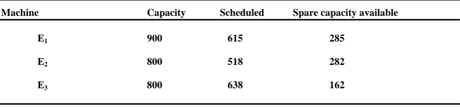
The capacities, scheduled/utilized capacities and the corresponding spare capacity available for the three machines are shown in Table 14.

Table 14: Equipment utilization and the spare capacities available for Example 2

Machine Capacity Scheduled Spare capacity available

E1 900 615 285

E2 800 518 282

E3 800 638 162

(9)

4. Conclusion

In this paper, a working implementation of the excel solver for scheduling the MAN with gains, developed by Bokkasam (2018), is presented. The excel has been validated with results obtained and we can now solve large problems involving many machines and products. The methodology of the system described above is in general applicable to all single-stage, multi-item compatible production processes where the process can handle different types of products. This methodology takes into account the yield for the product as well, which reflects the actual quantity of material delivered to the customer and can be compared with the order quantity. Depending on the layout and process flow of the plant, a tailor-made production planning and scheduling system can be formulated using the suitable MAN with gains model and the excel solver application. In future, the managers will be able to use this technique for obtaining the results immediately for scaled-up scenarios.

References

[1]. Akturk, M. S., S. Ozkan, 2001. Integrated Scheduling and Tool Management in Flexible Manufacturing Systems. International Journal of Production Research. 39(12), 2697-2722.

[2]. Bokkasam Sasidhar, 2016. Multiple Arc Network Model for Scheduling in a Single-stage, Multi-item Compatible Process, International Review of Management and Business Research. 5(3), 1223-1231. [3]. Bokkasam Sasidhar, 2018. Scheduling in a Single-stage, Multi-item Compatible Process using Multiple

Arc Network with Gains Model, International Journal of Research in Business Studies and Management. 5(9), 15-20.

[4]. Burkard, R. E. and Hatzl, J., 2005. Review, Extensions and Computational Comparison of MILP Formulations for Scheduling of Batch Processes, Comput. Chem. Eng. 29, 1752–1769.

[5]. Daniel Fylstra, Leon Lasdon, John Watson and Allan Waren, 1998. Design and Use of the Microsoft Excel Solver, INTERFACES. 28(5), 29-55.

[6]. Daniela Borissova, 2008. Optimal Scheduling for Dependent Details Processing Using MS Excel Solver. Cybernetics and Information Technologies. 8(2), 102-111.

[7]. Erik Prada, Alena Pešková, Michael Valášek, 2015. Model of Maintenance Planning Based on Trend of Machines Failures with Two Priorities, World Journal of Engineering and Technology. 3, 205-210. [8]. Eugénio C. Ferreira and Romualdo Salcedo., 2001. Can spreadsheet solvers solve demanding

optimization problems? Computer Applications in Engineering Education. 9, 49–56.

[9]. Floudas, C. A. and Lin, X., 2004. Continuous-Time versus Discrete-Time Approaches for Scheduling of Chemical Processes: A Review, Comput. Chem. Eng. 28, 2109–2129.

[10]. Ford, L.R. and Fulkerson, D.R., 2010. Flows in Networks, Princeton University Press, Princeton, NJ. [11]. Geoffrion, A. M., 1991. Forces, trends, and opportunities in Management Science and Operations

Research, Operations Research. 4(3), 423-445.

[12]. J. Duda, A. Stawowy, R. Basiura, 2014. Mathematical Programming for Lot Sizing and Production Scheduling in Foundries. Archives of Foundry Engineering. 14(3), 17-20.

[13]. Kallrath, J., 2002. Planning and Scheduling in the Process Industry, OR Spectrum. 24, 219–250 [14]. Mendez C. A., Cerda´J., Grossmann I. E., Harjunkoski I. and Fahl, M., 2006. State of-the-Art Review

of Optimization Methods for Short-Term Scheduling of Batch Processes, Comput. Chem. Eng. 30, 913–946.

[15]. Morton, T. E., D. W. Pentico, 1993. Heuristic Scheduling Systems with Applications to Production Systems and Project Management. New York, Wiley.

[16]. Pan M., Li X. and Qian, Y., 2009. Continuous-Time Approaches for Short-Term Scheduling of Network Batch Processes: Small-Scale and Medium-Scale Problems, Chem. Eng. Res. Des. 87, 1037– 1058.

[17]. Pinto, J. M. and Grossmann, I. E., 1998. Assignment & Sequencing Models for the Scheduling of Process Systems, Ann. Oper. Res. 81, 433–466.

[18]. Rita Kumar, 2017. A Spreadsheet-based Scheduling Model to Create Individual Graduation Roadmaps, Journal of Supply Chain and Operations Management. 15(2),165-188.

[19]. Saksena, J.P., 1982. Applications of O.R. Techniques -3. Decision Networks with Managerial Applications, National Productivity Council, New Delhi, India.

(10)

[21]. Sasidhar, B. and Achary, K.K., 1991. A multiple arc network model of production planning in a steel mill, International Journal of Production Economics. 22, 195-202.

[22]. Sun, J., D. Xue, 2001. A Dynamic Reactive Scheduling Mechanism for Responding to Changes of Production Orders and Manufacturing Resources, Computers in Industry. 46(2), 189-207.

[23]. Thomas T. Amlie., 2009. Constrained Optimization Problems in Cost And Managerial Accounting – Spreadsheet Tools, American Journal of Business Education. 2(6), 11-22.