Variational and convex approximations of 1-dimensional optimal networks and hyperbolic obstacle problems

(1)

Doctoral School in Mathematics

Variational and convex approximations of 1-dimensional

optimal networks and hyperbolic obstacle problems

Mauro Bonafini

UNIVERSIT `A DEGLI STUDI DI TRENTO

Dipartimento di Matematica

UNIVERSIT `A DEGLI STUDI DI VERONA

Dipartimento di Informatica

(2)

(3)

Doctoral thesis in Mathematics

Joint doctoral programme in Mathematics, XXXI cycle. Department of Mathematics,

University of Trento.

Department of Computer Science, University of Verona.

(4)

(5)

Introduction

In this thesis we investigate variational problems involving 1-dimensional sets (e.g., curves, networks) and variational inequalities related to obstacle-type dynamics from a twofold prospective. On one side, we provide variational approximations and convex relax-ations of the relevant energies and dynamics, moving mainly within the framework of Γ-convergence and of convex analysis. On the other side, we thoroughly investigate the numerical optimization of the corresponding approximating energies, both to recover op-timal 1-dimensional structures and to accurately simulate the actual dynamics.

Variational approximations and convex relaxation to the Gilbert–Steiner problem.

The starting point of our research is the Steiner tree problem: givenN distinct terminal points P1, . . . , PN in the Euclidean space Rd, find the shortest connected graph joining

them. In a more abstract way, what we are looking for is a minimizer of

(STP) inf{H1(L),L connected, {P1, . . . , PN} ⊂L}.

It is well known that an optimizer L for (STP) always exists, the solution being, in general, not unique for symmetric configurations of the terminal points. Any optimizer L turns out to be a tree, called Steiner Minimal Tree (SMT), and can be described as a union of segments connecting the given points, possibly meeting at 120◦in at mostN−2 further branched points, called Steiner points.

From a computational point of view, finding an SMT is known to be an NP-hard problem, even NP complete in certain cases: taking into account the upper bound on the number of possible Steiner points, the real problem, and thus the source of the high combinatorial complexity, is indeed to sort out the topology of an optimal graph. Many different approaches have been proposed to tackle the problem from a discrete point of view, both looking for exact algorithms in dimension 2 and 3 [110, 54] and providing more general PTAS approximation schemes [13, 14]. These algorithms are, up to date, the most efficient way to compute exact or approximated solutions to (STP), and it is not our purpose to battle in efficiency with them. Instead, we would like to look at the problem from the point of view of the Calculus of Variations, in order to provide a more robust variational approach to (STP) and, more generally, to problems involving 1-dimensional sets.

(6)

inRd, we look for the optimal way to transportN−1 unit masses located atP1, . . . , PN−1 toPN. Such a transportation is realized through a graphL=∪Ni=1−1λi, where eachλi is a

simple rectifiable curve that connects Pi toPN and represents the path of the ith mass.

Taking into account scaling effects, i.e., the more we transport the less we pay per unit mass, we fix 0≤α≤1 and look for an optimizer of

(Iα) inf

( Z

L

|θ(x)|αdH1(x), θ(x) =

N−1 X

i=1

1λi(x)

) .

The fact that θ(x) 7→ |θ(x)|α _{is a sublinear concave function of the transported mass}

densityθ enforces aggregation of masses and the emergence of branching structures [21]. We notice that (I1) corresponds to the Monge optimal transport problem, while (I0) corresponds to (STP). As for (STP) a solution to (Iα) is known to exist and any optimal

network turns out to be a tree.

In the recent years, as we outline in 1.1, many variational approaches for (Iα) have

been proposed. Among them, the stepping stone of this thesis is the interpretation of (Iα) as a mass minimization problem in a cobordism class of integral currents with

multiplicities in a suitable normed group as studied by Marchese and Massaccesi in [70, 69]. The underlying idea is to switch our focus from a problem involving families ofN−1 curves{λ1, . . . , λN−1} each one connecting Pi to PN, to a problem involving families of

integral rectifiable 1-currents Λ = (Λ1, . . . ,ΛN−1) ∈[I1(Rd)]N−1 where each component

has boundary ∂Λi =δPN −δPi. Within such a framework, given a norm Ψ onR

N−1_{, we} introduce the Ψ-mass of Λ∈[I1(Rd)]N−1 as

||Λ||_Ψ:= sup

ω∈Cc∞(Rd;Rd)

h∈Cc∞(Rd;RN−1)

(_N₋₁ X

i=1

Λi(hiω), |ω(x)| ≤1,Ψ∗(h(x))≤1

)

where Ψ∗ is the dual norm to Ψ with respect to the scalar product on RN−1. When one

chooses Ψ = Ψα as the`1/α-norm, it can be shown that (Iα) is equivalent to

(I_αc) inf{||Λ||_Ψ_α : Λ = (Λ1, . . . ,ΛN−1)∈[I1(Rd)]N−1, ∂Λi =δPN −δPi}.

The equivalence, as we are going to discuss in the forthcoming chapters, is meant in the sense that any minimizerLof (Iα) describes a minimizer ΛLof (Iαc) with the same energy

and, vice versa, the support of any minimizer of (I_αc) describes a minimal graph for (Iα).

Moving from this equivalence, the first three chapters of this thesis focus on Ψ-mass minimization problems among suitably defined families of integral rectifiable 1-currents (or, equivalently, rectifiable vector valued measures), where Ψ is chosen in order to re-produce the desired behaviour of the optimal structures we are looking for. As our main results we provide a variational approximation of Ψ-mass minimization problems in Rd

for any dimension d≥2 and we introduce a suitable notion of convex relaxation for (Iα)

(7)

restriction of (I_αc) will be essential for the derivation of a sharp relaxed energy. The first three chapters are organized as follows.

Variational approximation in the planar case. In Chapter 1 we mainly focus on the planar caseR2, where a Ψ-mass minimization problem can be further recast in terms of an

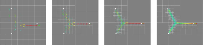
optimal partition type problem involving integer valued vector functions. We provide a variational approximation of the arising limiting functional by means of Modica–Mortola type energies, and we prove that minimizers of regularized functionals identify, in the limit, a (local) minimizer of (Iα). We therefore address the numerical optimization of

these regularized energies and provide examples for variousαand different configurations of the endpoints. The content of Chapter 1 represents a joint work with G. Orlandi and ´E. Oudet, published in “SIAM Journal on Mathematical Analysis” [25]. The same results were previously announced in “Geometric Flows” [22] and in “Rendiconti Lincei - Matematica e Applicazioni” [24].

Variational approximation in arbitrary dimension. In Chapter 2 we switch our focus on the higher dimensional scenario, and provide a variational approximation of Ψ-mass energies by means of Ginzburg–Landau type functionals. The results build upon the work presented in [5, 6] and use as main technical tool the relationship between boundaries and Jacobians of vector valued Sobolev maps. The content of Chapter 2 represents a joint work with G. Orlandi and ´E. Oudet, currently submitted for publication [26].

Convex relaxation. One of the main issues in the direct numerical optimization of Ψα-mass problems in the form of (Iαc) resides in the non convexity of the set of candidate

minimizers, which are generally only rectifiable objects with integer multiplicities. In Sec-tion 1.4, to overcome this issue, we investigate possible convex relaxaSec-tions of the problem, much in the spirit of [43]. We look at convex extensions of the energy on a wider class of objects, so as to include in the picture also diffused objects with real valued multiplicities. The sharpest of these relaxations is the main subject of Chapter 3, where we present an extensive numerical investigation of it both in two and three space dimensions. Further-more, we propose to extend this convex framework to more generalα-irrigation problems (with multiple sources/sinks) and to use the same approach to address Gilbert–Steiner problems on manifolds. The main advantage of the proposed framework relies in the possibility to introduce a corresponding notion of calibration, giving us an analytical tool to prove that minimizers of the relaxed functional are convex combinations of minimizers of (Iα). However, as discussed in Chapter 3, there exist configurations of the endpoints

for which the relaxation fails to recover convex combinations of minimal graphs, proving in turn that for these configurations optima of (Iα) cannot be calibrated. The content

of Chapter 3 represents a joint work with ´E. Oudet, currently submitted for publication [27] and partly announced in [22].

Hyperbolic obstacle problems.

(8)

time that the solution must lie above a given “obstacle”g. In case of an evolutive equation, one can think of the obstacleg as a physical obstruction to the movement. Consider, for example, the dynamic of a string having fixed extrema and oscillating above a table: as soon as the string reaches the table we have to take into account the collision, and such an interaction cannot be described by a classical PDE, but it is rather described by a variational inequality [107, 55].

Obstacle problems for the minimizers of classical energies and regularity of the arising free boundary have been extensively studied in the literature, together with the corre-sponding evolutive equations in a parabolic context (cf. Section 4.1). What seems to be missing in the picture is the hyperbolic scenario which, despite being in some cases as natural as the previous ones, has received little attention so far. In Chapter 4 we study the obstacle problem for the fractional wave equation

utt+ (−∆)su= 0

where (−∆)s _{is the fractional Laplace operator of exponent} _s_{, with} _{s >}_{0. For suitable}

initial data at timet= 0, we study the problem assuming homogeneous Dirichlet bound-ary conditions and under the additional constraintu≥gfor a given profileg. The idea is to apply a convex minimization approach based on a semi-discrete approximation scheme: at each time step the subsequent approximation in time is obtained as the unique opti-mizer of a suitably defined convex energy depending on previous steps. Such an approach has been extensively exploited in the literature to address parabolic and hyperbolic evo-lution problems, and fits within the general framework of minimizing movements. As main result we prove existence of a suitably defined weak solution, together with the corresponding energy estimates. The approximating scheme allows to perform numerical simulations which give quite precise evidence of dynamical effects. In particular, based on our numerical experiments, we conjecture that this method is able to select, in cases of non uniqueness, the most dissipative solution, that is to say the one losing the maximum amount of energy at contact times. The content of Chapter 4 represents a joint work with M. Novaga and G. Orlandi, currently submitted for publication [23].

Summary of research outcome.

The thesis work led to the following publications and preprints, some of which constitute the content of this manuscript.

[22] Mauro Bonafini. Convex relaxation and variational approximation of the Steiner problem: theory and numerics. Geom. Flows, 3:19–27, 2018

[23] Mauro Bonafini, Matteo Novaga, and Giandomenico Orlandi. A variational scheme for hyperbolic obstacle problems.Submitted, arXiv preprint arXiv:1901.06974, 2019

(9)

[25] Mauro Bonafini, Giandomenico Orlandi, and ´Edouard Oudet. Variational approx-imation of functionals defined on 1-dimensional connected sets: the planar case.

SIAM J. Math. Anal., 50(6):6307–6332, 2018

[26] Mauro Bonafini, Giandomenico Orlandi, and ´Edouard Oudet. Variational approx-imation of functionals defined on 1-dimensional connected sets in Rn. Submitted,

2019

(10)

(11)

Chapter 1

Variational approximation of

functionals defined on

1-dimensional connected sets: the

planar case

In this chapter we consider variational problems involving 1-dimensional connected sets in the Euclidean plane, such as the classical Steiner tree problem and the irrigation (Gilbert– Steiner) problem. We relate them to optimal partition problems and provide a variational approximation through Modica–Mortola type energies proving a Γ-convergence result. We also introduce a suitable convex relaxation and develop the corresponding numerical implementations. The proposed methods are quite general and the results we obtain can be extended to n-dimensional Euclidean space as shown in the next chapter.

1.1

Introduction

(14)

The Steiner Tree Problem (STP) [58] can be described as follows: given N points P1, . . . , PN in a metric space X (e.g., X a graph, with Pi assigned vertices) find a

con-nected graph F ⊂ X containing the points Pi and having minimal length. Such an

optimal graphF turns out to be a tree and is thus called aSteiner Minimal Tree (SMT). In case X = Rd, d ≥ 2 endowed with the Euclidean `2 metric, one refers often to the

EuclideanorgeometricSTP, while forX=Rdendowed with the`1 (Manhattan) distance

or forX contained in a fixed grid G ⊂_Rd _{one refers to the} _rectilinear_{STP. Here we will}

adopt the general metric space formulation of [86]: given a metric spaceX, and given a compact (possibly infinite) set of terminal pointsA⊂X , find

(STP) inf{H1(S),S connected, S⊃A},

whereH1 _{indicates the 1-dimensional Hausdorff measure on}_X_{. Existence of solutions for} (STP) relies on Golab’s compactness theorem for compact connected sets, and it holds true also in generalized cases (e.g., infH1₍_S_),_S_∪_A_connected).

The Gilbert–Steiner problem, or α-irrigation problem [21, 112] consists of finding a network S along which to flow unit masses located at the sources P1, . . . , PN−1 to the target point PN. Such a network S can be viewed as S = ∪_iN₌₁−1γi, with γi a path

connecting Pi toPN, corresponding to the trajectory of the unit mass located atPi. To

favour branching, one is led to consider a cost to be minimized byS which is a sublinear (concave) function of the mass density θ(x) =PN−1

i=1 1γi(x): i.e., for 0≤α≤1, find

(Iα) inf

Z

S

|θ(x)|αdH1(x).

Notice that (I1) corresponds to the Monge optimal transport problem, while (I0) cor-responds to (STP). As for (STP) a solution to (Iα) is known to exist and the optimal

networkS turns out to be a tree [21].

Problems like (STP) or (Iα) are relevant for the design of optimal transport channels

or networks connecting given endpoints, for example, the optimal design of net routing in VLSI circuits in the case d= 2,3. The Steiner Tree Problem has been widely studied from the theoretical and numerical point of view in order to efficiently devise constructive solutions, mainly through combinatoric optimization techniques. Finding a Steiner Min-imal Tree is known to be a NP hard problem (and even NP complete in certain cases), see, for instance, [13, 14] for a comprehensive survey on PTAS algorithms for (STP).

The situation in the Euclidean case for (STP) is theoretically well understood: given N points Pi ∈ Rd a SMT connecting them always exists, the solution being in general

not unique (think, for instance, to symmetric configurations of the endpoints Pi). The

SMT is a union of segments connecting the endpoints, possibly meeting at 120◦ in at mostN−2 further branch points, called Steiner points.

Nonetheless, the quest of computationally tractable approximating schemes for (STP) and for (Iα) has recently attracted a lot of attention in the Calculus of Variations

commu-nity. In particular, (Iα) has been studied in the framework of optimal branched transport

(15)

problem for 1-dimensional connected sets [77, 49], or even a Plateau problem in a suit-able class of vector distributions endowed with some algebraic structure [77, 70], to be solved by finding suitable calibrations [74]. Several authors have proposed different ap-proximations of those problems, whose validity is essentially limited to the planar case, mainly using a phase field based approach together with some coercive regularization, see, e.g., [30, 44, 82, 29].

Our aim is to propose a variational approximation for (STP) and for the Gilbert– Steiner irrigation problem (in the equivalent formulations of [112, 69]) in the Euclidean case X = Rd, d ≥ 2. In this chapter we focus on the planar case d = 2 and prove a

Γ-convergence result (see Theorem 1.3.12 and Proposition 1.3.11) by considering integral functionals of Modica–Mortola type [76]. In Chapter 2 we rigorously prove that certain integral functionals of Ginzburg-Landau type (see [6]) yield a variational approximation for (STP) and (Iα) valid in any dimension d ≥ 3. This approach is related to the

interpretation of (STP) and (Iα) as a mass minimization problem in a cobordism class of

integral currents with multiplicities in a suitable normed group as studied by Marchese and Massaccesi in [70, 69] (see also [77] for the planar case). Our method is quite general and may be easily adapted to a variety of situations (e.g., in manifolds or more general metric space ambients, with densities or anisotropic norms, etc.).

The plan of the chapter is as follows: in Section 1.2 we reformulate (STP) and (Iα) as

a suitable modification of the optimal partition problem in the planar case. In Section 1.3, we state and prove our main Γ-convergence results, respectively Proposition 1.3.11 and Theorem 1.3.12. Inspired by [43], we introduce in Section 1.4 a convex relaxation of the corresponding energies. In Section 1.5 we present our approximating scheme for (STP) and for the Gilbert-Steiner problem and illustrate its flexibility in different situations, showing how our convex formulation is able to recover multiple solutions whereas Γ-relaxation detects any locally minimizing configuration.

1.2

Steiner problem for Euclidean graphs and optimal

par-titions

In this section we describe some optimization problems on Euclidean graphs with fixed endpoints setA, like (STP) or irrigation-type problems, following the approach of [70, 69], and we rephrase them as optimal partition-type problems in the planar case R2.

1.2.1 Rank one tensor valued measures and acyclic graphs

For M > 0, we consider Radon measures Λ on Rd with values in the space of matrices Rd×M. For each i = 1, . . . , M we define as Λi the vector measure representing the ith

column of Λ, so that we can write Λ = (Λ1, . . . ,ΛM). The total variation measures |Λi|

are defined as usual with respect to the Euclidean structure on Rd, while we set µΛ = PM

(16)

and i= 1, . . . , M, such that Λ =p(x)µΛ and PM_i₌₁|pi(x)|= 1 for µΛ-a.e x∈Rd (where

on vectors of Rd | · | denotes the Euclidean norm). Whenever p is a rank one matrix

µΛ-almost everywhere we say that Λ is a rank one tensor valued measure and we write it as Λ =τ⊗g·µΛfor aµΛ-measurable unit vector fieldτ inRdandg:Rd→RM satisfying

PM

i=1|gi|= 1.

Given Λ∈ M(Rd,Rd×M) and a function ϕ∈Cc∞(Rd;Rd×M), withϕ= (ϕ1, . . . , ϕM),

we have

hΛ, ϕi=

M

X

i=1

hΛ_i, ϕii= M

X

i=1 Z

Rd

ϕidΛi,

and fixing a norm Ψ onRM, one may define the Ψ-mass measure of Λ as

|Λ|_Ψ(B) := sup

ω∈C∞

c (B;Rd)

h∈C∞

c (B;RM)

{hΛ, ω⊗hi, |ω(x)| ≤1, Ψ∗(h(x))≤1} , (1.2.1)

forB ⊂_Rd_{open, where Ψ}∗ _{is the dual norm to Ψ w.r.t. the scalar product on}

RM, i.e.,

Ψ∗(y) = sup

x∈RM

hy, xi −Ψ(x).

Denote ||Λ||_Ψ = |Λ|_Ψ(Rd) the Ψ-mass norm of Λ. In particular, one can see that µΛ coincides with the measure |Λ|_`1, which from now on will be denoted as |Λ|1, and any

rank one measure Λ may be written as Λ =τ⊗g· |Λ|1so that|Λ|Ψ= Ψ(g)|Λ|1. Along the lines of [70] we will rephrase the Steiner and Gilbert–Steiner problem as the optimization of a suitable Ψ-mass norm over a given class of rank one tensor valued measures.

Let A={P1, . . . , PN} ⊂Rd,d≥2, be a given set of N distinct points, with N >2.

We define the class G(A) as the set of acyclic graphs L connecting the endpoints set A such that L can be described as the union L =∪N_i₌₁−1λi, where λi are simple rectifiable

curves with finite length having Pi as initial point and PN as final point, oriented by

H1_{-measurable unit vector fields}_τ

i satisfying τi(x) =τj(x) forH1-a.e. x∈ λi∩λj (i.e.,

the orientation ofλi is coherent with that of λj on their intersection).

For L∈ G(A), if we identify the curves λi with the vector measures Λi =τi· H1 λi,

all the information concerning this acyclic graph L is encoded in the rank one tensor valued measure Λ =τ⊗g· H1 _L_{, where the}_H1_{-measurable vector field} _τ _∈

Rd carrying

the orientation of the graph L satisfies sptτ = L, |τ| = 1, τ = τi H1-a.e. on λi, and

theH1_{-measurable vector map}_g_:

Rd→RN−1 has components gi satisfyinggi· H1 L=

H1 _λ

i=|Λi|, with|Λi|the total variation measure of the vector measure Λi =τ·H1 λi.

Observe that gi ∈ {0,1} a.e. for any 1≤i≤N −1 and, moreover, that each Λi verifies

the property

div Λi =δPi−δPN. (1.2.2)

Definition 1.2.1. Given any graph L∈ G(A), we call the above constructed ΛL ≡Λ =

τ⊗g · H1 _L _{the canonical rank one tensor valued measure representation of the acyclic}

(17)

To any compact connected set K ⊃ A with H1₍_K₎ _< _{+∞, i.e., to any candidate} minimizer for (STP), we may associate in a canonical way an acyclic graph L ∈ G(A) connecting {P1, . . . , PN} such thatH1(L)≤ H1(K) (see, e.g., Lemma 2.1 in [70]). Given

such a graph L ∈ G(A) canonically represented by the tensor valued measure Λ, the measure H1 _L_{corresponds to the smallest positive measure dominating}_H1 _λ

i for 1≤

i ≤ N −1. It is thus given by H1 _L _{= sup}

iH1 λi = supi|Λi|, the supremum of the

total variation measures|Λ_i|. We recall that, for any nonnegativeψ∈C_c0(Rd), we have

Z

Rd

ψ d

sup

i

|Λi|

= sup

(_N₋₁ X

i=1 Z

Rd

ϕid|Λi|, ϕi∈Cc0(Rd), N−1

X

i=1

ϕi(x)≤ψ(x)

) .

Remark 1.2.2 (graphs as G-currents). In [70], the rank one tensor measure Λ = τ ⊗g· H1 _L _{identifying a graph in}

Rd is defined as a current with coefficients in the group ZN−1 ⊂ RN−1. For ω ∈ D1(Rd) a smooth compactly supported differential 1-form and

~

ϕ= (ϕ1, ..., ϕN−1)∈[D(Rd)]N−1 a smooth test (vector) function, one sets

hΛ, ω⊗ϕ~i:= Z

Rd

hω⊗ϕ, τ~ ⊗gi dH1 L=

N−1 X

i=1 Z

Rd

hω, τiϕigidH1 L

=

N−1 X

i=1 Z

Rd

hω, τiϕid|Λi|.

Moreover, fixing a norm Ψ onRN−1, one may define the Ψ-mass of the current Λ as it is

done in (1.2.1). In [70] the authors show that classical integral currents, i.e., G=Z, are

not suited to describe (STP) as a mass minimization problem: for example, minimizers are not ensured to have connected support.

1.2.2 Irrigation-type functionals

In this section we consider functionals defined on acyclic graphs connecting a fixed set A={P1, . . . , PN} ⊂Rd,d≥2, by using their canonical representation as rank one tensor

valued measures, in order to identify the graph with an irrigation plan from the point sources{P1, . . . , PN−1}to the target pointPN. We focus here on suitable energies in order

to describe the irrigation problem and the Steiner tree problem in a common framework as in [70, 69]. We observe, moreover, that the irrigation problem with one point source (Iα) introduced by Xia [112], in the equivalent formulation of [69], approximates the

Steiner tree problem asα→0 in the sense of Γ-convergence (see Proposition 1.2.4). Consider on RN−1 the norms Ψα = | · |`1/α (for 0 < α ≤ 1) and Ψ₀ = | · |_`∞. Let Λ =τ ⊗g· H1 _L _{be the canonical representation of an acyclic graph} _L_{∈ G}₍_A_{), so that} we have|τ|= 1, gi ∈ {0,1} for 1≤i≤N −1 and hence |g|∞ = 1 H1-a.e. on L. Let us

define for such Λ and any α∈[0,1] the functional

Fα(Λ) :=||Λ||Ψα =|Λ|Ψα(R

(18)

Observe that, by (1.2.1),

F0(Λ) = Z

Rd

|τ||g|∞dH1 L=H1(L)

and

Fα_{(Λ) =}

Z

Rd

|τ||g|₁_/αdH1 _L₌ Z

L

|θ|α_d_H1_, _(1.2.3)

whereθ(x) =P

igi(x)1/α=

P

igi(x)∈Z, and 0≤θ(x)≤N−1. We thus recognize that

minimizing the functionalFα _{among graphs}_L_connecting _P

1, . . . , PN−1 toPN solves the

irrigation problem (Iα) with unit mass sources P1, . . . , PN−1 and target PN (see [69]),

while minimizing F0 _{among graphs} _L _{with endpoints set} _{_P

1, . . . , PN} solves (STP) in

Rd.

Since both Fα _and _F0 _{are mass-type functionals, minimizers do exist in the class of} rank one tensor valued measures. The fact that the minimization problem within the class of canonical tensor valued measures representing acyclic graphs has a solution in that class is a consequence of compactness properties of Lipschitz maps (more generally by compactness theorem forG-currents [70]; inR2it follows alternatively by the compactness

theorem in the SBV class [12]). Actually, existence of minimizers in the canonically oriented graph class inR2 can be deduced as a byproduct of our convergence result (see

Proposition 1.3.11 and Theorem 1.3.12) and inRd, ford >2, by the parallel Γ-convergence

analysis of Chapter 2.

Remark 1.2.3. A minimizer of F0 _(resp., _Fα_{) among tensor valued measures Λ}

repre-senting admissible graphs corresponds necessarily to the canonical representation of a minimal graph, i.e., gi ∈ {0,1} ∀1 ≤i≤N −1. Indeed since gi ∈Z, if gi 6= 0, we have

|gi| ≥1, hencegi∈ {−1,0,1}for minimizers. Moreover, if gi =−gj on a connected arc in

λi∩λj, withλi going fromPi toPN andλj going fromPj toPN, this implies thatλi∪λj

contains a cycle and Λ cannot be a minimizer. Hence, up to reversing the orientation of the graph,gi∈ {0,1}for all 1≤i≤N−1.

We conclude this section by observing in the following proposition that the Steiner tree problem can be seen as the limit of irrigation problems.

Proposition 1.2.4. The functional F0 _{is the} _Γ_{-limit, as} _α _→ ₀_{, of the functionals} _Fα

with respect to the convergence of measures.

Proof. Let Λ =τ⊗g·H1 _L_{be the canonical representation of an acyclic graph}_L_{∈ G(}_A_), so that |τ| = 1 and gi ∈ {0,1} for all i = 1, . . . , N −1. The functionals Fα(Λ) =

R

Rd|g|1/αdH

1 _L_{generates a monotonic decreasing sequence as}_α_→_{0, because}_|_g_|

p ≤ |g|q

for any 1 ≤ q < p ≤ +∞, and, moreover, Fα_(Λ) _{→ F}0_{(Λ) because} _|_g_|

q → |g|∞ as

q → +∞. Then, by elementary properties of Γ-convergence (see, for instance, Remark

1.40 of [33]) we haveFα ₋_{→ F}Γ 0 _.

(19)

1.2.3 Acyclic graphs and partitions of _R2

This section is dedicated to the two-dimensional case. The aim is to provide an equiv-alent formulation of (STP) and (Iα) in term of an optimal partition type problem. The

equivalence of (STP) with an optimal partition problem has been already studied in the caseP1, . . . , PN lie on the boundary of a convex set, see, for instance, [10, 11] and Remark

1.2.10.

To begin we state a result saying that two acyclic graphs having the same endpoints set give rise to a partition ofR2, in the sense that their oriented difference corresponds to the

orthogonal distributional gradient of a piecewise integer valued function having bounded total variation, which in turn determines the partition (see [12]). This is actually an instance of the constancy theorem for currents or the Poincar´e’s lemma for distributions (see [56]).

Lemma 1.2.5. Let {P, R} ⊂ R2 and let λ, γ be simple rectifiable curves from P to R

oriented by H1_{-measurable unit vector fields} _τ0_, _τ00_{. Define as above} _{Λ =}_τ0_{· H}1 _λ _and Γ =τ00· H1 _γ_.

Then there exists a function u ∈ SBV(R2;Z) such that, denoting Du and Du⊥

re-spectively the measures representing the gradient and the orthogonal gradient of u, we have Du⊥= Γ−Λ.

Proof. Consider simple oriented polygonal curves λk andγk connectingP toRsuch that

the Hausdorff distance to, respectively,λandγ is less than _k1 and the length ofλk (resp.,

γk) converges to the length ofλ(resp.,γ). We can also assume without loss of generality

that λk and γk intersect only transversally in a finite number of points mk ≥ 2. Let

τ_k0, τ_k00 be the H1_{-measurable unit vector fields orienting}_λ

k, γk and define the measures

Λk =τk0 · H1 λk and Γk=τk00· H1 γk.

For a given k ∈ N consider the closed polyhedral curve σk = λk∪γk oriented by

τk=τk0 −τk00 (i.e., we reverse the orientation ofγk). For everyx∈R2\σk let us consider

the index of x with respect toσk (or winding number) and denote it as

uk(x) = Indσk(x) =

1 2πi

I

σk

dz z−x.

By Theorem 10.10 in [95], the functionukis integer valued and constant in each connected

component of R2\σk and vanishes in the unbounded one. Furthermore, for a.e. x ∈σk

we have

lim

ε→0+uk(x+ετk(x)

⊥₎₋ _lim

ε→0−uk(x+ετk(x)

⊥_{) = 1}_,

i.e., uk has a jump of +1 whenever crossing σk from “right” to “left” (cf [91], Lemma

3.3.2). This means that

Du⊥_k =−τk· H1 σk= Γk−Λk.

Thus,|Duk|(R2) =H1(σk) andkukkL1₍

R2)≤C|Duk|(R

2_{) by Poincar´}_{e’s inequality in}_BV_. Hence uk ∈SBV(R2;Z) is an equibounded sequence in norm, and by Rellich

(20)

SBV(R2;Z). Taking into account that we haveDu⊥_k = Γk−Λk, we deduce, in particular,

thatDu⊥= Γ−Λ as desired.

Remark 1.2.6. Let A ⊂ _R2 _{as above. For} _i_{= 1}_{, ..., N} ₋_{1 let}_γ

i be the segment joining

Pi to PN, denote τi = _|P_PN−Pi

N−Pi| its orientation, and identify γi with the vector measure

Γi =τi· H1 γi. Then G =∪Ni=1−1γi is an acyclic graph connecting the endpoints set A

and H1₍_G_{) = (sup}

i|Γi|)(R2).

Given the set of terminal points A = {P1, . . . , PN} ⊂ R2 let us fix some G ∈ G(A)

(for example, the one constructed in Remark 1.2.6). For any acyclic graph L ∈ G(A), denoting Γ (resp., Λ) the canonical tensor valued representation ofG(resp.,L), by means of Lemma 1.2.5 we have

H1(L) = Z

R2

sup

i

|Λi|=

Z

R2

sup

i

|Du⊥_i −Γi| (1.2.4)

for suitable ui ∈ SBV(R2;Z), 1 ≤ i ≤ N −1. Thus, using the family of measures

Γ = (Γ1, . . . ,ΓN−1) of Remark 1.2.6, we are led to consider the minimization problem for

U ∈SBV(R2;ZN−1) for the functional

F0(U) =|DU⊥−Γ|Ψ0(R

2_{) =} Z

R2

sup

i

|Du⊥_i −Γi|. (1.2.5)

Proposition 1.2.7. There exists U ∈SBV(R2;ZN−1) such that

F0(U) = inf

V∈SBV(R2;ZN−1)

F0(V).

Moreover, sptU ⊂Ω ={x∈_R2 _: _|_x_|_<_{10 max}

i|Pi|}.

Proof. Observe first that for any U ∈ SBV(R2;ZN−1) with F0(U)<∞, we can find ˜U

s.t. F0( ˜U) ≤ F0(U) and spt ˜U ⊂ Ω. Indeed, consider r = 8 maxi|Pi|, χ = 1Br(0) and

˜

U = (χu1, . . . , χuN−1). One has, for 1≤i≤N −1, Z

R2\Br(0)

|Du˜i|=

Z

∂Br(0)

|u+_i |

whereu+_i is the trace on∂Br(0) ofui restricted to Br(0), and

Z

R2

|Du˜⊥_i −Γi|=

Z

Br(0)

|Du⊥_i −Γi|+

Z

∂Br(0)

|u+_i |

≤ Z

Br(0)

|Du⊥_i −Γi|+

Z

R2\Br(0)

|Dui|=

Z

R2

|Du⊥_i −Γi|

for any i= 1, . . . , N−1, i.e.,F0( ˜U)≤F0(U).

Now consider a minimizing sequence Uk ∈SBV(R2;ZN−1) of F0. We may suppose

w.l.o.g. spt(Uk)⊂Ω, so that, for any 1≤i≤N −1,

(21)

forksufficiently large. Hence Uk is uniformly bounded inBV by Poincar´e inequality on Ω, so that it is compact in L1_(Ω;

RN−1) and, up to a subsequence, Uk→U a.e., whence

U ∈SBV(Ω;ZN−1), sptU ⊂Ω andU minimizesF0 by lower semicontinuity of the norm.

We have already seen that to each acyclic graphL∈ G(A) we can associate a function U ∈ SBV(R2;ZN−1) such that H1(L) = F0(U). On the other hand, for minimizers of

F0_{, we have the following}

Proposition 1.2.8. Let U ∈ SBV(R2;ZN−1) be a minimizer of F0, then there exists

an acyclic graph L ∈ G(A) connecting the terminal points P1, . . . , PN and such that

F0(U) =H1₍_L₎_.

Proof. Let U = (u1, . . . , uN−1) be a minimizer of F0 in SBV(R2;ZN−1), and denote

Λi = Γi−Du⊥i . Observe that each Dui has no absolutely continuous part with respect

to the Lebesgue measure (indeed ui is piecewise constant being integer valued) and so

Λi =τi· H1 λi for some 1-rectifiable setλi and H1-measurable vector fieldτi. Since we

have div Λi =δPi−δPN, λi necessarily contains a simple rectifiable curve λ

0

i connecting

Pi toPN (use, for instance, the decomposition theorem for rectifiable 1-currents in cyclic

and acyclic part, as it is done in [69], or the Smirnov decomposition of solenoidal vector fields [106]).

Now consider the canonical rank one tensor measure Λ0 associated to the acyclic sub-graphL0 =λ0₁∪ · · · ∪λ0_N₋₁ connectingP1, . . . , PN−1 toPN. Then by Lemma 1.2.5, there

exists U0 = (u0₁, . . . , u0_N₋₁) ∈ SBV(R2;ZN−1) such that Du0i

⊥

= Γi−Λ0_i and in

partic-ularF0(U0) =H1₍_L0₎_{≤ H}1₍_L₎_≤_F0₍_U_{). We deduce}_H1₍_L0_{) =}_H1₍_L_{), hence}_L0 ₌_L_,_L_is

acyclic andH1₍_L_{) =}_F0₍_U_).

Remark 1.2.9. We have shown the relationship between (STP) and the minimization of F0 over functions in SBV(R2;ZN−1), namely

inf{F0(U) : U ∈SBV(R2;ZN−1)}= inf{F0(ΛL) : L∈ G({P1, . . . , PN})}.

A similar connection can be made between theα-irrigation problem (Iα) and minimization

overSBV(R2;ZN−1) of

Fα(U) =|DU⊥−Γ|_Ψ_α(R2), (1.2.6)

namely we have

inf{Fα(U) : U ∈SBV(R2;ZN−1)}= inf{Fα(ΛL) : L∈ G({P1, . . . , PN})},

whereFα _{is defined in equation (1.2.3). Indeed, given a norm Ψ on}

RN−1 andFΨ(U) =

|DU⊥−Γ|Ψ(R2) for U ∈ SBV(R2;ZN−1), the proofs of Propositions 1.2.7 and 1.2.8

carry over to this general context: there exists U ∈ SBV(R2;ZN−1) realizing infFΨ,

with sptU ⊂Ω andDU⊥−Γ = ΛLwith ΛL=τ⊗g· H1 Lthe canonical representation

(22)

Remark 1.2.10. In the case P1, . . . , PN ∈∂Ω with Ω⊂ R2 a convex set, we may choose

G=∪N_i₌₁−1γi withγi connectingPi toPN and sptγi ⊂∂Ω. We deduce by (1.2.4) that for

any acyclic graphL∈ G(A)

H1(L) = Z

Ω sup

i

|Du⊥_i |

for suitableui ∈SBV(Ω;Z) such that (in the trace sense) ui = 1 onγi ⊂∂Ω andui = 0

elsewhere in∂Ω, 1≤i≤N−1. We recover here an alternative formulation of the optimal partition problem in a convex planar set Ω as studied, for instance, in [10] and [11].

The aim of the next section is then to provide an approximation of minimizers of the functionalsFα (and more generallyFΨ) through minimizers of more regular energies of Modica–Mortola type.

1.3

Variational approximation of

F

α

In this section we state and prove our main results, namely Proposition 1.3.11 and The-orem 1.3.12, concerning the approximation of minimizers of Fα through minimizers of Modica–Mortola type functionals, in the spirit of Γ-convergence.

1.3.1 Modica–Mortola functionals for functions with prescribed jump

In this section we consider Modica–Mortola functionals for functions having a prescribed jump part along a fixed segment in R2 and we prove compactness and lower-bounds

for sequences having a uniform energy bound. Let P, Q ∈ _R2 _{and let} _s _{be the segment} connectingP toQ. We denote byτs= |QQ−−PP|its orientation and define Σs=τs·H1 s. Up

to rescaling, suppose max(|P|,|Q|) = 1 and let Ω =B10(0) and Ωδ= Ω\(Bδ(P)∪Bδ(Q))

for 0< δ |Q−P|. We consider the Modica–Mortola type functionals

Fε(u,Ωδ) =

Z

Ωδ

eε(u)dx=

Z

Ωδ

ε|Du⊥−Σs|2+

1

εW(u)dx, (1.3.1)

defined for u ∈Hs ={u ∈W1,2(Ωδ\s)∩SBV(Ωδ) : u|∂Ω = 0}, where W is a smooth non negative 1-periodic potential vanishing onZ(e.g.,W(u) = sin2(πu)). DefineH(t) =

2R₀tpW(τ)dτ and c0 =H(1).

Remark 1.3.1. Notice that any function u ∈ Hs with Fε(u,Ωδ) < ∞ has necessarily a

prescribed jumpu+−u−= +1 acrosss Ωδ in the direction νs=−τs⊥ in order to erase

the contribution of the measure term Σs in the energy. We thus have the decomposition

Du⊥ =∇u⊥L2₊_{J u}⊥₌_∇_u⊥_L2_{+ Σ}

s Ωδ,

where∇u∈L2(Ωδ) is the absolutely continuous part ofDuwith respect to the Lebesgue

measure L2_{, and} _{J u}_{= (}_u+₋_u−₎_ν

(23)

Remark 1.3.2. Notice that we cannot work directly in Ω with Fε due to summability

issues around the points P and Q for the absolutely continuous part of the gradient, indeed there are no functions u ∈ W1,2(Ω\s) such that u+−u− = 1 on s. To avoid this issue one could consider variants of the functionals Fε(·,Ω) by relying on suitable

smoothings Σs,ε = Σs∗ηε of the measure Σs, withηε a symmetric mollifier.

Proposition 1.3.3(Compactness). For any sequence{uε}ε ⊂Hs such thatFε(uε,Ωδ)≤

C, there existsu∈SBV(Ωδ;Z) such that (up to a subsequence)uε →u in L1(Ωδ).

Proof. By Remark 1.3.1 we haveDu⊥_ε =∇u⊥_εL2_+Σ

s Ωδ, and using the classical Modica–

Mortola trick one has

C≥ Z

Ωδ

ε|Du⊥_ε −Σs|2+

1

εW(uε)dx

= Z

Ωδ

ε|∇u⊥_ε|2+ 1

εW(uε)dx≥2 Z

Ωδ

p

W(uε)|∇uε|dx.

Recall that H(t) = 2R₀tpW(τ)dτ andc0=H(1). By the chain rule, we have

|D(H◦uε)|(Ωδ) = 2

Z

Ωδ

p

W(uε)|∇uε|dx+

Z

s

H(u+_ε)−H(u−_ε)

dH1(x)

≤C+c0H1(s).

We also have (H◦uε)|∂Ω= 0 sinceuεvanishes on∂Ω, so that, by the Poincar´e inequality,

{H◦uε}εis an equibounded sequence inBV(Ωδ), thus compact inL1(Ωδ). In particular,

there existsv∈L1(Ωδ) such that, up to a subsequence,H◦uε→vinL1(Ωδ) and pointwise

a.e. SinceH is a strictly increasing continuous function withc0(t−1)≤H(t)≤c0(t+ 1) for anyt∈_R, thenH−1 _{is uniformly continuous and}_|_H−1₍_t_{)| ≤}_c−1

0 (|t|+ 1) for allt∈R. Hence, up to a subsequence, the family {uε}ε ⊂L1(Ωδ) is pointwise convergent a.e. to

u = H−1(v) ∈ L1(Ωδ). By Egoroff’s Theorem, for any σ > 0 there exists a measurable

Eσ ⊂ Ωδ, with |Eσ| < σ, such that uε → u uniformly in Ωδ\Eσ. Then, taking into

account that |t| ≤c−₀1(|H(t)|+ 1) for allt∈_R, we have ||uε−u||L1_(Ω

δ) ≤ ||uε−u||L1(Ωδ\Eσ)+

Z

Eσ

(|uε|+|u|)dx

≤ |Ω| ||uε−u||L∞_(Ω

δ\Eσ)+ 2c

−1

0 |Eσ|+c−01 Z

Eσ

(|H◦uε|+|v|)dx

and forε,σsmall enough the right hand side can be made arbitrarily small thanks to the uniform integrability of the sequence {H◦uε}ε. Hence uε→ u inL1(Ωδ). Furthermore,

by Fatou’s lemma we have

Z

Ωδ

W(u)dx≤lim inf

ε→0 Z

Ωδ

W(uε)dx≤lim inf

ε→0 εFε(uε,Ωδ) = 0, whenceu(x)∈_Zfor a.e. x∈Ωδ. Finally we have

c0|Du|(Ωδ) =|D(H◦u)|(Ωδ)≤lim inf

(24)

i.e. u∈SBV(Ωδ;Z).

Proposition 1.3.4(Lower-bound inequality). Let{uε}ε⊂Hs andu∈SBV(Ωδ;Z)such

thatuε→u in L1(Ωδ). Then

lim inf

ε→0 Fε(uε,Ωδ)≥c0|Du

⊥₋_Σ

s|(Ωδ). (1.3.2)

Proof. Step 1. Let us prove first that for any open ball B⊂Ωδ we have

lim inf

ε→0 Fε(uε, B)≥c0|Du

⊥₋_Σ

s|(B). (1.3.3)

We distinguish two cases, according to whether B ∩s = ∅ or not. In the first case we have

Fε(uε, B) =

Z

B

ε|Du⊥_ε|2+1

εW(uε)dx. Reasoning as in the proof of Proposition 1.3.3,

c0|Du|(B) =|D(H◦u)|(B)≤lim inf

ε→0 |D(H◦uε)|(B)≤lim infε→0 Fε(uε, B), and (1.3.3) follows.

In the caseB∩s6=∅ we follow the arguments of [15], and consider u0 =1B+, where

B+={z∈B\s : (z−z0)·νs>0}, forz0 ∈B∩s andνs⊥ =τs, so thatDu⊥0 = Σs B.

Letting vε = uε −u0 we have Dv⊥ε = Du⊥ε −Σs = ∇u⊥εL2, with ∇uε ∈ L2(B) and

W(vε) =W(uε) onB by 1-periodicity of the potentialW. Hence

Fε(uε, B) =

Z

B

ε|Dvε|2+

1

εW(vε)dx.

Letv=u−u0, we have

c0|Du⊥−Σs|(B) =c0|Dv|(B)≤lim inf

ε→0 Z

B

ε|Dvε|2+

1

εW(vε)dx= lim infε→0 Fε(uε, B) and (1.3.3) follows.

Step 2. Since |Du⊥−Σs|is a Radon measure, one has

|Du⊥−Σs|(Ωδ) = sup

 

 X

j

|Du⊥−Σs|(Bj)

 



(1.3.4)

where the supremum is taken among all finite collections{Bj}j of pairwise disjoint open

balls such that∪jBj ⊂Ωδ. Applying (1.3.3) to each Bj and summing over j we have

c0 X

j

|Du⊥−Σs|(Bj)≤

X

j

lim inf

ε→0 Fε(uε, Bj)≤lim infε→0 X

j

Fε(uε, Bj)≤lim inf

ε→0 Fε(uε,Ωδ)

(25)

Remark 1.3.5. The proof of Proposition 1.3.4 can be easily adapted to prove a weighted version of (1.3.2): in the same hypothesis, for any non negative ϕ∈C_c∞(Rd) we have

lim inf

ε→0 Z

Ωδ

ϕeε(uε)dx≥c0 Z

Ωδ

ϕ d|Du⊥−Σs|.

Remark 1.3.6. Proposition 1.3.4 holds true also in case the measure Σsare associated to

oriented simple polyhedral (or even rectifiable) finite length curves joining P toQ.

1.3.2 The approximating functionals F_εΨ

We now consider Modica–Mortola approximations for Ψ-mass functionals such as Fα. Let A={P1, . . . , PN} be our set of terminal points and Ψ : RN−1 →[0,+∞) be a norm

on RN−1. For any i ∈ {1, . . . , N −1} let Γi = τi · H1 γi be the measure defined in

Remark 1.2.6. Without loss of generality suppose maxi(|Pi|) = 1 and define Ω =B10(0) and Ωδ= Ω\ ∪iBδ(Pi) for 0< δminij|Pi−Pj|. Let

Hi={u∈W1,2(Ω\γi)∩SBV(Ω) : u|∂Ω= 0}, H =H1× · · · ×HN−1, (1.3.5) and for u∈Hi define

ei_ε(u) =ε|Du⊥−Γi|2+

1

εW(u). (1.3.6)

Denote~eε(U) = (e1ε(u1), . . . , eNε −1(uN−1)) and consider the functionals

F_εΨ(U,Ωδ) =|~eε(U)dx|Ψ(Ωδ), (1.3.7)

or equivalently, thanks to (1.2.1),

F_εΨ(U,Ωδ) = sup ϕ∈Cc∞(Ωδ;RN−1)

(_N₋₁ X

i=1 Z

Ωδ

ϕieiε(ui)dx, Ψ∗(ϕ(x))≤1

)

. (1.3.8)

The previous compactness and lower-bound inequality for functionals with a single pre-scribed jump extend to F_εΨ as follows.

Proposition 1.3.7 (Compactness). Given {Uε}ε⊂H such that FεΨ(Uε,Ωδ)≤C, there

exists U ∈SBV(Ωδ;ZN−1) such that (up to a subsequence)Uε→U in [L1(Ωδ)]N−1.

Proof. For each i= 1, . . . , N−1, by definition of FΨ

ε we have

Z

Ωδ

ei_ε(uε,i)dx≤Ψ∗(ei)FεΨ(Uε,Ωδ)≤CΨ∗(ei)

and the result follows applying Proposition 1.3.3 componentwise.

Proposition 1.3.8 (Lower-bound inequality). Let {Uε}ε⊂H andU ∈SBV(Ωδ;ZN−1)

such that Uε→U in [L1(Ωδ)]N−1. Then

lim inf

ε→0 F Ψ

(26)

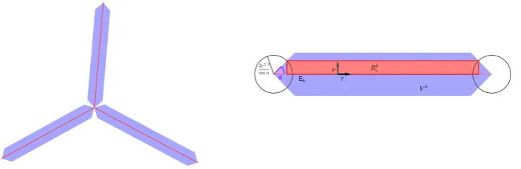
Figure 1.1: Typical shape of the sets Vk (left) and general construction involved in the

definition ofRk_ε (right).

Proof. Fix ϕ ∈C_c∞(Ωδ;RN−1) with ϕi ≥ 0 for any i= 1, . . . , N −1 and Ψ∗(ϕ(x)) ≤1

for all x∈Ωδ. By Remark 1.3.5 we have

c0

N−1 X

i=1 Z

Ωδ

ϕid|Du⊥i −Γi| ≤ N−1

X

i=1

lim inf

ε→0 Z

Ωδ

ϕieiε(uε,i)dx≤lim inf ε→0

N−1 X

i=1 Z

Ωδ

ϕieiε(uε,i)dx

≤lim inf

ε→0 F Ψ

ε (Uε,Ωδ),

and taking the supremum overϕwe get (1.3.9).

We now state and prove a version of an upper-bound inequality for the functionals FΨ

ε which will enable us to deduce the convergence of minimizers ofFεΨ to minimizers of

FΨ(U,Ωδ) =c0|DU⊥−Γ|Ψ(Ωδ), forU ∈SBV(Ωδ;ZN−1).

Proposition 1.3.9 (Upper-bound inequality). Let Λ = τ ⊗g· H1 _L _{be a rank one}

tensor valued measure canonically representing an acyclic graph L∈ G(A), and let U = (u1, . . . , uN−1) ∈ SBV(Ωδ;ZN−1) such that Du⊥i = Γi −Λi for any i = 1, . . . , N −1.

Then there exists a sequence {Uε}ε⊂H such that Uε→U in [L1(Ωδ)]N−1 and

lim sup

ε→0

F_εΨ(Uε,Ωδ)≤c0|DU⊥−Γ|Ψ(Ωδ). (1.3.10)

Proof. Step 1. We consider first the case Λi = τi · H1 λi with λi a polyhedral curve

transverse to γi for any 1 ≤ i < N. Then the support of the measure Λ is an acyclic

polyhedral graph (oriented by τ and with normal ν = τ⊥) with edges E0, . . . , EM and

vertices{S0, . . . , S`}*(∪iγi)∩Ωδ such thatEk = [Sk1, Sk2] for suitable indicesk1, k2 ∈ {0, . . . , `}. Denote also gk = g|Ek ∈ R

N−1 _{and recall} _gk

(27)

finiteness there exist η >0 and α ∈(0, π/2) such that given any edge Ek of that graph

the sets

Vk ={x∈_R2,dist(x, Ek)<min{η,cos(α)·dist(x, Sk1),cos(α)·dist(x, Sk2)}}

are disjoint and their union forms an open neighbourhood of∪iλi\ {S0, . . . , S`}(choose,

for instance, α such that 2α is smaller than the minimum angle realized by two edges and then pick η satisfying 2ηtanα <minjH1(Ej)).

For 0 < ε δ, let B_εm = n

x∈_R2 _: _|_x₋_S

m|< 3ε 2/3

sinα

o

, Bε = ∪mBεm and define

Rk_ε ⊂Vk as

Rk_ε ={y+tν : y ∈Ek,min{dist(y, Sk1),dist(y, Sk2)}>3ε2/3cot(α),0< t≤3ε2/3}.

Let ϕ0 be the optimal profile for the 1-dimensional Modica–Mortola functional, which solves ϕ0₀ = pW(ϕ0) on R and satisfies limτ→−∞ϕ0(τ) = 0, limτ→∞ϕ0(τ) = 1 and ϕ0(0) = 1/2. Let us define τε=ε−1/3,r+ε =ϕ0(τε),rε−=ϕ0(−τε), and

˜ ϕε(τ) =

       

      

0 τ <−τε−r−ε

τ+τε+r−ε −τε−rε−≤τ ≤ −τε

ϕ0(τ) |τ| ≤τε

τ−τε+r+ε τε ≤τ ≤τε+ 1−r+ε

1 τ > τε+ 1−rε+

Observe that (1−r_ε+) and r_ε− are o(1) as ε → 0. For x = y +tν ∈ R_εk let us define ϕε(x) = ˜ϕε t_ε−τε−rε−

, so that, asε→0,

Z

Rk ε∩Ωδ

ε|Dϕε|2+

1

εW(ϕε)dx≤ H 1₍_E

k∩Ωδ)

Z 2τε−rε−

−τε−rε−

|Dϕ˜ε(τ)|2+W( ˜ϕε(τ))dτ+o(1)

≤ H1(Ek∩Ωδ)

Z τε

−τε

2ϕ0₀(τ)pW(ϕ0(τ))dτ+o(1)≤c0H1(Ek∩Ωδ) +o(1).

Define, forx∈Ωδ\Bε,

uε,i(x) =

(

ui(x) +ϕε(x)−1 ifx∈(Rkε \Bε)∩Ωδ whenever Ek⊂λi

ui(x) elsewhere on Ωδ\Bε

and on Bε ∩Ωδ define uε,i to be a Lipschitz extension of uε,i|∂(Bε∩Ωδ) with the same

Lipschitz constant, which is of order 1/ε. Remark thatuε,i has the same prescribed jump

asui acrossγi, and thus FεΨ(Uε,Ωδ)<∞. Moreover,uε,i→ui inL1(Ωδ).

Observe now that ifEk is contained in λi∩λj then by construction

ei_ε(uε,i) =ejε(uε,j) =ε|Dϕε|2+

(28)

on ˜Rk_ε = (Rk_ε∩Ωδ)\Bε. Letϕ= (ϕ1, . . . , ϕN−1), withϕi ≥0 and Ψ∗(ϕ)≤1, we deduce

Z

Ωδ

X

i

ϕieiε(uε,i)dx≤ ` X k=1 Z ˜ Rk ε X i

ϕieiε(uε,i)dx+

Z

Bε∩Ωδ

X

i

ϕieiε(uε,i)dx

≤ ` X k=1 Z ˜ Rk ε X i

ϕigki

ε|Dϕε|2+

1 εW(ϕε)

dx+

Z

Bε∩Ωδ

Ψ(~eε(Uε))dx

≤ ` X k=1 Z ˜ Rk ε

Ψ(gk)

ε|Dϕε|2+

1 εW(ϕε)

dx+Cε1/3

≤

`

X

k=1

Ψ(gk)(c0H1(Ek∩Ωδ) +o(1)) +Cε1/3 ≤c0|DU⊥−Γ|Ψ(Ωδ) +o(1)

asε→0. In view of (1.3.8) we have

F_εΨ(Uε,Ωδ)≤c0|DU⊥−Γ|Ψ(Ωδ) +o(1),

and conclusion (1.3.10) follows.

Step 2. Let us now consider the case ΛL≡Λ =τ⊗g· H1 L,L=∪iλi and theλiare

not necessarily polyhedral. LetU ∈SBV(Ωδ;ZN−1) such that DU⊥= Γ−ΛL. We rely

on Lemma 1.3.10 below to secure a sequence of acyclic polyhedral graphsLn=∪iλni,λni

transverse to γi, and s.t. the Hausdorff distance dH(λni, λi)< 1_n for all i= 1, . . . , N−1,

and|Λ_L_n|_Ψ(Ωδ)≤ |ΛL|Ψ(Ωδ)+1_n. LetUn∈SBV(Ωδ;ZN−1) such that (DUn)⊥= Γ−ΛLn.

In particular, Un → U in [L1(Ωδ)]N−1 and by step 1 we may construct a sequence Uεn

s.t. U_εn→Un in [L1(Ωδ)]N−1 and

lim sup

ε→0

F_εΨ(U_εn,Ωδ)≤c0|(DUn)⊥−Γ|Ψ(Ωδ) =c0|ΛLn|Ψ(Ωδ)

≤c0|ΛL|Ψ(Ωδ) +

c0

n =c0|DU

⊥₋_Γ|

Ψ(Ωδ) +

c0 n.

We deduce

lim sup

n→∞ F

Ψ

εn(U

n

εn,Ωδ)≤c0|DU

⊥₋_Γ|

Ψ(Ωδ)

for a subsequenceεn→0 asn→+∞. Conclusion (1.3.10) follows.

Lemma 1.3.10. Let L∈ G(A), L=∪_iN₌₁−1λi, be an acyclic graph connectingP1, . . . , PN.

Then for any η > 0 there exists L0 ∈ G(A), L0 = ∪N_i₌₁−1λ0_i, with λ0_i a simple polyhedral curve of finite length connecting Pi to PN and transverse to γi, such that the Hausdorff

distance dH(λi, λ0i) < η and |ΛL0|_Ψ(_R2) ≤ |Λ_L|_Ψ(_R2) + η, where Λ_L and Λ_L0 are the

canonical tensor valued representations of L and L0. Proof. Since L ∈ G(A), we can write L = ∪M

m=1ζm, with ζm simple Lipschitz curves

(29)

Let ΛL=τ ⊗g· H1 L be the rank one tensor valued measure canonically representing

L, and let dm = Ψ(g(x)) for x ∈ ζm. The dm are constants because by construction

g is constant over each ζm. Now consider a polyhedral approximation ˜ζm of ζm having

its same endpoints, with dH( ˜ζm, ζm) ≤ η, H1( ˜ζm) ≤ H1(ζm) +η/(CM) (C to be fixed

later) and, for mi 6=mj, ˜ζmi∩ζ˜mj is either empty or reduces to one common endpoint.

Observe that whenever ζm intersects some γi, such a ˜ζm can be constructed in order

to intersect γi transversally in a finite number of points. Define L0 = ∪Mm=1ζ˜m and let

ΛL0 = τ0 ⊗g0 · H L0 be its canonical tensor valued measure representation. Then, by construction Ψ(g0(x)) =dm for any x∈ζ˜m, hence

|Λ_L0|_Ψ(_R2) =

M

X

m=1

dmH1( ˜ζm)≤ M

X

m=1 dm

H1₍_ζ

m) +

η CM

≤ |Λ_L|_Ψ(R2) +η,

providedC= max{Ψ(g) : g∈_RN−1_{, g}

i ∈ {0,1}for all i= 1, . . . , N−1}. Finally, remark

thatdH(L, L0)< ηby construction.

Thanks to the previous propositions we are now able to prove the following

Proposition 1.3.11 (Convergence of minimizers). Let {Uε}ε ⊂ H be a sequence of

minimizers for F_εΨ in H. Then (up to a subsequence) Uε→U in [L1(Ωδ)]N−1, and U ∈

SBV(Ωδ;ZN−1) is a minimizer of FΨ(U,Ωδ) =c0|DU⊥−Γ|Ψ(Ωδ) in SBV(Ωδ;ZN−1).

Proof. LetV ∈SBV(Ωδ;ZN−1) such thatDV⊥= Γ−Λ, where Λ canonically represents

an acyclic graphL∈ G(A), and letVε∈Hsuch that lim supε→0FεΨ(Vε,Ωδ)≤FΨ(V,Ωδ).

Since F_εΨ(Uε,Ωδ) ≤ FεΨ(Vε,Ωδ), by Proposition 1.3.7 there exists U ∈ SBV(Ωδ;ZN−1)

s.t. Uε →U in [L1(Ωδ)]N−1 and by Proposition 1.3.8 we have

FΨ(U,Ωδ)≤lim inf ε→0 F

Ψ

ε (Uε,Ωδ)≤lim sup ε→0

F_εΨ(Vε,Ωδ)≤FΨ(V,Ωδ).

Given a general V ∈ SBV(Ωδ;ZN−1) we can proceed like in Remark 1.2.9 and find V0

such thatDV0⊥= Γ−ΛL0 withL0 acyclic, andFΨ(V0,Ω_δ)≤FΨ(V,Ω_δ). The conclusion follows.

Let us focus on the case Ψ = Ψα, where Ψα(g) =|g|1/α for 0 < α≤1 and Ψ0(g) = |g|∞, and denote Fε0 ≡FεΨ0 and Fεα≡FεΨα. ForU = (u1, . . . , uN−1)∈H we have

F_ε0(U,Ωδ) =

Z

Ωδ

sup

i

ei_ε(ui)dx, Fεα(U,Ωδ) =

Z

Ωδ

N−1 X

i=1

ei_ε(ui)1/α

!α

dx, (1.3.11)

and

F0(U,Ωδ) :=c0|DU⊥−Γ|Ψ0(Ωδ) and F α₍_U,_Ω

δ) :=c0|DU⊥−Γ|Ψα(Ωδ), (1.3.12)

(30)

Theorem 1.3.12. Let {P1, . . . , PN} ⊂R2 such that maxi|Pi|= 1, 0< δ maxij|Pi−

Pj|, Ω =B10(0) and Ωδ= Ω\(∪iBδ(Pi)). For 0≤α≤1 and 0< εδ, denote Fεα,δ ≡

F_εα(·,Ωδ)andFα,δ ≡Fα(·,Ωδ), withFεα(·,Ωδ)(resp., Fα(·,Ωδ)) defined in (1.3.11)(resp.

(1.3.12)).

(i) Let {Uεα,δ}ε be a sequence of minimizers for Fεα,δ onH, with H defined in (1.3.5).

Then, up to subsequences, Uεα,δ → Uα,δ in [L1(Ωδ)]N−1 as ε → 0, with Uα,δ ∈

SBV(Ωδ;ZN−1)a minimizer ofFα,δ onSBV(Ωδ;ZN−1). Furthermore,Fεα,δ(Uεα,δ)→

Fα,δ(Uα,δ).

(ii) Let{Uα,δ}_δ be a sequence of minimizers for Fα,δ onSBV(Ωδ;ZN−1). Up to

subse-quences we haveUα,δ →Uα|Ωη in[L

1_(Ω

η)]N−1asδ→0for every fixedηsufficiently

small, with Uα ∈ SBV(Ω;ZN−1) a minimizer of Fα on SBV(Ω;ZN−1), and Fα

defined in (1.2.5), (1.2.6). Furthermore, Fα,δ(Uα,δ)→Fα(Uα).

Proof. In view of Proposition 1.3.11 it remains to prove item (ii). The sequence{Uα,δ_} δ

is equibounded inBV(Ωη) uniformly in η, hence Uα,δ → U in [L1(Ωη)]N−1 for allη >0

sufficiently small, with Uα ∈ SBV(Ω;ZN−1) and Fα,η(Uα) ≤ lim infδ→0Fα,η(Uα,δ) by lower semicontinuity of Fα,η. On the other hand, let ¯Uα be a minimizer of Fα on SBV(Ω;ZN−1). We have Fα,η(Uα,δ) ≤ Fα,δ(Uα,δ) for any δ < η, and by minimality,

Fα,δ(Uα,δ)≤Fα,δ( ¯Uα)≤Fα( ¯Uα)≤Fα(Uα). This proves (ii).

1.4

Convex relaxation

In this section we propose convex positively 1-homogeneous relaxations of the irrigation-type functionalsFα _{for 0}_≤_{α <}_{1 so as to include the Steiner tree problem corresponding}

toα= 0 (notice that the case α = 1 corresponds to the well-known Monge-Kantorovich optimal transportation problem with respect to the Monge cost c(x, y) =|x−y|).

More precisely, we consider relaxations of the functional defined by

Fα_{(Λ) =}_kΛk

Ψα =

Z

Rd

|g|₁_/αdH1 _L

if Λ is the canonical representation of an acyclic graphLwith terminal points{P1, . . . , PN} ⊂

Rd, so that in particular, according to Definition 1.2.1, we can write Λ = τ ⊗g· H1 L

with|τ|= 1,gi ∈ {0,1}. For any other d×(N −1)-matrix valued measure Λ on Rd we

setFα_{(Λ) = +∞.}

As a preliminary remark observe that, since we are looking for positively 1-homogeneous extensions, any candidate extensionRα _satisfies

Rα(cΛ) =|c|Fα(Λ)

for anyc∈_Rand Λ of the formτ ⊗g· H1 _L_{as above. As a consequence we have that} Rα_{(−Λ) =}_Rα_{(Λ), where}_{−Λ represents the same graph} _L _{as Λ but only with reversed}

(31)

1.4.1 Extension to rank one tensor measures

First of all let us discuss the possible positively 1-homogeneous convex relaxations ofFα

on the class of rank one tensor valued Radon measures Λ = τ ⊗g· |Λ|1, where |τ|= 1, g∈RN−1(cf. Section 1.2.1). For a generic rank one tensor valued measure Λ =τ⊗g·|Λ|1 we can consider extensions of the form

Rα(Λ) = Z

Rd

Ψα(g)d|Λ|1

for a convex positively 1-homogeneous Ψα on RN−1 (i.e., a norm) verifying

Ψα(g) =|g|₁_/α if gi∈ {0,1}for all i= 1, . . . , N−1,

Ψα(g)≥ |g|₁_/α for all g∈_RN−1. (1.4.1) One possible choice is represented by Ψα(g) = |g|₁_/α for all g ∈ _RN−1_{, while sharper} relaxations are given by, forα >0,

Ψα∗(g) =



 X

1≤i≤N−1

|g_i+|1/α 



α

+ 

 X

1≤i≤N−1

|g−_i |1/α 



α

, (1.4.2)

and for α= 0 by

Ψ0∗(g) = sup

1≤i≤N−1

g_i+ − inf 1≤i≤N−1g

−

i , (1.4.3)

with g_i+ = max{gi,0} and gi− = min{gi,0}. In particular, Ψα∗ represents the maximal

choice within the class of extensions Ψα satisfying

Ψα(g) =|g|₁_/α ifgi ≥0 for all i= 1, . . . , N−1.

Indeed, for α >0,g∈_RN−1 _and _g±_{= (}_g±

1, . . . , g

±

N−1), we have Ψα(g)≤Ψα(g++g−) = 2Ψα

1 2g

+₊1 2g

−

≤2

1 2Ψ

α₍_g+_{) +} 1 2Ψ

α₍_g−₎

= Ψα(g+) + Ψα(g−) =|g+|₁_/α+|g−|₁_/α= Ψα_∗(g).

The interest in optimal extensions Ψα on rank one tensor valued measures relies in the so-called calibration method as a minimality criterion for Ψα-mass functionals, as it is done, in particular, in [70] for (STP) using the (optimal) norm Ψ0∗.

(32)

Example 1.4.1. Consider the Steiner tree problem for {P1, P2, P3} ⊂R2. We claim that

a minimizer ofR0_{(Λ) =}R

R2|g|∞d|Λ|1 within the class of rank one tensor valued Radon

measures Λ = τ ⊗g· |Λ|₁ satisfying (1.2.2) is supported on the triangle L = [P1, P2]∪ [P2, P3]∪[P1, P3], hence its support is not acyclic and such a minimizer is not related to any optimal Steiner tree. Denoting τ the global orientation of L (i.e., fromP1 toP2,P1 toP3 and P2 toP3) we actually have as minimizer

Λ =τ ⊗

1 2,−

1 2

· H1 _[_P

1, P2] + 1 2, 1 2

· H1 _[_P

3, P2] + 1 2, 1 2

· H1 _[_P 3, P1]

.

(1.4.4) The proof of the claim follows from Remark 1.4.2 and Lemma 1.4.3.

Remark 1.4.2 (Calibrations). A way to prove the minimality of Λ =τ⊗g· H1 _L_within the class of rank one tensor valued Radon measures satisfying (1.2.2) is to exhibit a

calibration for Λ, i.e., a matrix valued differential form ω = (ω1, . . . , ωN−1), with ωj =

Pd

i=1ωijdxi for measurable coefficientsωij, such that

• dωj = 0 for allj= 1, . . . , N−1;

• kωk∗ ≤1, wherek · k∗ is the dual norm to kτ ⊗gk=|τ| · |g|∞, defined as

kωk∗ = sup{τtω g : |τ|= 1, |g|∞≤1};

• hω,Λi=P

i,jτiωijgj =|g|∞ pointwise, so that

Z

R2

hω,Λi=R0(Λ).

In this way for any competitor Σ =τ0⊗g0· |Σ|1 we havehω,Σi ≤ |g0|∞, and, moreover,

Σ−Λ =DU⊥, forU ∈BV(R2;RN−1), hence

Z

R2

hω,Λ−Σi= Z

R2

hω, DU⊥i= Z

R2

hdω, Ui= 0.

It follows

R0(Σ)≥ Z

R2

hω,Σi= Z

R2

hω,Λi=R0(Λ),

i.e. Λ is a minimizer within the given class of competitors.

Let us construct a calibration ω = (ω1, ω2) for Λ in the general case P1 ≡ (x1,0), P2 ≡(x2,0) and P3≡(0, x3), withx1<0,x1 < x2 and x3 >0.

Lemma 1.4.3. LetP1,P2,P3defined as above andΛas in(1.4.4). Considerω = (ω1, ω2)

defined as

ω1 = 1

2a[(x1+a)dx+x3dy], ω2= 1

2a[(x1−a)dx+x3dy], for (x, y)∈BL ω1 =

1

2b[(x2+b)dx+x3dy], ω2= 1

(33)

with BL the left half-plane w.r.t. the line containing the bisector of vertex P3, BR the

corresponding right half-plane and a = px2

1+x23, b = p

x2

2+x23. The matrix valued

differential form ω is a calibration for Λ.

Proof. For simplicity we consider here the particular case x1 =−1₂,x2= 1₂ and x3 =

√

3 2 (the general case is similar). For this choice ofx1,x2,x3 we have

ω1 = 1 4dx+

√ 3

4 dy, ω2=− 3 4dx+

√ 3

4 dy, for (x, y)∈R

2_{, x <}₀_,

ω1 = 3 4dx+

√ 3

4 dy, ω2=− 1 4dx+

√ 3

4 dy, for (x, y)∈R

2_{, x >}₀_.

The piecewise constant 1-formsωifori= 1,2 are globally closed inR2(on the line{x= 0}

they have continuous tangential component), kωk∗ ≤ 1 (cf. Remark 1.4.2), and taking

their scalar product with, respectively, (1,0)⊗(1/2,−1/2), (−1/2,√3/2)⊗(1/2,1/2) for x <0 and (1/2,√3/2)⊗(1/2,1/2) forx >0 we obtain in all cases 1/2, i.e.,|g|∞, so that

Z

R2

hω,Λi=R0(Λ).

Hence ω is a calibration for Λ.

Remark 1.4.4. A calibration always exists for minimizers in the class of rank one tensor valued measures as a consequence of Hahn-Banach theorem (see, e.g., [70]), while it may be not the case in general for graphs with integer or real weights. The classical minimal configuration for (STP) with 3 endpointsP1,P2andP3 admits a calibration with respect to the norm Ψ0_∗ inRN−1 (see [70]) and hence it is a minimizer for the relaxed functional

R0_{(Λ) =} _||Λ|| Ψ0

∗ among all real weighted graphs (and all rank one tensor valued Radon measures satisfying (1.2.2)). It is an open problem to show whether or not a minimizer of the relaxed functional R0_{(Λ) =}_||Λ||

Ψ0

∗ has integer weights.

1.4.2 Extension to general matrix valued measures

Let us turn next to the convex relaxation of Fα _{for generic} _d_×₍_N₋_{1) matrix valued}

measures Λ = (Λ1, . . . ,ΛN−1), where Λi, for 1 ≤ i ≤ N −1, are the vector measures

corresponding to the columns of Λ. As a first step observe that, due to the positively 1-homogeneous request on Rα_{, whenever Λ =}_p_{· H}1 _L₌_τ _⊗_g_{· H}1 _L_{, with}_|_τ_|₌_cte. and gi∈ {0,1}, we must have

Rα(Λ) = Z

Rd

|τ||g|₁_/αdH1 L= Z

Rd

Φα(p)dH1 L,

with Φα(p) =|τ||g|1/α defined only for matricesp∈K0 (+∞ otherwise), where

(34)

Following [43], we look for Φ∗∗_α, the positively 1-homogeneous convex envelope on

Rd×(N−1) of Φα. Setting q = (q1, . . . , qN−1), with qi ∈Rd its columns, we have that the

convex conjugate function Φ∗_α(q) = sup{q·p−Φα(p), p∈K0} is given by Φ∗_α(q) = sup

(

τt·q·g− |τ| · |g|₁_/α, |τ|=cte., g=X

i∈J

ei, J ⊂ {1, . . . , N−1}

) = sup    c 

τt· 

 X

j∈J

qj



− |J|α 

 , c≥0,|τ|= 1, J ⊂ {1, . . . , N−1}  

 .

Hence Φ∗_α is the indicator function of the convex set

Kα =  



q ∈_Rd×(N−1)_, X

j∈J

qj

≤ |J|α _∀_J _{⊂ {1}_{, . . . , N}₋_1}

 

 ,

and, in particular, forα = 0, it holds (cf. [43]) that

K0 =  



q∈Rd×(N−1),

X

j∈J

qj

≤1 ∀J ⊂ {1, . . . , N−1}  

 .

It follows that Φ∗∗_α is the support function ofKα, i.e., forp∈_Rd×(N−1)_,

Φ∗∗_α(p) = sup

q∈Kα

p·q= sup  

 p·q ,

X

j∈J

qj

≤ |J|α_{, J} _{⊂ {1}_{, . . . , N}₋_1}

 



. (1.4.5)

We are then led to consider, for matrix valued test functions ϕ = (ϕ1, . . . , ϕN−1), the relaxed functional

Rα(Λ) = Z

Rd

Φ∗∗_α (Λ) = sup ( _N₋₁

X

i=1 Z

Rd

ϕidΛi, ϕ∈Cc∞(Rd;Kα)

) .

Observe that for Λ a rank one tensor valued measure and α = 0 the above expression coincides with the one obtained in the previous section choosing Ψ0 _{= Ψ}0

∗.

In the planar case d = 2, consider a 2 ×(N − 1)-matrix valued measure Λ = (Λ1, . . . ,ΛN−1) such that div Λi = δPi −δPN. Fix a measure Γ as, for instance, in

Remark 1.2.6. We have div(Λ−Γ) = 0 in R2 and by Poincar´e’s lemma there exists

U ∈BV(R2;RN−1) such that Λ = Γ−DU⊥. So the relaxed functional reads

Eα(U) =Rα(Λ) for Λ = Γ−DU⊥, U ∈BV(R2;RN−1). (1.4.6)