This mine is mine!
How minerals fuel conflicts in Africa
∗Nicolas Berman† MathieuCouttenier‡ Dominic Rohner§ Mathias Thoenig¶
First version: July 2014 This version: August 4, 2016
Abstract. We combine geo-referenced data on mining extraction of 14 minerals with information on conflict events at spatial resolution of 0.5o×0.5ofor all Africa over 1997-2010. Exploiting exogenous variations in World prices, we find a positive impact of mining on conflict at the local level. Quan-titatively, our estimates suggest that the historical rise in mineral prices (commodity super-cycle) might explain up to one fourth of average violence across African countries over the period. We then document how the appropriation of a mining area by a fighting group contributes to the escalation from local to global violence. Finally, we analyze the impact of corporate practices and transparency initiatives in the mining industry.
JEL classification: C23, D74, Q34
Keywords: Minerals, Mines, Conflict, Fighting, Natural Resources, Rebellion
∗
We thank Gani Aldashev, Chris Blattman, Paola Conconi, Ruben Enikopolov, Nicola Gennaioli, Gianmarco Leon, Thierry Mayer, Hannes Mueller, Paolo Pinotti, Uwe Sunde, and Oliver Van den Eynde, five anonymous referees and seminar and conference audiences in Oxford (OxCarre), Aix-Marseille, Bern, Bonn, Ente Einaudi, Geneva, Graduate Institute, IPEG Pompeu Fabra, Lyon, Montpellier, Paris, Universitat Autonoma de Barcelona, Uppsala, Warwick, ABCA 2015 Berkeley, IEA World Congress Jordan, Workshop on “The Geography of Civil Conflict” in Munich, the Conference on the “Political Economy of Conflict and Development” in Villars, the “Workshop on Conflict” at Bocconi University, the “CAVE workshop” at Prio, and the workshop on the “Political Economy of Development and Conflict IV” in Barcelona for very useful discussions and comments. Special thanks to Elissaios Papyrakis for sharing with us his data on EITI membership. Andre Python, Quentin Gallea, Valentin Muller, Jingjing Xia and Nathan Zorzi provided excellent research assistance. Nicolas Berman thanks the A∗Midex for financial support (grant ANR-11-IDEX-0001-02 funded by the French government “Investissement d’Avenir” program). Mathieu Couttenier and Mathias Thoenig acknowledge financial support from the ERC Starting Grant GRIEVANCES-313327. Dominic Rohner acknowledges financial support from the ERC Starting Grant POLICIES FOR PEACE-677595. This paper features an online appendix (available on the authors’ websites) containing additional results and data description.
†
Aix-Marseille University (Aix-Marseille School of Economics), CNRS, EHESS, Graduate Institute Geneva and CEPR. E-mail: [email protected].
‡
University of Geneva (previously: University of Lausanne). E-mail: [email protected]
§
Department of Economics, University of Lausanne and CEPR. E-mail: [email protected].
¶
1
Introduction
Natural riches such as valuable minerals have often been accused of fueling armed fighting. A typical case that recently made the headlines is the heavy fighting that broke out between the Rizeigat and Bani Hussein, two Arab tribes, for the territorial control of the Jebel Amer gold mine in Darfur region, killing more than 800 people and displaced some 150,000 others since January 2013.1 Armed groups extract revenues from mines without necessarily directly managing them, and extorsion or bribing practices have been widely documented in mineral-abundant conflict areas. An example is the financial and logistical support provided by the mining company AngloGold Ashanti in 2003-2004 to the “Nationalist and Integrationist Front” (FNI), a rebel group operating in the gold-rich district of Ituri in Eastern DRC.2
The present paper investigates the impact of mining on conflict by using geolocalized data on conflict events and mining extraction of 14 minerals for all African countries over the 1997-2010 period. Our results show that mining activity increases conflicts at the local level and then spreads violence across territory and time by enhancing the financial capacities of fighting groups. Our empirical analysis is based on the combination of an original dataset,Raw Material Data (RMD), documenting the location and the types of mines and minerals, with theArmed Conflict Location Events Data (ACLED) that provides information on the location and type of conflict events and the involved actors. The units of analysis are cells of 0.5 × 0.5 degree latitude and longitude (approx. 55km×55km at the equator) covering all Africa. The use of geo-referenced information enables causal identification: Including country×year fixed-effects and cell fixed-effects, we exploit in most of our econometric specifications the within-mining area panel variations in violence due to changes in the World price of the main mineral extracted in the area.
In the first part of our analysis, we estimate the overall extent of mining-induced violence at the local level. We find a positive effect of mining activity on conflict probability: a spike of mineral prices increases conflict risk in cells producing these commodities. These results are robust to a variety of consistency checks. We also find that countries with less corrupt institu-tions and with lower religious fractionalization/polarization are less affected by mining-induced violence; however, we detect little effect of political institutions (e.g. democracy, rule of law, government effectiveness). Similarly we find that minerals associated with higher rents are par-ticularly conflict-prone. We then perform several quantification exercises to gauge the magnitude of the effect: A one-standard deviation increase in the price of minerals translates into an increase in probability of violence in mining areas from the benchmark 16.9% to a counterfactual 22.5%. When aggregated at the country level, the effect remains sizeable. Indeed we quantify the effect
1Fighters from the “Sudan Liberation Army” (SLA) have operated their own illicit gold mine in Hashaba to the
east of Jebel Amer to finance their fighting. Other prominent examples of rebels sustaining their fighting efforts with the cash from running mines include for example rebels groups operating in Sierra Leone and Liberia such as the “Revolutionary United Front” (RUF) that financed weaponry with “blood diamonds” (Campbell, 2002), or the case of Angola’s rebels from “Uni˜ao Nacional para a Independencia Total de Angola” (UNITA) that financed their armed struggle with diamond money (Dietrich, 2000). See Reuters, 8 October 2013, “Special Report: The Darfur conflict’s deadly gold rush”. Another typical example is the Marikana Mine Massacre, where in a wildcat strike at a platinum mine owned by Lonmin in the Marikana area, close to Rustenburg, South Africa in 2012 several dozens of people were shot. See BBC, 5 October 2012, “South African mine owner Amplats fires 12,000 workers”.
2Human Right Watch brief, 5 June 2005, “D.R. Congo: Gold Fuels Massive Human Rights Atrocities”. For the
of the historical rise in mineral prices between 1997 and 2010, which according to most scholars was mainly due to the sharp increase in the demand for minerals by emerging market countries such as China and India (Humphreys, 2010; Carter, Rausser and Smith, 2011). Our estimates suggest that the contribution of this so-called commodities super cycle to the average violence observed across African countries over the period lies between 14% and 24%.
In the second part of the paper we take a more global view and investigate the diffusion over space and time of mining-induced violence, a question of central importance for understanding how local conflicts escalate into regional or national wars. Looking at the nature of violent events, we find that mineral price spikes fuel both low-level violence (riots, protests) and organized violence (battles). The rationales behind each type of violence being different, we focus on battles involving African rebel groups over the period, and provide evidence that mines spread conflicts across space and time by making rebellions financially feasible. More precisely, we first show that spikes in the price of minerals extracted in the ethnic homeland of a rebel group tend to spatially diffuse its fighting operations outside its homeland. As a second and alternative strategy, we make use of the information contained in theacleddata on the winners and losers of particular battle events. We show that the appropriation of a mining area by a rebel group increases the probability that this group perpetrates violence elsewhere in the rest of the country in the following years. Quantitatively, our estimates suggest that every conquest of a mining area triples the subsequent fighting activity of a group.
Having documented how mining allows rebel groups to expand their fighting activities, we show in the last part of the paper that the characteristics and behavior of extracting companies are also key. Mining companies have indeed an ambivalent role: On the one hand, they may be willing to secure areas where they plan to operate; on the other hand, they may contribute to the diffusion of violence by financing/bribing rebel groups. We provide suggestive evidence in line with the second channel. Our results show that mining-induced violence is mainly associated with foreign ownership. Nevertheless, among foreign companies, the ones that operate in the least corrupt countries, and the ones that comply to Corporate Socially Responsible practices are asso-ciated with less violence. Finally, we evaluate the impact of the recent transparency/traceability initiatives that have been promoted by international agencies, and find some evidence that these top-down policies have been able to reduce the conflict risk.
Our paper contributes to the literature in several ways. First, we study resource abundance and conflict i) for all major minerals; ii) using data at a high spatial resolution; iii) covering all Africa and iv) going beyond pooled panel regressions. Second, we provide direct, large-scale evidence of how capturing a mining area affects the diffusion of conflict over space and time. This yields findings that are in line with the view that resource rents can fuel diffusion of fighting by making it feasible to sustain rebelion. Third, to the best of our knowledge we are the first ones to document how mining company characteristics and practices (e.g. size, location of headquarters, compliance to Corporate Social Responsibility) can contain or boost mining-induced violence.
companies and of transparency initiatives, and section 7 concludes.
2
Existing Evidence and Conceptual Framework
In the last ten years there has been an increasing interest of the empirical literature in linking natural resource abundance to civil conflict and other forms of violence.3 Most existing papers have estimate pooled cross-country regressions finding that civil war onset and incidence correlate positively with natural resources, generally focusing on oil, diamonds or narcotics.4 The main shortcoming of this “first generation” of papers is that resource-rich and resource-poor countries typically also differ in various geographic, demographic, political and economic dimensions, and the existence of unobserved heterogeneity makes it hard to give a causal interpretation to such cross-country correlations.
A more recent literature tries to take into account this issue through the use of panel data and the inclusion of country fixed-effects, focusing on variations in prices or resource discoveries as an identification device. This has led to contradictory results: While Lei and Michaels (2014) find a positive effect of oil discoveries on conflict, Cotet and Tsui (2013) find that oil discoveries do not have an effect on conflict anymore when controlling for country fixed-effects. Commodity price shocks also have an unclear effect on conflict, and are found in particular to be unrelated to conflict onsets (Bazzi and Blattman, 2014). One of the reasons for these contradictory results could be that having as unit of observation the country-year level is just too aggregate, as in many countries conflicts are concentrated in particular regions (think e.g. of the Niger delta in Nigeria or the Kurdish part of Turkey). Given this within-country heterogeneity, aggregating information into a country-year panel may lead to noisy estimates and hence attenuation bias. Recently, some papers have used disaggregated data on natural resources and conflict for one particular country, such as Dube and Vargas (2013) on oil in Colombia; Aragon and Rud (2013) on a gold mine in Peru; and Maystadt, de Luca, Sekeris and Ulimwengu (2014) on minerals in the DRC, as well as Sanchez de la Sierra (2015) on coltan and gold in Eastern Congo. However, there does not exist so far a study of the nexus between natural resources and conflict with a panel of disaggregated cells covering all minerals and a whole continent (Africa), as we use in the current paper. This yields a big gain in terms of external validity.
From a conceptual perspective, a rich theoretical literature has identified several major chan-nels through which natural resources magnify the risk of conflict –a survey relevant for our analysis being provided by Bazzi and Blattman (2014). First, natural resources improve rebellion feasabil-ity i.e. looting and extortion relax financing constraints and make it easier to set up and sustain a rebel movement. Second, the presence of natural resources increases the “prize” that can be seized through the capture of the territory or the state – which has been referred to as greed or
rent-seeking. Third,weak state capacity and extractive institutions may be a further consequence of resource wealth: Rentier states can rely on resource rents and do not build up enough state
3Natural resources have also been found to empirically matter for homicides (Couttenier, Grosjean and Sangnier,
2014), for organized crime (Buonanno, Durante, Prarolo and Vanin (2015), for interstate wars (Caselli, Morelli and Rohner, 2015) and for mass killings of civilians (Esteban, Morelli and Rohner, 2015).
4
capacity and good institutions, which makes them less effective in counterinsurgency and eventu-ally more instable. Fourth, given that natural resource production iscapital intensive, a resource price spike will boost capital-intensive production, and shrink labor-intensive sectors, which frees up cheap labor for rebellion. Fifth, natural resources can in addition exacerbategrievances, due to frustrations from environmental degradation or banned access to lucrative mining jobs. Sixth, mining booms could affect migration patterns and lead to changes in the size and composition of the local population in mining areas with respect to ethnicity, age and gender.5 Finally, there
is also a channel working in the opposite direction: Higher local incomes in mining areas may increase the opportunity cost of rebellion, which in turns decreases the likelihood of conflict.
The existing empirical literature has typically been unable to distinguish between these differ-ent theoretical mechanisms.6 In the first part of the paper, we document a positive causal impact of mineral prices variations on conflicts which is consistent with all those mechanisms (except the last one). However, in the second part of the paper we focus specifically on the feasability
channel. In particular, we find that territorial control of mining areas leads rebel groups to spread their fighting elsewhere in successive periods. We also find that foreign mining companies oper-ating in corrupt environments trigger more conflict, which is a piece of suggestive evidence of the participation of these companies in the financing of rebel groups. Overall, we see these results as supporting the existence of the feasibility channel. But this does in no way preclude that other mechanisms are jointly at work.
3
Data
3.1 Data description
The structure of the dataset is a full grid of Africa divided in sub-national units of 0.5×0.5 degrees latitude and longitude (which means around 55×55 kilometers at the equator). We use this level of aggregation rather than administrative boundaries to ensure that our unit of obser-vation is not endogenous to conflict events.7 Our unit of observation is therefore a cell-year in sections 4 and 6, i.e. we study how mineral resources affect the probability that a conflict takes place in a given cell, during a given year. In this section we provide information about the main datasets and variables used in the paper – more details appear in the online appendix, section A.
Conflict data. We use the Armed Conflict Location and Event dataset (Raleigh, Linke, and
Dowd, 2014) which contains information on the geo-location of conflict events in all African countries. We focus on the 1997-2010 period which overlaps with our mines data. We have information about the date (precise day most of the time), longitude and latitude of conflict
5
Forfeasability see Fearon (2004), Collier, Hoeffler and Rohner (2009), Nunn and Qian (2014), and Dube and Naidu (2015); for greed see Reuveny and Maxwell (2001), Grossman and Mendoza (2003), Hodler (2006), and Caselli and Coleman (2013); forstate capacity see Fearon (2005), Besley and Persson (2011) and Bell and Wolford (2015); forcapital intensive see Dal Bo and Dal Bo, (2011), Dube and Vargas, (2013); formigrationsee Le Billon (2001), Ross (2004), and Humphreys (2005).
6A notable exception is Humphreys (2005) who uses among others the distinction between production and
reserves to distinguish between different channels, estimating pooled cross-country regressions, as well as Morelli and Rohner (2015) and Dube and Vargas (2013) documenting the role of secession, and capital-intensiveness, respectively.
7
events within each country. These events are obtained from various sources, including press accounts from regional and local news, humanitarian agencies or research publications. A first unique feature of the acled dataset is that it records all political violence, including violence against civilians, rioting and protesting within and outside a civil conflict, without specifying a battle-related deaths threshold. Another is that it contains information on the type of events, their outcome, as well as the characteristics of the actors on both sides of the conflicts. We know in particular if the event was a battle, the names of the groups involved, and who won the battle.8
We shall make use of this information when testing for the channels of transmission.9
The latitude and longitude associated to each event define a geographical “location”. acled contains information on the precision of the geo-referencing of the events. The geo-precision is at least the municipality level in more than 95% of the cases, and is even finer (village) for more than 80% of the observations. We keep only events which are geolocalized with the finer precision level for our analysis, and we drop duplicated events.10
The data is aggregated by year and 0.5×0.5 degree cell. We construct a dummy variable which equals one if at least one conflict happened in the cell during the year, which we interpret as cell-specific conflict incidence. This is our main dependent variable throughout the paper. Alternatively, we compute a variable containing the number of events observed in the cell during the year, which we labelconflict intensity. We also show that our results are robust to modeling cell-specific conflict onset and ending separately.
While the geo-coding of the events is cross-checked in theacleddataset, it is not immune to potential biases and measurement errors. We cannot rule out the possibility that the reporting of conflicts is biased towards certain types of countries, regions or events, as some regions might in particular have better media coverage. An event dataset such asacledcannot, by definition, be fully exhaustive. Our empirical methodology makes it however unlikely that this affects our results, as structural differences in media coverage or more generally in the reporting of events is captured by cell and country-year fixed-effects.11
Mines data. To eachcell-year, we merge information on mines fromRaw Material Data(RMD,
IntierraRMG). The data contain information on the location of mines around the World since 1980.12 For each year, we know whether a mine is active or not, the year production started,
8Eight different types of events are included in
acled: battle with no changes in territory; battle with territory
gains for rebels; battle with territory gains for the government; establishment of a headquarter; non violent activity by rebels; rioting; violence against civilians; non violent acquisition of territory. Actors are classified according to the following typology: government or mutinous force; rebel force; political militia; ethnic militia; rioters; protesters; civilians; outside / external force (e.g. UN).
9The presence of this detailed information as well as the more exhaustive character of the
acledare the main
reason why we chose to use this dataset, rather than theucdp-geddataset. The latter records only deadly events pertaining to conflicts reaching at least 25 battle-related deaths per year, and does not include information on battle events outcomes. We nevertheless also show and discuss the results obtained using theucdp-geddataset in the online appendix (Section E).
10
This has no impact when considering conflict incidence, our main variable of interest, but reduces noise when looking at the number of events as we do in a robustness exercise.
11We also show that our results are obtained across events of different types (battles, riots, violence against
civilians). Similarly, when considering jointly acled and ucdp-gedevents, our coefficient of interest is similar for the two datasets, despite the fact that theucdp-geddataset is less exhaustive and records only large, deadly events which are arguably less likely to be affected by reporting bias.
12More information is available at http://www.snl.com/Sectors/metalsmining/Default.aspx. Other recent
the specific minerals produced and the total production for each of them. We use this data to identify active mining areas, and the type of minerals they produce. The dataset also includes additional information about the ownership structure and characteristics of the mines, as well as some data about extraction methods - we come back to these variables in Sections 4.5 and 6 in which we study the role of minerals’ and mining companies’ characteristics.
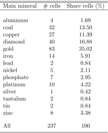
For each cell k, we defineMkt, a dummy variable which equals one if a least oneactive mine is recorded in the cell during year t. We identify 25 minerals in our sample of African countries. In the rest of the analysis we focus on the cells producing one or several of the 14 minerals for which we have price data.13 We define as the main mineral produced in the cell the mineral with the highest production over the entire period, evaluated at 1997 prices.14 Among the 237 mining cells for which a main mineral is identified, 70% produce a single mineral, and the main mineral produced represents on average 96% of total production value. In the robustness section, we show a number of robustness checks related to the definition of the main mineral; in particular we restrict our sample to single-mineral cells or consider all the minerals produced in a price index instead of the main mineral only.
Thermddataset collects information mostly for large-scale mines, usually operated by multi-nationals or the country’s government. Hence small-scale mines, and those that are illegally operated, are not included in our sample. While these measurement errors could lead to some attenuation bias in our estimates, we believe that this concern is limited in practice, given our empirical strategy. First, our baseline specifications include time-invariant versions of Mkt and identify the effect of mining through variations in World mineral prices within cells; in other words, measurement errors are unlikely to attenuate our estimates given the inclusion of cell fixed effects. Second, our unit of analysis being an area (i.e. a 0.5×0.5 degree cell) where mining takes place, we interpret our variable Mkt as a proxy for the extraction area of a given mineral rather than as coding for a specific rmd-referenced mine. If minerals are spatially clustered, these mining areas include all mines, including small ones. Note that we estimate a number of robustness tests to ensure that our results are not sensitive to changes in the definition of a mining area. In particular, we include the surrounding cells (first and second degrees) or use 1×1 degree units instead of 0.5×0.5. As shown later, results are consistent across specifications.
Other data. Information on the World price of the minerals is retrieved from the World Bank
Commodities prices dataset. Real prices are measured in constant 2005 USD. We also add dia-mond prices from Rapaport. Diadia-mond is problematic as its price varies importantly according to the quality and type of diamonds produced. There is a large heterogeneity in diamond qual-ity across mines and the price series for different qualities can move in opposite directions. As the rmd dataset contains no information on diamond quality, we exclude diamonds from our baseline sample in order to limit measurement errors. We however show that our results are
13
These minerals are: Bauxite (aluminum), Coal, Copper, Diamond, Gold, Iron, Lead, Nickel, Platinum (and Palladium/PGMs, i.e. Platinum Group Metals), Phosphate, Silver, Tantalum (Coltan), Tin and Zinc. These minerals are present in 92% of mining cells over our period of study. We do not consider the following minerals: Antimony, Chromite, Cobalt, Lithium, Manganese, Niobium, Rhodium, Tungsten, Uranium, Vanadium, Zirconium.
14
robust to the inclusion of this mineral. Similarly we add data on tantalum (coltan) price from the US Geological Survey. Unfortunately this series contains US unit values rather than a World price. To be consistent, we exclude tantalum from our baseline estimations and only keep the minerals for which World price data is available. Again, we show that adding coltan leaves our results largely unchanged. Finally, we add a number of cell-specific variables (distances, climate, ethnic homeland), country-specific data (institutions, social and ethnic cleavages, transparency initiatives) and mineral-specific information (extraction cost or method).
3.2 Descriptive statistics
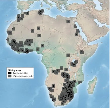
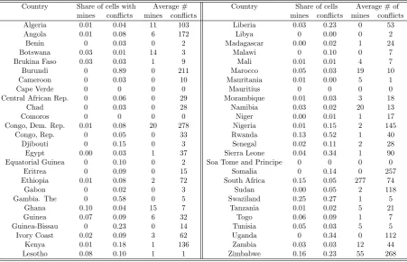
Our final sample covers 52 countries and 14 minerals –see Section A in the online appendix for a visual representation of the geo-localization of both conflict events and mines. Only four countries display no conflict events over the entire period and there are 20 countries with no active mine recorded. The main minerals present in the dataset are gold (a third of mining cells), diamond, copper and coal (around 10-15% each). Note that, except in the case of South Africa, the countries contained in our sample are typically small producers of the minerals from a World perspective: the average market share of a country-mineral is around 6.5% (the median at 2.9%), and drops to 4.5% when we exclude South Africa (and the median to 1.6%).
Table 1: Descriptive statistics: cell-level
Obs. Mean S.D. Median
Pr(Conflict>0)
all cells 144690 0.06 0.23 0
if mines>0 2798 0.14 0.35 0
if mines=0 141892 0.05 0.22 0
battles 144690 0.03 0.17 0
viol. against. civ. 144690 0.03 0.17 0
riots & protests 144690 0.02 0.12 0
# conflicts
all cells 144690 0.25 3.41 0
if>0 7980 4.61 13.79 2
Pr(Mine>0)
only cell 144594 0.02 0.14 0
incl. 1stsurrounding cells 144690 0.09 0.29 0
incl. 1st&2nd surrounding cells 144687 0.17 0.38 0
# mines
all cells 144594 0.05 0.60 0
if>0 2702 2.57 3.55 1
Pr(# mines>2)
all cells 144690 0.01 0.09 0
if mine>0 2798 0.40 0.49 0
Source: Authors’ computations from ACLED and RMD dataset.
neighboring cells (respectively, the first and second degree neighboring cells). Second, mines tend to be spatially clustered: conditional on observing at least one mine in a given cell, the average number of mines is 2.57. Finally, the conflict probability is much higher in cells with active mines, around 14%. Of course, this could be due to many unobserved cell characteristics, an issue we shall deal with in our estimations. In the online appendix (Section B) we document correlations between the presence of mining areas and the likelihood of violent events at the cell-level. We find that the presence of active mines is positively correlated with conflict incidence, both across and within cells.
4
Exogenous changes in the value of mines: Local impact
We turn now to our empirical analysis. First, our identification strategy is discussed and the baseline results are reported. Second, we provide a series of alternative specifications assessing the robustness of the results. Then we focus on heterogeneous effects. Finally, we perform various quantification exercises.
4.1 Methodological issues
Assessing the causal impact of mining on violence is subject to various methodological chal-lenges. The most obvious one relates to the reverse causation from local violence to mine open-ing/closing. The direction of this bias is most likely negative, i.e. conflict incidence might impact negatively the likelihood of a mine being active. This should therefore work against our finding of a significant positive correlation between mining activity and conflict. However, we cannot rule out the possibility that conflicts affect the value of a mine in a non-trivial way, for instance if the state uses part of the mine production to fight insurgency.15
In order to address causality, we focus on exogenous variations in the economic value of mines. The idea is that more valuable mines increase local rent-seeking and, consequently, the likelihood of violence.16 To abstract from local determinants of violence and guarantee exogeneity, we exploit the variations in the World prices of minerals. More precisely, we estimate a specification of the following form:
conflictkt=α1Mkt+α2lnpWkt +α3 Mkt×lnpWkt
+FEk+FEit+εkt (1)
where (k, t, i) denote respectively cell, time and country,FEk are cell fixed-effects andFEitis an additional battery of fixed-effects that can vary at different levels depending on the specification (e.g. year, country×year). Note that border cells are assigned to the country that represents the largest share of their area. The dependent variable,conflictkt, corresponds to the observation of violent events at the cell-year level where violence is measured in terms of incidence, i.e. a binary variable coding for non-zero events in theacleddataset on civil conflicts. Alternative measures of
15
Guidolin and La Ferrara (2007) actually find evidence that conflicts increase the value of extractive firms. They mention several reasons that might explain this finding: during conflict, (i) entry barriers might be higher; (ii) the bargaining power of governments might be lower and hence licensing cheaper; (iii) lower transparency leads to more unofficial deals which are profitable to the firms; (iv) the manufacturing sector leaves the country, forcing it to specialize in natural resources.
16
violence are considered in our sensitivity analysis in Section 4.3. The main explanatory variable, Mkt is a binary variable coding for the presence of at least one active mine at the cell-year level. The variable pWkt corresponds to the World price in year t of the main mineral produced by the mines present in cellk, i.e. the one with the highest total production (evaluated at 1997 prices) over the entire 1997-2010 period. For cells where no active mine ever produces over the period we set pWkt to zero; by contrast, it is non-zero for cells with a mine that is inactive only temporarily. Our sensitivity analysis investigates alternative coding rule forMkt andpWkt (Section 4.3).
In equation (1) we are primarily interested in the estimates of α3, the coefficient of the
interaction term between the price and the dummy for mining activity. This coefficient captures the impact on local violence of an exogenous increase in the World price of a given mineral, in cells where mining extraction of this mineral takes place. Given the fact that we include fixed-effects at the country-year level, our identification strategy relies on the exogeneity of the interaction term, Mkt×lnpWkt, with respect to the local determinants of conflict. We discuss hereafter this identification assumption.
Exogeneity of prices. This seems a reasonable assumption for the World price of minerals,
pWkt, as mentioned earlier. Still, one might argue that some mines are large enough to affect World prices, in which case the occurrence of conflict in these cells might also affect these prices. Although our sample contains only few countries with potentially large market power on the mineral market, we nevertheless test whether our results are robust to excluding from the sample all cells located in countries belonging to the top ten World producers of a specific mineral (see section H in the online appendix). Another possibility is that time-varying omitted variables could co-determine World prices and local violence in mining areas. The use of country×year fixed effects in our baseline specifications alleviates most of this problem, but we consider in our sensitivity analysis placebo exercises to ensure that our results are not driven by co-movements of the residual unobserved heterogeneity and the World prices of minerals.
Endogenous mining activity. As discussed above, potential reverse causation from conflicts
to mining opening/closing is an important concern. As a consequence, our coefficient of interest, α3, could be partly driven by conflict-induced shifts in the binary variableMkt. To account for this issue, we first restrict the estimate of equation (1) to the sub-sample of cells for which mining activity always takes place during the period (i.e. V(Mkt) = 0 for a givenk). Given thatMkt= 0 orMkt= 1 for all years, this variable is now absorbed by the cell fixed effects and the covariates lnpWkt and (Mk×lnpWkt) become identical; we accordingly include only the interaction term and the specification takes the following simpler expression:
conflictkt=α3 Mk×lnpWkt
+FEk+FEit+εkt (2)
This specification ensures that our coefficient of interest, α3, is identified within cells through
the changes in World commodity prices conditional on havingpermanently active mining activity (i.e. Mkt= 1 for all t), and not through the potentially endogenous opening/closing of mines.
An alternative way to get rid of endogenous mining activity consists in defining as mining areas cells where a mine has ever been recorded as active over the 1997-2010 period.17 Under
17
this coding rule the mining activity dummy becomes time-invariant, Mk ∈ {0,1}, such that the econometric specification is given by equation (2) and the coefficient of the interaction term α3
keeps on being identified through changes in World mineral prices only. The advantage of this approach is that it can be estimated on the full sample of cells and not on a selected sub-sample as is the case with the estimation based on cells without opening/closing of mines. Its disadvantage is that a cell can be considered a mining area even when mining does not necessarily take place in a given year.
Estimation issues. Due to the inclusion of several dimensions of fixed effects, we estimate
equations (1) and (2) using a Linear Probability Model in our baseline specifications. Non-linear estimators such as conditional logit or Poisson pseudo-maximum-likelihood estimator are implemented as robustness checks. Note also that with more than 900 country×year fixed effects in most specifications, estimating the large battery of fixed effects is very demanding from a data perspective. In this respect, keeping in the sample not only cells with mines but also the large number of cells with no mines (Mkt= 0 for all t) conveys information which is decisive for estimating these dummies. This is why we favor, in our baseline, specifications including the set of cells without mines, coding as zero the World price for these cells. Alternatively, we implement a neighbor-pair fixed effects methodology in the spirit of Acemoglu, Garcia-Jimeno and Robinson (2012) and Buonanno, Durante, Prarolo and Vanin (2015): Equation (2) is estimated on the sub-sample of mining cells and their immediate neighboring cells without mine. We define a neighborhood fixed effect that is specific to each (mine + neighbors) group. The price of the main mineral produced in the mining cell is also assigned to its neighbors. By contrast, the mining dummy can differ as it is set to zero in neighboring cells with no mine. Identification hence relies on relative variations in conflict incidence in the mining cell with respect to its neighboring cells when the World price of the main mineral changes. This approach is similar in spirit to a matching estimator. With a sample size reduction by a factor 10 this is a demanding specification. Its main benefit in our context is that it avoids coding to zero the log of mineral prices in cells with no mine.
Spatial correlation. Given the high spatial resolution of the data it is important to take into
account spatial correlation as both conflict and mines are clustered in space. Henceforth in all specifications standard errors are estimated with a spatial HAC correction allowing for both cross-sectional spatial correlation and location-specific serial correlation applying the method developed by Conley (1999) and Hsiang, Meng and Cane (2011). Our treatment is quite demanding as we impose no constraint on the temporal decay for the Newey-West/Bartlett kernel that weights serial correlation across time periods: The horizon at which serial correlation is assumed to vanish can be infinite (i.e. 100,000 years). In the spatial dimension we retain a radius of 500km for the spatial kernel– close to the median internal distance in our sample of African countries according to the CEPII geodist dataset.18
18
4.2 Baseline results
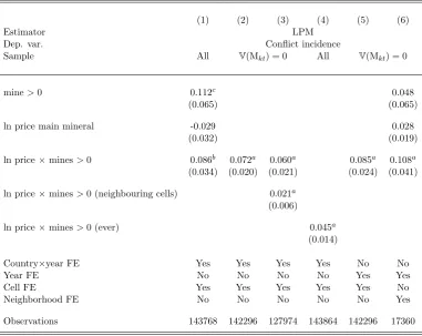
Table 2 reports the baseline results for various sample compositions and definitions of the variables. The dependent variable is conflict incidence. We see that in all columns, the interaction term between World price and local mining activity, our coefficient of interest, is positive and significant at the 1 or 5 percent level. Thus, a spike in mineral prices increases the conflict risk in cells producing these commodities. We estimate equation (1) on the full sample of cells. In column (1) mining activity (mine>0) is measured with a dummy taking the value 1 if at least 1 mine is active in the cell in yeart. Cell fixed effects are included with the purpose of controlling for time-invariant co-determinants of violence and mining at the local level – e.g. weak state capacity and property rights enforcement in remote places or latent political instability (e.g. ethnic cleavages). Country×year fixed effects are also included to filter out all countrywide time-varying characteristics affecting violence and activity of mines – e.g. a war-induced collapse of the central state and property rights.
Table 2: Conflicts and mineral prices
(1) (2) (3) (4) (5) (6)
Estimator LPM
Dep. var. Conflict incidence
Sample All V(Mkt) = 0 All V(Mkt) = 0
mine>0 0.112c 0.048
(0.065) (0.065)
ln price main mineral -0.029 0.028
(0.032) (0.019)
ln price×mines>0 0.086b 0.072a 0.060a 0.085a 0.108a (0.034) (0.020) (0.021) (0.024) (0.041)
ln price×mines>0 (neighbouring cells) 0.021a (0.006)
ln price×mines>0 (ever) 0.045a (0.014)
Country×year FE Yes Yes Yes Yes No No
Year FE No No No No Yes Yes
Cell FE Yes Yes Yes Yes Yes No
Neighborhood FE No No No No No Yes
Observations 143768 142296 127974 143864 142296 17360
LPM estimations. csignificant at 10%;bsignificant at 5%;asignificant at 1%. Conley (1999) standard errors in parentheses, allowing for spatial correlation within a 500km radius and for infinite serial correlation.mine>0 is a dummy taking the value 1 if at least 1 mine is active in the cell in yeart. mines>0 (ever) is a dummy taking the value 1 if at least 1 mine is recorded in the cell at any point over the 1997-2010 period. mines>0 (neighbouring cells) is a dummy taking the value 1 if at least 1 mine is recorded in neighbouring cells of degree 1 and 2 in yeart. V(Mkt) = 0 means that we consider only cells in which the mine dummy (or dummies in column (3)) takes always the same value over the period. Column (6) is estimated on a sample containing only mining cells and their immediate neighboring cells. In columns (1) to (5), ln price main mineral is the World price of the mineral with the highest production over the period (evaluated at 1997 prices) for mining cells, and zero for non-mining cells. In column (6) ln price main mineral takes the same value for the mining cell and its immediate neighbours. Estimations (1) and (6) include controls for the average level of mineral World price interacted with the mine dummy.
spatial lags of our explanatory variable by including the interaction term between mineral price and mining activity in neighboring cells of degrees 1 and 2.19 As shown by the coefficient of the second interaction term, we detect an impact on local conflict of mineral price shocks in neighboring cells. The effect is 60 percent lower than for the cell itself (i.e. the first interaction term) confirming that conflict tends to spill over with spatial decay, a feature that is likely to be driven by spatial diffusion of violence (e.g. rebels roaming around).20 In column (4) we use the alternative definition of mining activity where the mining dummy (mines>0ever) is now equal to one for cells where at least a mine has been recorded as active at any point over the 1997-2010 period. The coefficient of interest is slightly lower, an expected feature given that in this specifi-cation we define as mining areas places where mining took place in at least one year during the sample period. This leads to cells with currently inactive mines being treated as mining areas, resulting in potential attenuation bias.
The last two columns deal with alternative sets of fixed effects. Column (5) replicates column (2) without the country×year fixed effects. Indeed, with 15 percent of the cells belonging to more than one country, the interpretation of the unobserved heterogeneity that is captured by those fixed effects is unclear for border cells. We consequently use year fixed effects only. In the sensitivity analysis of the online appendix, section L we explore a more radical approach by dropping border cells. Column (6) implements the neighborhood fixed effects described earlier. We concentrate on the sample of mining cells and their immediate neighbours, and estimate the differential effect of mineral price variations in mining areas compared to their immediate neighbours. Our findings are confirmed: variations in mineral prices have a significantly higher effect in mining cells.
4.3 Sensitivity Analysis
In this subsection we show that the baseline estimates of Table 2 are robust to a large battery of sensitivity checks.
4.3.1 Mining activity
We start by investigating the robustness of our results to alternative definitions of mining activity, to further ensure that our results are not driven by endogenous opening/closing of mines (i.e. variations in the mining dummy over time). Tables are relegated to the appendix.
The first two columns of appendix Table 10 contain our two baseline ways of dealing with this potential reverse causation issue: considering only cells with permanently active mine (column (1), the same as column (2) in the Table 2), and using a time-invariant dummy for cells containing at least an active mine at any point over the 1997-2010 period (column (2), the same as column (4) in the Table 2). In column (3) of Table 10, we use a lagged mine dummy instead of the
19
More precisely, we also impose the constraint of no closing/opening mines for neighboring cells. Therefore ln price×mines>0 (neighboring cells) corresponds to the price of the main mineral produced among the neighboring cells with permanent mining activity.
20Our favorite interpretation of the results in column (3) is that violence diffuses in space. Henceforth this
contemporaneous value. The estimated coefficient remains positive but becomes slightly insignif-icant – but this is not our preferred way of dealing with reverse causality, as mining activity can be affected by anticipation of future conflicts. In column (4), the mining variable is coded as 1 from the first year onwards when an active mine is observed over the 1997-2010 period, 0 if no active mine was ever recorded, and is coded as missing otherwise. Finally, we use mining activity at beginning of the period (column (5)) or in the pre-sample period (5 years in column (6) and entire pre-sample period covered by the RMD data in column (7)). Our coefficient of interest is always highly significant and quantitatively stable.21
We also inquire robustness to alternative size of the mining area. As discussed in Section 3, the RMD dataset does not survey small-scale (potentially illegally operated) mines. Because of spatial clustering of mineral deposits, our main explanatory variable, Mkt, must be interpreted as a proxy for the extraction area of a given mineral rather than as coding for a specific RMD-referenced mine. But mining areas could on average be larger than our cells of a spatial resolution of 0.5×0.5 degree. Focusing on the impact of mines on the conflict likelihood in its surrounding cell of 0.5 ×0.5 degree may underestimate the real impact of being in a mining area. Hence, in Table 11 in the appendix we broaden the scope of a mining area and we reproduce Table 2 for a grid of cells at a larger resolution (1 degree ×1 degree).
4.3.2 Main mineral and mineral prices
Another important element of our analysis is the way in which we define the main mineral produced in the cell. Note that this has no impact on cells producing a single mineral – which represent 70% of mining cells. For the others, we use the price of the mineral with the highest production over the period, evaluated at 1997 prices. In Table 12 in the appendix we show that alternative coding choices deliver similar results. We consider our preferred baseline specifications, columns (2) and (4) of Table 2. We keep our baseline definition of the main mineral but restrict the sample, either to mining cells producing a single mineral over the entire period (columns (1)-(2)) or to cells for which the main mineral is the same for each year of the sample (columns (3)-(4)). In columns (5) and (6), we replace the price variable by the average price of all the minerals produced in the cells (for which we have a price), with weights equals to the share of each mineral in total production value over the period.
We also perform a series of consistency checks on mineral prices. In particular, we want to rule out that time-varying omitted variables could co-determine World prices and local violence in mining areas. Indeed, it could be the case that the residual unobserved heterogeneity still co-moves with the World prices of minerals despite the wide array of fixed effects we include. We perform a placebo analysis to exclude this last concern and check the validity of our approach. Our idea is to replace the price of the mineral produced in the cell by the price of a mineral that is not produced in the cell. More precisely, we randomly assign a mineral to each of the mining cells and estimate specifications (2) and (4) of Table 2 with this fakeMkt×lnpWkt variable. We repeat this Monte Carlo procedure in 1,000 draws. Figures 3.a and 3.b in the Appendix display the sampling distribution of the coefficient of the interaction term for each specification. Reassuringly, the Monte Carlo coefficients are distributed far from their baseline estimates and are
21An alternative way of considering this endogeneity issue is to instrument the mining dummy in the sample
massively insignificant. This confirms that our baseline results are not driven by co-movements in mineral prices.
4.3.3 Alternative definitions of violence
In all tables we focus on conflict incidence, which reflects our interest in explaining the general presence of conflict. In this section we test for robustness to alternative measures of conflict in terms of intensity, onset and ending. We first look at intensity of violence as measured by the yearly number of acled events reported in a given cell. The results are displayed in appendix Table 13 where columns (2) and (4) of the baseline Table 2 are replicated in panels A and B, respectively. For each panel, column (1) reports the LPM estimation results for the full sample. The distribution of the number of events being right-skewed due to over-reporting of intense events in acled22, we deal with outliers by winsorizing at top 5% in column (2) and at 2SD above the mean in column (3). We re-do the same exercises in columns (4)-(6) with a Poisson pseudo-maximum likelihood estimator – a well adapted procedure for count data. The results are again better estimated when extreme values are treated. This feature suggests that mineral prices impact violence intensity in a non-linear (concave) way. We investigate further this interpretation in the last two columns by estimating a LPM on the full sample with a log(1 +x) transformation of the LHS variable (column 7) and an inverse hyperbolic sine transformation (column 8). Finally we study cell-specific onsets and endings of conflict separately in the Section D of the online appendix, and in particular in Tables A.6 and A.7. Note that this exercise has a limited scope in the context of our spatial micro-data where, at the cell-level, the vast majority of events is short-lived.23 Finally, we complement our sensitivity analysis on violence measurement
by using an alternative conflict database with geo-coded information, namely the Conflict Data Program Geo-referenced Events Dataset (ucdp-ged). Theucdp-gedfocuses on deadly incidents associated with civil wars, as identified by the ucdp-prio Armed Conflict Database. All these results are displayed and discussed in the section E of the online appendix.
4.3.4 Other robustness checks
We perform various additional sensitivity checks that are discussed in details in the online appendix. For the sake of brevity we only list them here: (i) we investigate alternative spatial and temporal kernels in the computation of standard errors (section F); (ii) we instrument World prices × actual mines, using World prices × historical mines as instrument (section G); (iii) we remove from the estimation sample all cells located in a top-10 World producer of the main mineral produced in the cell (i.e. countries that could have some influence on World prices) (section H); (iv) we show that our results are robust to the inclusion of diamond and coltan (tantalum) mines in the sample and we also show that they are not driven by any specific mineral, by excluding sequentially each mineral from the sample (section I); (v) we use a non-linear (logit)
22
Take for example the following event: “CNDD rebels attacked Kazirabageni in Makamba Province. They clashed with security forces and 15 people were killed”. It takes place from the 17 to the 22 April 2002 and each day is coded as separate event inacled.
23Indeed the potential issue with using conflict incidence as a dependent variable has been raised by the
fixed-effects estimator instead of a LPM (section J); (vi) we use, instead of our binary mining variable, the number of mines or total production of the main mineral as measures of the intensity of mining activity in the cell (section K); (vii) border cells are removed from the sample to ease the interpretation of the country ×year fixed effects (section L); (viii) we consider price shocks in log-differences rather than in levels (section M); (ix) we include time-varying climate variables (rainfall and temperature) which might be correlated with commodity price variations (section N); (x) We test for non-classical measurement errors affecting our mining data points following the approach by Koenig, Rohner, Thoenig and Zilibotti (2015) (section O).
4.4 Country characteristics and mining induced violence
Is the abundance of valuable mines always a curse for political stability? Countries’ institu-tions and social characteristics may play a decisive role. In particular, minerals could exacerbate instability in countries where the conflict risk is already latently present due to social cleavages or weak institutions. This would be in line with the idea that minerals are not necessarily the deep cause of conflict but make them feasible – a mechanism we shall investigate in detail in the second part of the paper. In this sub-section we consider how country characteristics may modify the average effect of mineral price variations on local conflicts.
4.4.1 Domestic Institutions: Can Good Governance Stop the Guns?
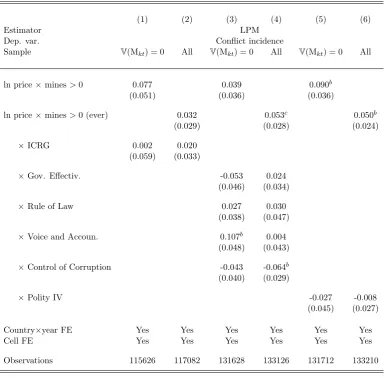
While natural resources have often been thought of as affecting the nature and quality of institutions (e.g., as generating corruption, autocracies and more generally a weaker accountability of the state), only relatively little attention has been paid to the impact of the interaction between institutional quality and natural resource abundance on political stability and prosperity.24 There are indeed reasons to expect natural resource extraction to have a stronger impact in weak states: it might for example be easier for local armed groups to extract rents from mining areas in such countries. Starting from our preferred specifications (columns (2) and (4) of Table 2) we now consider the triple interaction between our main explanatory variable (Mk×lnpWkt) and a country-level index of institutional qualityiqi— a binary variable equal to 1 when a country’s pre-sample (1996) institutional score is above the sample median.25
Table 3 displays the results. As our variable of interest varies across countries, we cluster stan-dard errors at this level. In columns (1)-(2), the variable iqi corresponds to the ICRGIndicator of Quality of Government from the International Country Risk Guide, a standard and synthetic measure of institutional quality at the country-level. In both specifications, the coefficient of the triple interaction is far from statistical significance. This measure being very coarse, in the follow-ing specifications (3)-(4) we draw on four more specific indicators of institutional quality, makfollow-ing use of the WGI (“Worldwide Governance Indicators”) dataset from Kaufmann, Kraay, and Mas-truzzi (2013).26 The coefficients of the triple interaction with Government Effectiveness
24
One of the most prominent empirical findings is by Mehlum, Moene and Torvik (2006) who show that natural resources hamper economic growth only in the presence of bad institutions. There is also a study by Andersen and Aslaken (2008) that distinguishes different types of democratic institutions in the context of a cross-sectional analysis with economic growth as dependent variable. Our exercise is quite different, as we use disaggregated data and consider conflicts, not economic growth, as a dependent variable.
25
We use pre-sample scores to mitigate endogeneity concerns. We focus on the year 1996 as many of the institutional variables are not available for earlier years.
26
Table 3: Heterogeneous effects: Institutional Quality
(1) (2) (3) (4) (5) (6)
Estimator LPM
Dep. var. Conflict incidence
Sample V(Mkt) = 0 All V(Mkt) = 0 All V(Mkt) = 0 All
ln price×mines>0 0.077 0.039 0.090b
(0.051) (0.036) (0.036)
ln price×mines>0 (ever) 0.032 0.053c 0.050b
(0.029) (0.028) (0.024)
×ICRG 0.002 0.020
(0.059) (0.033)
×Gov. Effectiv. -0.053 0.024
(0.046) (0.034)
×Rule of Law 0.027 0.030
(0.038) (0.047)
×Voice and Accoun. 0.107b 0.004 (0.048) (0.043)
×Control of Corruption -0.043 -0.064b (0.040) (0.029)
×Polity IV -0.027 -0.008
(0.045) (0.027)
Country×year FE Yes Yes Yes Yes Yes Yes
Cell FE Yes Yes Yes Yes Yes Yes
Observations 115626 117082 131628 133126 131712 133210
LPM estimations.csignificant at 10%;bsignificant at 5%;asignificant at 1%. Standard errors clustered by country in parentheses. mine>0 is a dummy taking the value 1 if at least 1 mine is active in the cell in yeart. mines>0 (ever) is a dummy taking the value 1 if at least 1 mine is recorded in the cell at any point over the 1997-2010 period. V(Mkt) = 0 means that we consider only cells in which the mine dummy takes always the same value over the period. ln price main mineral is the World price of the mineral with the highest production over the period (evaluated at 1997 prices) for mining cells, and zero for non-mining cells. Country-level variables are dummies taking the value 1 if the country is above the sample median of the corresponding variable before the start of the period.
and withRule of Law are not statistically significant. In contrast, the coefficient of the triple interaction with Voice and Accountability is in both columns of positive sign, and signif-icant in column (3) while not statistically signifsignif-icant in column (4). Taken at face value, this indicates that mining price shocks may have a stronger effect on civil conflict and unrest in places with greater voice and accountability. Further, the coefficient of the triple interaction with
Control of Corruption has in both columns a negative sign, and is statistically significant
in column (4), indicating that the impact of mining price spikes on conflict may be lower in
These four individual measures are mapped into clusters of key dimensions of government quality, with higher scores indicating better governance. Government Effectivenesscaptures “perceptions of the quality of public services, the quality of the civil service and the degree of its independence from political pressures, the quality of policy formulation and implementation, and the credibility of the government’s commitment to such policies”.
Rule of Law captures “perceptions of the extent to which agents have confidence in and abide by the rules of
countries putting in place better anti-corruption measures. Finally, in columns (5) and (6) we make use of the standard democracy score of Polity IV, which relates to governance and civil servant behavior, as well as political representation and free elections. The triple interaction has a negative sign but is not statistically significant.
In a nutshell, we do not detect strong heterogeneous effects for different institutional arrange-ments. Note that our country-level institutional measures are crude proxies, and our results may suffer from attenuation bias. Indeed, in the last section of the paper we show that anti-corruption and transparency measures have significant impact on specific types of events and mining companies.27
4.4.2 Inequality and Diversity: How Does the Social Fabric Matter?
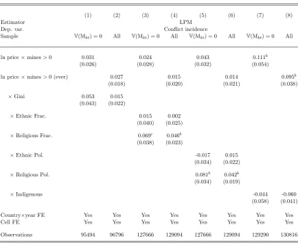
Social cleavages are considered in the literature as important sources of grievances and con-flicts. A natural question consists in assessing whether they also amplify mining-induced vio-lence.28 In the following we consider a battery of alternative indicators of social cleavages at the country-level, namely economic inequality, ethnic and religious fractionalization and polarization, as well as indigenous groups presence. We follow the same methodology as in Table 3 by esti-mating the coefficient of the triple interaction between our main explanatory variable and each of these indicators.
The results are reported in Table 4. In columns (1) and (2) we focus on the Gini index of gross income distribution of the “Standardized World Income Inequality Database” (Solt, 2014). Higher Gini scores correspond to larger inequality. The coefficient of the triple interaction is positive but not statistically significant. Columns (3) to (6) study the heterogeneous effect of ethnic and religious fractionalization or polarization (all variables are from Reynal-Querol, 2014) on price spikes. The coefficients of the triple interactions with religious fractionalization (columns (3) and (4)) or polarization (columns (5) and (6)) have a positive sign and are statistically significant. Note that this result survives to including fractionalization and polarization variables simultaneously. On the other hand, no significant effect is found for ethnic fractionalization or polarization. Finally, we assess the heterogeneous effect of indigenous group presence. We build the binary variable Indigenous that takes a value of 1 if all groups in a given cell are indigenous.29 The coefficient of the triple interaction with this variable has a negative sign but is not statistically significant at conventional levels. Taken together, the results of this subsection suggest that mineral price increases have the strongest conflict-inducing effects in religiously divided places.
27In Section P in the online appendix we study how a specific type of corruption – at the port – affects the impact
of mineral prices variations on conflict. We find evidence of a conflict inducing effect of our proxy of port-level corruption.
28
There is a small literature finding that the resource curse is mostly present in ethnically fractionalized countries. In particular, Hodler (2006) finds for a cross-section of 92 countries that natural resources reduce economic output only when ethnic or religious fractionalization is large.
29
Table 4: Heterogeneous effects: Cleavages
(1) (2) (3) (4) (5) (6) (7) (8)
Estimator LPM
Dep. var. Conflict incidence
Sample V(Mkt) = 0 All V(Mkt) = 0 All V(Mkt) = 0 All V(Mkt) = 0 All
ln price×mines>0 0.031 0.024 0.043 0.111b
(0.026) (0.028) (0.032) (0.054)
ln price×mines>0 (ever) 0.027 0.015 0.014 0.095b
(0.018) (0.020) (0.021) (0.038)
×Gini 0.053 0.015
(0.043) (0.022)
×Ethnic Frac. 0.015 0.002
(0.040) (0.025)
×Religious Frac. 0.069c 0.046b
(0.038) (0.023)
×Ethnic Pol. -0.017 0.015
(0.034) (0.022)
×Religious Pol. 0.081b 0.042b
(0.034) (0.019)
×Indigenous -0.044 -0.060
(0.058) (0.041)
Country×year FE Yes Yes Yes Yes Yes Yes Yes Yes
Cell FE Yes Yes Yes Yes Yes Yes Yes Yes
Observations 95494 96796 127666 129094 127666 129094 129290 130816
LPM estimations. csignificant at 10%;bsignificant at 5%;asignificant at 1%. Standard errors clustered by country in columns (1) to (6); Conley (1999) standard errors in parentheses, allowing for spatial correlation within a 500km radius and for infinite serial correlation in columns (7) and (8). mine>0 is a dummy taking the value 1 if at least 1 mine is active in the cell in yeart. mines>0 (ever) is a dummy taking the value 1 if at least 1 mine is recorded in the cell at any point over the 1997-2010 period.V(Mkt) = 0 means that we consider only cells in which the mine dummy takes always the same value over the period. ln price main mineral is the World price of the mineral with the highest production over the period (evaluated at 1997 prices) for mining cells, and zero for non-mining cells. In columns (1) to (6), country-level variables are dummies taking the value 1 if the country is above the sample median of the corresponding variable before the start of the period. In columns (7) and (8) the “Indigenous” variable is a dummy taking a value of 1 if all groups in a given cell are indigenous.
4.5 Mineral characteristics
We now study whether our results generalize to all types of minerals or if some sub-group of minerals with specific characteristics are particularly conflict-prone.
Labor-versus capital-intensiveness. The labor-versus capital-intensiveness of a given
methods and types of mines and opaque communication of commodity firms. Note also that our exercise has limited comparability with Dube and Vargas (2013) because variation in capital intensiveness between coffee and oil productions is huge while in our case, cross-mineral variations in capital intensiveness is modest.
We consider three different proxies of capital intensiveness using data from rmd. For a given metal, open cast is defined as the average percentage of mines in Africa that use -at least for part of their extraction- the open-cast, resp. open-pit mining method. Open-cast is often argued to be a particularly capital-intense mining method.30 The second proxy,energy intensity, cor-responds to the ratio of ln(Energy/Production) over ln(Employees/Production). The third proxy,
mine age, is the number of years since mining activity started in a given cell with the assumption
that older mines should on average be relatively less capital-intensive. Obviously mine age is a crude proxy of capital intensiveness and it may also correlate with other factors, such as e.g. en-vironmental grievances of local stakeholders. Results are shown in Table 14 in the appendix. We focus on the triple interaction term between our main explanatory variable (Mk×lnpWkt) and each proxy of capital intensiveness. None of these coefficients is statistically significant. A possible interpretation is that all our minerals are capital intensive in absolute terms, and that they are not different enough in terms of technology to have detectable heterogeneous effects on conflicts.31
Lootability and bulkiness. The literature has argued that more precious commodities
gener-ating larger rents are more conducive to fighting. Larger rents do not only increase the “prize” to be appropriated in contest by the winner, but also constitute attractive opportunities for loot-ing durloot-ing the conflict, helploot-ing rebel groups to fund their activities. Further, the recent paper by Sanchez de la Sierra (2015) makes the point that bulky commodities leads violent actors to impose monopolies of violence and sustain taxation.
We consider three different proxies of mineral lootability to study how proxies for minerals’ lootability/bulkiness may affect the nexus between price spikes and fighting (see Table 15 in the appendix and Section A in the online appendix for data information). First, we split the set of minerals into high vs low value-to-weight minerals. We interact our main explanatory variable with two mutually exclusive dummies coding for minerals with a 1997 price (in USD per ton) above or below the sample median. We find that the coefficient of interest is equal to 0.046 for minerals below median price, while for mineralsabove median price the analogous co-efficient is almost twice as large (column (1)). A similar picture emerges in column (2). This suggests that price spikes of more precious metals have a stronger conflict-inducing effect – con-sistent with recent evidence on mineral discoveries from Smits, Tessema, Sakamoto and Schodde (2016). Second, we interact the mining price shock with the variable rents that corresponds to the mineral-specific ratio of price over cost for all African mines. The coefficient of the triple
30Open-cast is often argued to be less labor intensive than underground mining: “Underground methods from
deep deposits (which) are generally more labor-intensive and expensive to mine than deposits mined by open-pit methods.”(ILO, 1990: 18).
31
interaction is non-significant (columns (3) and (4)). Last, we interact our price shock variable with a measure of average metal concentration in its corresponding ore. Bulky metals like e.g. platinum, are usually very diluted in the stone, which is why they are so expensive, while cheaper ones like iron have a larger ore grade.32 We find that the coefficient of the triple interaction is negative and significant (columns (5) and (6)), suggesting that bulky/diluted metals entail a larger conflict risk when prices spike. This could be driven by the fact that they are more valu-able, increasing the potential for looting. Moreover mining companies extracting bulky minerals have also a hard time to hide production, making it easier for armed groups to control the mining site and engage in extortion.
4.6 Quantification
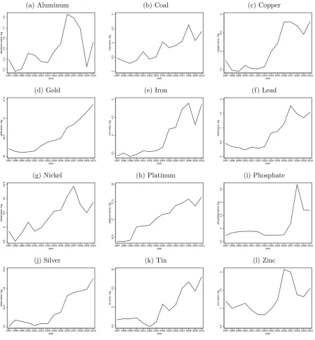
How large is the effect of mineral price variations on the conflict probability? Taking the baseline specification of Table 2, column (2), a one SD increase in the price of all minerals from their mean translates into an increase in probability of violence from 0.169 to 0.225. This is of sizeable magnitude, but concerns only the cells where active mining takes place. When we also consider the surrounding cells (Table 2, column (3)), conflict probability rises from 0.197 to 0.253. Over the period of our study mineral prices more than doubled on average.33 For instance, in constant 2005 USD, the ounce of gold was valued at $338 in 1997, and reached $1084 in 2010. This spectacular rise of mineral prices over the 2000-2009 period, known as the2000s commodity boom
or commodities super cycle has attracted quite a lot of attention. There is a consensus among scholars that no contraction of resource supply is to blame, but rather a rapid and substantial increase in demand, particularly so from the BRICS countries. As pointed out by Carter, Rausser and Smith (2011), “strong global demand, especially in lower-middle-income countries” helped set the stage for this commodity price boom, and “this strong demand was reflected in low real interest rates, a declining U.S. dollar, and strong GDP growth, and it contributed to the reduction in inventory levels that made commodity markets vulnerable to supply and demand shocks” (2011: 107). Similarly, Humphreys (2010) points out that the great metals boom between 2003 and 2008 “can be readily explained by the unusual strength of the demand shock and the lagged response of the supplying industry, with prices receiving an additional boost from the activities of commodity investors” (2010: 1).
What has been the effect of the commodity super cycle on conflicts in Africa? In Figure 1, we compute, for each country with recorded mines, the contribution to the observed violence of this historical rise in mineral prices (see Figures A.7 and A.8 in the online appendix for the map equivalent). The quantification being related to the number of conflict events, our exercise (left panel) is based on the PPML estimates from Table 13. Nevertheless we also include the quantification based on LPM estimates from Table 13 for the sake of robustness (right panel).34
32It is important to keep in mind that we focus here on large-scale industrial mining production. Some precious,
very diluted metals like gold may be “bulky” in industrial production yet much less bulky when extracted in artisan, alluvial depletion
33Prices have been multiplied by 2.8 in constant USD. Figure A.4 in the online appendix, section A shows the
evolution of the price of each of the minerals.
34More precisely, we compute the counterfactual share of events that would not have happened if prices had
Figure 1: The contribution of rising mineral prices to violence in Africa
(a) PPML (b) LPM
0 .2 .4 .6 .8 1
Share of events explained by increase in mineral prices
MRT BWAGHA MLI BFA LSO MARTUN ZAF NAMZMB TZAGIN TGO BENCIV EGY MOZSEN DZA NER ZWELBR CODSLE NGA SDN KEN RWAETH GNBBDI AGO
0 .2 .4 .6 .8 1
Share of events explained by increase in mineral prices
MRT BWAGHA MLI BFA LSO MARTUN ZAF NAMZMB TZAGIN TGOCIV EGY BEN SEN ZWEDZA MOZNER LBR CODSLE NGA SDN KEN RWAETH GNBBDI AGO
Note: These figures represent for each country the counterfactual share of events that would not have happened if prices had stayed stable at their 1997 level across the entire period. Predictions are based on an estimation similar to Table 13, Panel B, column (5) and (2) except that we also include the interaction term between mineral prices and the mining dummy for neighbouring cells.
In both cases the effect is highly heterogeneous across countries. Averaging across all countries with at least one recorded mine, we find that the historical rise in mineral prices contributed on average to 24% of the observed country-level violence using PPML estimates (14% using LPM). As is apparent in Figure 1, this number is however inflated by countries, such as Mauritania, in which only few conflict events are recorded (see online appendix Table A.3).35 Effects are on average larger when computations are based on the sample with permanently active mines (see Table A.9 in the online appendix).
We have several reasons to believe that these numbers are conservative estimates. First, our dataset is not exhaustive: only two percent of the cells contain active mines; we consider surrounding cells as well, but many small-scale mines are not included, although they may have a significant impact on violence, adding up to the one we identify here; further, not all minerals are taken into account in these estimations. Second and more importantly, our results only deal so far with the local and contemporaneous impact of mining on violence. In the next section, we emphasize how mining can diffuse violence over space and time, by improving the financial means of armed groups.
keeping all cells in the sample and taking into account the effect of mineral price variations in both mining cells and their neighbours. Here is the detail of our quantification procedure: (step 1) We estimate specifications similar to columns (5) and (2) of Table 13 where we add the price of the main mineral in neighbouring cells of degree 1 and 2; (step 2) we compare for each year and cell the predicted number of events for the observed prices with the counterfactual prediction when prices are set at their 1997 level; (step 3) we sum events across cells and years for each country; (step 4) we take the ratio of these counterfactual “prevented” events over the total number of events observed in the country during the 1998-2010 period.
Figures A.5 and A.6 in the on-line appendix show, by cell, the predicted decrease in the conflict probability that would be observed in 2010 if the prices were the same as in 1997. When aggregated at the country level as in Figure 1, the magnitude of the effect obviously varies with the number of mining areas in the country.
35
5
The diffusion of mining-induced violence over space and time
So far our empirical analysis has focused on local violence, i.e.