DISCUSSION PAPER SERIES
No.
11079
THE
VIOLENT
LEGACY
OF
VICTIMIZATION:
POST
‐
CONFLICT
EVIDENCE
ON
ASYLUM
SEEKERS,
CRIMES
AND
PUBLIC
POLICY
IN
SWITZERLAND
Mathieu
Couttenier,
Veronica
Preotu,
Dominic
Rohner
and
Mathias
Thoenig
DEVELOPMENT
ECONOMICS,
MACROECONOMICS
AND
GROWTH
and
ISSN 0265-8003
THE VIOLENT LEGACY OF VICTIMIZATION: POST‐CONFLICT EVIDENCE
ON ASYLUM SEEKERS, CRIMES AND PUBLIC POLICY IN
SWITZERLAND
Mathieu
Couttenier,
Veronica
Preotu,
Dominic
Rohner
and
Mathias
Thoenig
Discussion
Paper
No.
11079
January
2016
Submitted
25
January
2016
Centre for Economic Policy Research
33 Great Sutton Street, London EC1V 0DX, UK
Tel: (44 20) 7183 8801
www.cepr.org
This Discussion Paper is issued under the auspices of the Centre’s research
programme in DEVELOPMENT ECONOMICS, MACROECONOMICS AND GROWTH
and PUBLIC ECONOMICS. Any opinions expressed here are those of the author(s)
and not those of the Centre for Economic Policy Research. Research disseminated by
CEPR may include views on policy, but the Centre itself takes no institutional policy
positions.
The Centre for Economic Policy Research was established in 1983 as an educational
charity, to promote independent analysis and public discussion of open economies
and the relations among them. It is pluralist and non‐partisan, bringing economic
research to bear on the analysis of medium‐ and long‐run policy questions.
These Discussion Papers often represent preliminary or incomplete work, circulated
to encourage discussion and comment. Citation and use of such a paper should take
account of its provisional character.
Copyright: Mathieu Couttenier, Veronica Preotu, Dominic Rohner and Mathias
THE VIOLENT LEGACY OF VICTIMIZATION:
POST-CONFLICT EVIDENCE ON ASYLUM SEEKERS,
CRIMES AND PUBLIC POLICY IN SWITZERLAND
†Abstract
We
study
empirically
how
past
exposure
to
conflict
in
origin
countries
makes
migrants
more
violent
prone
in
their
host
country,
focusing
on
asylum
seekers
in
Switzerland.
We
exploit
a
novel
and
unique
dataset
on
all
crimes
reported
in
Switzerland
by
nationalities
of
perpetrators
and
victims
over
the
period
2009
‐
2012.
Causal
analysis
relies
on
the
fact
that
asylum
seekers
are
exogenously
allocated
across
the
Swiss
territory
by
the
federal
administration.
Our
baseline
result
is
that
cohorts
exposed
to
civil
conflicts/mass
killings
during
childhood
are
on
average
40
percent
more
prone
to
violent
crimes
than
their
co
‐
nationals
born
after
the
conflict.
The
effect
is
stable
through
the
lifecycle
and
is
attenuated
for
women,
for
property
crimes
and
for
low
‐
intensity
conflicts.
Further,
a
bilateral
crime
regression
shows
that
conflict
exposed
cohorts
have
a
higher
propensity
to
target
victims
from
their
own
nationality
‐‐
a
piece
of
evidence
that
we
interpret
as
persistence
in
intra
‐
national
grievances.
Last,
we
exploit
cross
‐
region
heterogeneity
in
public
policies
within
Switzerland
to
document
which
integration
policies
are
able
to
mitigate
the
detrimental
effect
of
past
conflict
exposure
on
violent
criminality.
In
particular,
we
find
that
offering
labor
market
access
to
asylum
seekers
eliminates
all
the
effect.
JEL
Classification:
D74,
F22,
K42
and
Z18
Keywords:
civil
conflict,
mass
killing,
migration,
persistence
of
violence,
refugees
and
violent
crime
Mathieu
Couttenier
University
of
Geneva
Veronica
Preotu
University
of
Geneva
Dominic
Rohner
University
of
Lausanne
and
CEPR
Mathias
Thoenig
University
of
Lausanne
and
CEPR
†
1
Introduction
Violence breeds violence. Political violence is often persistent and wars tend to recur,1 and there
is much anecdotal evidence that exposure to a conflict context makes people more violence prone. Various mechanisms explain why people tend to reproduce violence when they are haunted by
the fact of either having perpetrated or witnessed violence in the past – psychological trauma, a
collapse of trust and moral values, or economic deprivation, to name a few. Beyond case studies and anecdotes, it turns out that the identification of a causal impact of past exposure to conflict on
future proneness to violence and unlawful behavior is challenging. The reason is simple: In most
cases people remain in the same environment that made war break out in the first place, which makes it hard to isolate the individual effects of war exposure from the impact of the surroundings
(e.g. weak institutions, natural resource abundance or ethnic cleavages). This lack of systematic evidence is worrying, as the persistence of violence and crime, and the vicious cycles leading to war
recurrence are key issues in development economics, and are of foremost importance for post-conflict
reconstruction.
In this paper we analyze empirically whether the past exposure to conflict in origin countries
makes migrants more violence prone in their host country, focusing on asylum seekers in
Switzer-land. Studying crimes committed by migrants is of course subject to methodological challenges, as a higher crime propensity of migrants with past conflict exposure could be driven by various
confounding factors. First, the context of the destination country (here, Switzerland) could bias the
results due to spatial sorting of crime prone individuals who may self-select into crime-facilitating environments (e.g. deprived areas with a restricted social network and low labor market
opportuni-ties). Second, one has to deal with the issue of the selection into migration of particular population
groups (e.g. over-representation of genocide perpetrators among migrants). Third, pre-conflict slow moving characteristics of the home country could co-determine crime-proneness and war outbreaks
(e.g. poverty, culture of violence, low social capital).
Several institutional features make Switzerland an ideal laboratory to tackle these methodolog-ical issues. In particular, we exploit the fact that asylum seekers are exogenously assigned to (and
forced to reside in) one of the 26 Swiss administrative regions (i.e. cantons) following a distribution
key that allocates quotas based on canton population size only and not on migrants’ characteris-tics. We also make use of an original and exhaustive dataset on violent and property crimes in
Switzerland over the 2009-2012 period that has the crucial feature of documenting the nationalities
of perpetrators and victims. We combine this information with a new and fine-grained dataset on all asylum seekers living in Switzerland during the same period to estimate a crime regression
at the cohort level. Controlling for unobserved heterogeneity thanks to a battery of fixed effects
(i.e. age, gender, nationality × year), our main source of identification corresponds to variations
1
in crime-propensities across cohorts from the same nationality and migration wave, with different
exposures to civil conflicts and mass killings (i.e. born before/after). For the sake of causal identifi-cation, ruling out self-selection into conflict exposure is also important. With this respect, our data
allows us to isolate one group that was not on the perpetrators’ side: Cohorts who were children
in wartime. This measure of conflict exposure at the cohort level encompasses direct and indirect forms of victimization, such as being personally targeted by acts of violence (e.g. being injured
or witnessing the killing of a family member) or being exposed to a war context with prevailing
economic deprivation and social capital depletion.
Our baseline result is that cohorts exposed to civil conflicts/mass killings during childhood
(below 12) are on average 40 percent more prone to violent crimes than their co-nationals born
after the conflict. This violence premium is stable through the lifecycle, is present both for civil conflict and mass killing exposure, and is attenuated i) for women; ii) for property crimes; and iii)
for low-intensity conflicts. Our findings are robust to alternative estimation techniques, alternative
disaggregation levels and an alternative victimization variable. We also check external validity using the full sample of economic migrants in Switzerland (roughly one fifth of the total population). The
effect remains strong and statistically significant: For economic migrants, the violence premium of
past conflict exposure during childhood amounts to 36 percent.
We also examine potential channels of transmission. Controlling for school enrollment,
democ-racy scores and GDP per capita during the first 12 years of age of a given cohort does not affect the estimated impact of conflict exposure, suggesting that it is unlikely that the mechanism at work
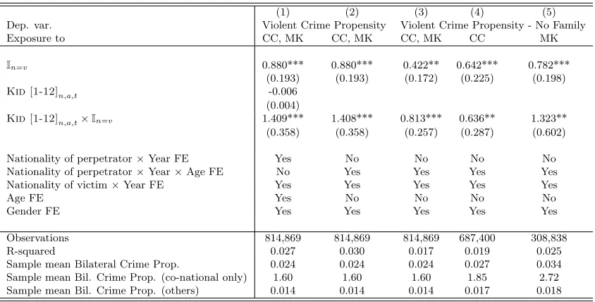
is purely based on human capital depletion and economic deprivation. Making use of
informa-tion on the nainforma-tionalities of both perpetrators and victims, we estimate a bilateral crime regression
documenting violence toward specific nationalities. Crucially, such a bilateral specification makes
possible the inclusion of cohort fixed effects, resulting in the statistical inference being purely based
on bilateral characteristics. The results show that the over-propensity to target victims from their own nationality is more than doubled for cohorts exposed to conflict during childhood. This is
con-sistent with theories of war recurrence stressing the role of persistence in intra-national grievances
and hostility.
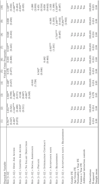
Finally we exploit the fact that Switzerland is a federal state with large variations in institutions
and public policies across its 26 cantons. Our question of interest is whether there exists some
set of integration policies that can mitigate the risk of increased criminality for conflict exposed individuals. Our main finding is that offering labor market access to asylum seekers can strongly
reduce the effect of conflict exposure. In particular, in the presence of the unlimited opportunity
to apply rapidly for jobs in all sectors the violence premium of past conflict exposure drops from 40 percent to 15 percent. Combined with a policy of renouncing to salary deduction, the open job
access even completely removes the crime-increasing effect of conflict exposure. Note that due to
the absence of a randomization scheme in the implementation of policies at the canton-level, our exercise of policy evaluation can barely go beyond correlations. Though limited, this preliminary
public policies can tackle the recurrence of violence in the aftermath of conflict. Besides being of
academic interest, the question of what factors could make immigrants crime prone is also of big societal importance. In many developed Western countries this topic fuels heated and politically
loaded debates, triggering the rise of populist parties. In this respect, one policy relevant conclusion
of the current paper is that the crime risk of asylum seekers with conflict background can be very strongly reduced by putting in place public policies that offer opportunities, and at the same time
get the incentives right for law-abiding behavior.
The remainder of the paper is organized as follows. Section 2 contains the review of the related literature, and section 3 presents the data. Section 4 explains our identification strategy, deals with
the exogenous allocation of asylum seekers in Switzerland, and displays our baseline results, as well
as a battery of robustness checks. Channels of transmission are studied in section 5. Section 6 analyzes the role of public policies and Section 7 is concerned with external validity and applies
the analysis to the much larger group of economic migrants. Finally, Section 8 concludes.
2
Literature Review
Since the pioneering work of Becker (1968), the literature on the economics of crime has studied
a variety of salient covariates of criminal behavior,2, but the nexus between migration and crime
has only received limited attention. Notable exceptions are the papers by Bianchi et al. (2012)
who study the relationship between immigration and crime across Italian provinces, by Bell et al.
(2013) who study the impact of two waves of immigrants to the UK, and by Butcher and Piehl (1998) who study whether the proportion of immigrants who choose to move to particular US cities
affects crime rates. However, in these countries migrants are able to self-select their location, and
the available data is much less fine-grained than in Switzerland.
Also the literature on the effect of war experience has grown in recent years. On the theoretical
front, Rohner et al. (2013) build a model of vicious cycles of war experience leading to low
inter-group trust and hence less inter-inter-group interactions, which in turns results in a higher likelihood of future violence. There is also a growing empirical literature focusing on the effects of war experience
on education, health, collective action and trust.3 Particularly relevant for our current paper is the
literature on the persistence of violence. In particular, Miguel et al. (2011) find a strong positive relationship between the extent of civil conflict in a player’s home country and his propensity
2
Prominent topics in this literature include the role of police activity (Levitt, 1997; Kelly, 2000; Di Tella and Schargrodsky, 2004; Draca et al., 2011) the impact of poverty and inequality (Kelly, 2000; Fajnzylber et al., 2002), the effects of unemployment and recessions ( ¨Oster and Agell, 2007; Fajnzylber et al., 2002; Foug`ere et al., 2009), the impact of mineral discoveries (Couttenier et al., 2014) and the role of illegal drugs (Grogger and Willis, 2000) and urbanization (Glaeser and Sacerdote, 1999).
3
to behave violently on the soccer field, as measured by yellow and red cards. These findings
are consistent with either a violent legacy of war experience, or alternatively with the existence of unobserved country-level characteristics such as for example cultural norms that jointly affect
the war risk and individual violence proneness. Related to this, Grosjean (2014) argues that the
“culture of honor” (enforcing violent vendetta) that was widespread in the Scottish and Scottish-Irish communities in the highlands was “imported” into the US by migrants from these regions in
the 18th century. She shows that this violent culture has only persisted until today in the South
of the US where institutions were weak at the time of migration.
There is also a literature that focuses on the impact of exposure to various events during
childhood. The psychology literature finds a particularly large vulnerability to war trauma for
children aged between 5 and 9 years, as they still lack consolidated identities (see Garbarino and Kostelny, 1996; Kuterovac-Jagodic, 2003; Barenbaum et al., 2004). Beyond the effects of war
exposure, Giuliano and Spilimbergo (2013) find a persistent effect of having experienced a recession
when young on individual beliefs that success in life depends more on luck than effort, support of more government redistribution, and tendency to vote for left-wing parties. In contrast, Gould et
al. (2011) exploit random variation in the living conditions of Yemenite children who arrived in
Israel in 1950 to identify a beneficial impact of a “modern environment” during early childhood (0-5 years of age) on various socio-economic outcomes later in life. Using a quasi-random assignment
of refugees in Denmark, Damm and Dustmann (2014) find that the share of young criminals in a given neighborhood in a given assignment year increases the probability of a young man to commit
a crime later in life and that this effect is especially strong for those from the same ethnic group.
There is also experimental evidence that the formation of pro-social preferences, and in particular of preferences related to altruism, egalitarianism, meritocracy and envy, is particularly active before
12 years of age, and in particular between 6 and 12 years of age (Almas et al., 2010; Bauer et al.,
2014; Bauer et al., 2015; Fehr et al., 2008; and Fehr et al., 2011).
Finally, our paper is also related to the literature on the economics of immigration (cf. e.g.
Borjas, 1994, 2003; Card, 1990, 2001; and Dustmann and Kirchkamp, 2002) and the strain of work
exploiting exogenous allocation of migrants to study labor market outcomes (Edin et al, 2003, Glitz, 2012) and schooling (Gould et al., 2002).
Our paper is novel with respect to various dimensions: First, it is to the best of our knowledge
the first paper that studies the effect of conflict exposure on crime later in life. Second, we can draw on fine-grained data on nationalities of perpetrators and victims to document the persistence
of intra-national hostility. Third, the federalist organization and institutional heterogeneity of
Switzerland allows us to study the impact of public policies on the persistence of violence.
3
Data and Descriptive Statistics
Statistical Office in 2012 about 23.3% of the population were foreign nationals. The number of
asylum seekers – who are defined as individuals who have applied and are waiting for being approved the refugee status – is considerably smaller: Over the 2009-2012 period the yearly average of asylum
seekers was around 30’000 individuals, corresponding to about 0.4% of the Swiss population. Most
of these individuals originate from countries experiencing wars, genocides, political instability, and autocracy. The Swiss federal administration sets stringent conditions for the delivery of political
asylum. In particular, individuals must demonstrate that a return to their home country would
endanger their lives, and economic deprivation cannot be the official reason for requesting asylum to the Swiss administration. As a result, on average only 15 percent of asylum seekers obtain the
asylum. The average processing time of the procedure of asylum request is around 300-400 days.
Appendix C provides more details on the procedure of admission.
Our baseline sample consists of asylum seekers only, observed during their procedure of asylum
request. This is a relatively homogeneous population with similar incentives and characteristics.
We deliberately avoid to compare criminality of asylum seekers to the one of native residents, as this comparison could be driven by unobserved heterogeneity and detection policies biased towards
specific groups. In fact, the identifying variation that we use is the comparison of violent crime
propensities between asylum seekers with past exposure to conflict versus those without exposure.
3.1 Asylum Seekers, Economic Migrants and Conflicts
Data on Asylum Seekers and Economic Migrants. The Federal Office for Migration (FOM)
provides us with non-publicly available administrative individual-level data for all asylum seekers and economic migrants arriving in Switzerland from 1992 onwards. For every person we know the
beginning and end of stay, the location, nationality, age, gender, and the residence status (the
permit held).4 Table 1 displays some descriptive statistics on the population of asylum seekers (for
economic migrants, see Section 7). As expected, the sample is not balanced in terms of gender and
age. With 75% of males and 58% below 30 year old, young males -who are known for being the
most violence prone individuals- are clearly over-represented among asylum seekers. Table 1 lists also the top ten countries of origin. Almost a third of individuals originate from either Eritrea, Sri
Lanka or Nigeria.
Data on Past Exposure to Conflicts. Data on various forms of past exposure to conflict
are used to construct our main explanatory variables. For exposure to civil conflict we retrieve
information from UCDP/PRIO’s “Armed Conflict Dataset” (UCDP/PRIO, v4-2013), which is by
4The main Swiss residence permits are the following. For EU/EFTA citizens there exist the ”L EU/EFTA permit”
Table 1: Share of Asylum seekers in Switzerland by Age, Country of Origin and Gender
Age Class Share Age Class Share
[16-17] 3.11 [45-49] 2.94
[18-20] 10.89 [50-54] 1.61
[21-24] 19.73 [55-59] 0.92
[25-29] 24.78 [60-64] 0.57
[30-34] 18.22 [65-69] 0.27
[35-39] 10.70 [70-79] 0.25
[40-44] 6.00 [80+] 0.03
Country Share Country Share
Eritrea 13.01 Tunisia 4.78
Sri Lanka 9.09 Serbia 4.33
Nigeria 8.57 Turkey 4.26
Afghanistan 5.33 Iraq 4.15
Somalia 5.10 Syria 3.92
Gender Share
Male 75.08
Female 24.92
far the most widely used data on civil conflict. We include all civil conflicts reaching UCDP/PRIO’s
threshold of at least 25 battle-related fatalities. For exposure to mass killings we rely on the most
widely used dataset on mass killings, collected by the “Political Instability Task Force” (Political
Instability Task Force, 2013). They define mass killings as events that “involve the promotion,
execution, and/or implied consent of sustained policies by governing elites or their agents – or in the case of civil war, either of the contending authorities – that result in the deaths of a substantial
portion of a communal group or politicized non-communal group”.5 Note that exposure to mass
killings of civilians is a very different type of violence exposure than the one for civil war. An event is only coded as civil war when fighting is two-sided and when battle-related casualties are
sizable for all conflict parties. In contrast, mass killings of civilians are one-sided with civilians
being helpless victims, and fighting not necessarily being related to battles. Hence, in many cases mass killings can take the form of purges by the state against civilians rather than armed conflict
between the state and armed rebels.
Our data on asylum seekers report no information on exposure to violence during conflict at the individual-level. Therefore we make the choice of measuring past conflict exposure at the
cohort-level. Our baseline measure is Kid [1-12], a binary variable that codes for cohorts who
were aged between 1 and 12 when civil conflict or mass killing occurred in their origin country.
Notice that this cohort effect encompasses direct and indirect forms of exposure to conflict that
we cannot disentangle, such that being personally targeted by acts of violence (e.g. being injured or witnessing the killing of a family member) or being exposed to a war context where economic
deprivation and social capital depletion prevail. We focus on the first 12 years of age, in line with
the substantial evidence that many preferences and attitudes are formed during this period of life.6
Moreover, beyond its intrinsic interest, focusing on exposure to violence during childhood serves
the purpose of causal analysis by alleviating endogeneity issues due to self-selection into violence,
e.g. excluding former perpetrators (see Section 4.1). Finally, in some specifications, we split our
variable of exposure into two categories, Kid [1-12] (only cc)and Kid [1-12] (only mk), that
5
By this definition, killing episodes have in the last 50 years taken place in 28 different countries, and include all of the most notorious historical instances of large-scale massacres like, for example, the ones in Sudan, Rwanda, Bosnia or Cambodia.
6Garbarino and Kostelny, 1996; Kuterovac-Jagodic, 2003; Barenbaum et al., 2004; Fehr et al., 2008; Almas et al.,
correspond respectively to specific exposure to Civil Conflict and Mass Killing. In our robustness
analysis, we also build an alternative measure of victimization at the cohort-level,Women[1,+], a
binary variable coding for cohorts of women who experienced (at any age) a conflict with systematic
wartime rape in their origin country. To this purpose we use the data of Cohen (2013). She takes as
starting point the list of major wars of Fearon and Laitin (2003) and uses a variety of data sources to determine which of these wars feature the systematic use of wartime rape by governments or
insurgents.
3.2 Crime Data
The Federal Statistical Office (FSO) provides us with non-publicly available exhaustive data on all
crimes detected by the police in Switzerland between 2009 and 2012. This individual-level dataset
has been collected by local police services and covers all cases when somebody was charged with infractions to the (federal) Penal Code. Remarkably, the data convey precise information on the
nationalities and residency status of victims and perpetrators of any detected crime, as well as on
the place, time and type of the crime. Following the empirical literature crimes are sorted into two broad categories: violent crime (murders, injuries, threats, sexual assault...) and property
crime (thefts, burglaries, robberies, scams...). Our main focus is on violent crimes perpetrated
by asylum seekers. In the baseline analysis we make no distinction in term of nationalities or background of victims. This makes sense given that, in the data, violent asylum seekers target not
only other asylum seekers but also the rest of the population: 35% of victims are themselves asylum
seekers, 28% are foreign residents, 36% are natives. However intra-asylum seeker violence is clearly over-represented and victim targeting is not random –a pattern at the core of the mechanism we
investigate in Section 5.2.
For the sake of confidentiality the FSO prevents us from merging at the individual level crime data with migration data. Together with this legal provision, the fact that our explanatory variables
of past exposure to violence are anyway measured at the cohort-level, leads us to conduct our
statistical analysis at the level of a cohort of asylum seekers from nationalityn, genderg, age group
a, in year t. Hence, combining migration and crime datasets at the cohort-level, we build our
main dependent variable, the violent crime propensity, labeled CPn,g,a,t, that corresponds to the
yearly number of crimes perpetrated by a cohort divided by its size.7 Note that, in our definition
of a cohort, we lump together individuals by age brackets rather than by year of birth brackets
because age is a first-order determinant of criminality.8 Given the short time span of our panel
(2009-2012), these two coding options are in fact very close and they would be identical in the case of a cross-sectional dataset.
7
This definition of a cohort-specific crime propensity is not affected by recidivism, as we count the number of crimes committed by different individuals (i.e. if person A commits two crimes and person B of the same cell none, this results in the same overall crime propensity as when both of them commit one crime each).
8
Exhaustive data of such high quality is only available in Switzerland for detection data of
charges for crime, and not for data on final convictions by a court.9 While of course the number of
charges for crime are highly correlated with the number of convictions, there may be discrepancies
if for example in some cantons and years the police authorities are more active and successful than
in others. Such spatial differences in detection probabilities of a crime are however accounted for by the exogenous allocation of asylum seekers across the Swiss territory (or the inclusion of canton
× year fixed effects in Section 7). There could also be a wedge between crime rates of nationals
and foreigners if for example some police forces were to predominantly control foreign-looking individuals. This however would not bias our estimation as we restrict ourselves to within-asylum
seeker comparisons and do not compare asylum seeker crime rates with crime rates of Swiss citizens.
3.3 Descriptive Statistics
We observe a total annual number of between 22790 and 32413 asylum seekers from 134 nationalities
over the 2009-2012 period. After aggregating by nationalityn, genderg, age groupa, for each yeart,
this leaves us with 4820 cohorts, which are our units of observation. The average cohort is composed of 22 individuals. Notice that the variance in cohort size is large (standard deviation equals 63
individuals) and this feature of our micro-data calls for weighting our cohort-level regressions by
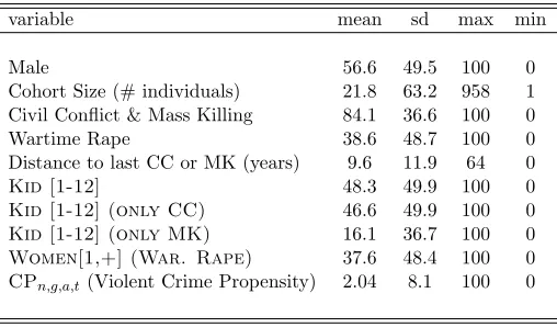
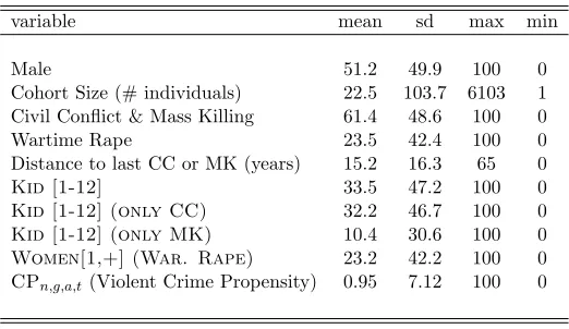
the number of individuals in each cohort (see our discussion on grouped data in Section 4). Table 2 reports the main descriptive statistics for cohorts. Note first that 84% of cohorts
originate from countries that have experienced at least one episode of civil conflict or mass killings
since 1946. Among the 134 nationalities of origins, conflicts occurred in 90 countries, mass killings in 27 countries, and wartime rape in 46 countries. These nationalities are the ones that contribute
to our identifying variations. All these countries experienced violence in some, but not all years,
leading to within-nationality, inter-cohort variations in exposure to violence: The sample mean
of childhood exposure, Kid [1-12], is equal to 48%. As for our alternative measure of exposure,
Women[1,+], we see that 38% of female cohorts have experienced a conflict where wartime rapes
were pervasive. Finally, note that a substantial part of asylum seekers do not flee their country
during war time, but years or even decades afterwards.10 The average number of years since the
last Civil Conflict/Mass Killing is around 10 years.
We now turn to cohort-level (violent) crime propensities. The sample average of CPn,g,a,t
is equal to 2.04% with large heterogeneity across cohorts (s.d. equals 8.1%), the main sources
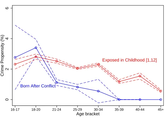
of variance being related to age. Figure 1 explores the age-crime nexus by reporting average
propensity by age bracket for the two groups of cohorts at the core of our identification strategy:
9Due to the differences across cantons regarding the judicial procedures and duration of trials, the harmonization
of individual conviction data is very hard and does not currently exist. Moreover, a meaningful harmonization of conviction data for asylum seekers would be even harder, as in many cases asylum seekers may get expelled before the end of the lengthy trial.
10
Table 2: Cohorts of Asylum Seekers - Summary Statistics
variable mean sd max min
Male 56.6 49.5 100 0
Cohort Size (# individuals) 21.8 63.2 958 1
Civil Conflict & Mass Killing 84.1 36.6 100 0
Wartime Rape 38.6 48.7 100 0
Distance to last CC or MK (years) 9.6 11.9 64 0
Kid [1-12] 48.3 49.9 100 0
Kid [1-12] (only CC) 46.6 49.9 100 0
Kid [1-12] (only MK) 16.1 36.7 100 0
Women[1,+] (War. Rape) 37.6 48.4 100 0
CPn,g,a,t(Violent Crime Propensity) 2.04 8.1 100 0
Note: Sample of 4820 cohorts of asylum seekers, 134 nationalities, 14 age brackets, 2009-2012. Except for cohort size and distance to last CC or MK, all figures represent percentages.
Cohorts exposed to CC or MK during childhood (in red) and those born after conflict (in blue).11
For the two groups, we see a clear spike in violent crime in early adulthood and then a steady
decrease across ages. Pattern and magnitude conform to the large evidence on age-crime curves that has been collected in the criminology literature for other populations-periods (see Freeman,
1999, for a review on determinants of criminal behavior).
The striking and novel point here relates to the crime differential between the two groups: While for very young cohorts the crime propensity is high for any of the two groups, from the age
of 20 on an important gap widens up. In particular, cohorts with past exposure to conflict keep
having high crime propensities until the age of around 40, while for cohorts born after conflict, the crime propensity drops already massively from age 21 onwards. After the age of 40 the two curves
converge again on a low level. Across the considered age brackets, the average differential is equal
to 0.85 percentage points, a substantial wedge that implies that cohorts exposed during childhood are on average 1.75 times more prone to violent crimes than cohorts born after a conflict. This
graphical evidence illustrates our main result. The econometric analysis aims to confirm that this
excess crime propensity is causally related to the exposure to violence in childhood, accounting for a variety of potential confounding factors.
4
The Impact of Past Exposure to Conflict on Violent Crimes
The first step of our empirical analysis documents the causal impact of past exposure to conflict
on violent crimes. Section 5 deals with the potential mechanisms at work.
11
We restrict ourselves to the subsample of cohorts from countries with conflict or mass killings background that are born after war or exposed during their childhood (Kid [1-12]= 1). For each age class we averageCPn,g,a,tacross
Figure 1: Age-Violence Curves
Exposed in Childhood [1,12]
Born After Conflict
0
2
4
6
Crime Propensity (%)
16-17 18-20 21-24 25-29 30-34 35-39 40-44 45+
Age bracket
Confidence intervals are set at 99%.
4.1 Identification Strategy
Our unit of observation is a cohort. The decision to perpetrate a crime or not is however made
at the individual level. A specification based on micro-data would have the individual as unit of observation and would estimate a random-utility discrete-choice model, such as e.g. a binomial
logit. For samples based on grouped data, like ours, Durlauf et al. (2010) show that the logit
model translates into a linear specification where the dependent variable is the log of the odds ratio of the crime propensity. They recommend to implement this aggregate logit procedure only
when the aggregation-level is sufficiently high such that sampling errors are limited and group-level
crime frequencies approximate well the underlying crime probabilities. In our context, the average cohort size is not large (i.e. 21 individuals) and, more importantly, the variance is large, with
many small cohorts –the ones with 5 individuals or less representing 59% of the sample. Hence, sampling errors become a salient issue and, together with the fact that crime is a rare event, this
implies that the number of zeroes is very large (CPn,g,a,t = 0 for 82% of cohorts), making the
computation of odds ratio problematic. We consequently prefer a baseline specification that is
compatible with zeroes (and ones as well) by estimating a linear crime regression withCPn,g,a,t as
dependent variable. This choice follows the standard practice in the crime literature (see e.g. Bell
et al., 2013). Notice that all our cohort-level regressions are frequency-weighted by the size of the cohort as recommended by Angrist and Pischke 2009 (Section 3.4.1, pp. 91-94) in the context of
grouped data. As a consequence we report inflated sample size in all regressions. Finally, in the
Our baseline crime regression corresponds to
CPn,g,a,t =α×Kid [1-12]n,a,t+ k=80+
X
k=13
β(k)×expo(k)n,a,t+FEn,t+FEg+FEa+εn,g,a,t, (1)
whereCPn,g,a,tstands for the violent crime propensity of a cohort of nationality (n)×gender(g)×
age bracket (a)×year (t). As discussed above, our main explanatory variable isKid [1-12]n,a,tthat
is a binary measure of childhood exposure. The set of control variablesexpo(k)n,a,tare also binary
variables coding for past exposure, but at the later agesk∈ {13,14,15, ...,80+}. Hence, in equation
1, the implicit reference group consists of cohorts born after a conflict.12 As a consequence, our
parameter of interestαcan be interpreted as the crime differential between cohorts exposed during
their childhood and cohorts born after the conflict. Crucially, the richness of our dataset makes
possible the inclusion of a vast array of fixed effects that account for unobserved heterogeneity in
nationality×year (FEn,t), in age (FEa) and in gender (FEg). Finally, robust standard errors are
clustered at the nationality×year level. We discuss now in more details the potential econometric
pitfalls.
Spatial sorting in Switzerland – A first challenge relates to the fact that crime-prone individuals tend to self-select into a crime-facilitating environment. For example, individuals
exposed to conflict in their origin country are used to live in areas with high economic
depri-vation and violence; by contrast, individuals from peaceful background, once in Switzerland, could strategically avoid criminal hotspots or poorest neighborhoods with few labor market
opportunities. This example illustrates a case where past exposure to conflict correlates with
an unobserved cohort characteristic (i.e. preferences in terms of living area) that impacts crime-proneness in Switzerland.
Our empirical strategy is able to rule out this spatial sorting issue by restricting our core estimates to asylum seekers, a subsample of migrants who are exogenously allocated across
Switzerland (see Section 4.2). Notice that this exogenous allocation has a second virtue
related to the fact that cantons are very heterogeneous in term of pro-asylum policies which may affect the elasticity of violence propensity to past conflict exposure. The exogenous
allocation makes sure that exposed individuals cannot select location according to cantonal
policies.
Pre-conflict characteristics of origin countries – Our empirical analysis intends to
cap-ture theconsequences of past conflict exposure on crime propensity. We consequently include
nationality fixed effects (captured byFEn,t), in order to filter out slow-moving characteristics
of the origin country that could correlate with frequent war outbreaks and crime-promoting
characteristics (weak institutions, low social capital and dismal inter-ethnic trust, etc.).
12We code
expo(k)n,a,t= 1 for cohorts who were agedkyears old when civil conflict or mass killings occurred in
Selection into migration – The push and pull factors determining migration decisions
are likely to be affected by conflicts. Presumably, peacetime is associated to economic mi-gration while humanitarian migrants are over-represented in post-conflict periods. In turn,
this could affect post-migration crime incentives in the destination country. The inclusion
of gender and age bracket fixed effects, FEg and FEa, aims to control for the main
socio-demographic co-determinants of violent behaviors and the decision to emigrate. Further, at
least as important is the inclusion of the nationality×years fixed effects (FEn,t) which absorb
time-series variations in origin-specific push factors.
Note that we have no information on the educational level of asylum seekers. Therefore
the estimated excess criminality of exposed cohorts could be partly linked to unobserved heterogeneity in human capital. In our baseline specifications we do not want to control for
this channel because we believe that economic deprivation and educational disruption are
important drivers of the causal impact of past exposure to conflict on violent criminality. However, when we study the specific channel of intra-national grievances in Section 5.2 we
control for education and human capital thanks to the inclusion of cohort-specific fixed effects
(in bilateral crime regressions).
Perpetrators and victims – Related to the previous point, it could be that after a con-flict perpetrators are over-represented among migration waves. Hence, high crime proneness
in Switzerland may not only be due to participation to the war, but to prewar individual
disposition. To alleviate this concern we exclude the potential perpetrators by focusing on the sub-sample of victims exclusively, i.e. i/ individuals who were children during the war
compared to those born afterwards; ii/women born before the war compared to those born
afterwards.
All in all, we deal with a demanding empirical strategy: Our source of identification corresponds
to variations in crime-propensities across cohorts of asylum seekers from the same nationality,
gender and migration wave but with different exposure to conflict (i.e. born after war/exposed in childhood). Because these cohorts inevitably differ in terms of age, we must control for the
direct effect of age by comparing them to other cohorts with similar age structure but non-exposed backgrounds (e.g. coming from peaceful countries or born after conflict in another country). To
give an example, our strategy consists of computing the crime differential of two Rwandese, one
born in 1996 (born after the 1994 genocide), and one born in 1990 (exposed during childhood), migrating to Switzerland in 2012. In order to control for crime-age effects, their crime differential
is compared to the one of two Nigerians of same ages –born in 1990 and 1996– but with peaceful
background (both are born after the 1967-1970 civil war). Our comparison of the blue and red crime-age curves in Figure 1, panel (a), follows the same logic.
Thus, our strategy is basically akin to a difference-in-difference in country × cohort. The
after. A threat to our identification strategy would be that, for a given nationality or age or gender,
the federal administration allocates asylum seekers across centers according to their exposure to conflict during childhood in their home country. With this respect, statistical tests of the exogenous
allocation in Table 20 show thatKid [1-12]cannot explain the cross-cantonal allocation of asylum
seekers (see Section 4.2). Another reassuring pattern in our data is the observation in Table 5 of a sharp decrease in crime propensity between cohorts born during conflicts and those born just
after. Finally, we explore further the plausibility of our identifying assumption in Section 4.4.
Among other validity checks, we perform a Monte Carlo (placebo) test based on cross-cohorts counterfactual reassignments of conflict exposure during childhood.
4.2 Exogenous Spatial Allocation of Asylum Seekers in Switzerland
We now provide an overview of the actual process of allocation of asylum seekers across Swiss cantons. We also discuss briefly some statistical evidence supporting the view that the distribution
key is based on canton population size only and is exogenous to migrants’ characteristics. Many
more details on the institutional/legal aspects and on the formal statistical tests are provided in Appendices C and D respectively.
Overview of the allocation process–Most asylum seekers enter Switzerland illegally (especially crossing the Italian border) and apply for asylum in one of the four national reception and procedure
centers (RPC). In the RPC, asylum seekers go through interviews, where they are asked to provide
identity proofs, fingerprints, and their application reasons. During the lengthy assessment process, the credible asylum seekers are granted a temporary N permit by the Swiss authorities. Given
the difficulty in assessing the threat of persecution in the home country and the large number of
applicants (around 25 000 per year over the 2009-2010 period), the asylum process takes substantial time. Between 2009-2010, the average duration of the process was 300-400 days, with complex cases
taking several years.
Crucially, during this period holders of the N-permit are exogenously allocated to cantons and are not allowed to change canton. The allocation of new N-permit holders to the 26 Swiss cantons is
determined by a exogenous allocation key based on the cantonal population. Once an asylum seeker
has been allocated to a given canton, the canton in charge organizes the accommodation in cantonal centers or flats and takes care of the interviews and of financial matters. This allocation rule was
introduced in the amendment to the Aliens Law in 1988, presumably to minimize self-segregation
and ghetto effects and avoid social tensions between natives and asylum seekers.
The allocation is made by the Federal Office for Migration in Bern and its decision cannot be
appealed unless under certain precise conditions (family unity reasons like minors being allocated to a different canton than their parents or if the asylum seeker or a third person are under serious
threat) and the change of the canton is possible only if the two cantons approve it. According to
Statistical Evidence–Figure 2 in the Appendix displays the time series evolution of asylum seeker stocks across the 26 Swiss cantons between 1994-2010 (the main peak corresponding to the end
of the Kosovo war). Visual inspection confirms parallel trends across cantons and this constitutes
a first and rough piece of evidence consistent with an exogenous allocation process of migrants across cantons. More substantially, we provide formal statistical tests in Table 20 of Appendix D.
The purpose is to tackle the question of whether there is indeed an exogenous allocation of asylum
seekers following the official population-based distribution key –as we claim– or if there may be some selection on relevant dimensions. The basic approach consists in testing for the difference
in means between cantons for various observable cohort characteristics (i.e. exposure to violence
during childhood, age, gender). We first perform this test for each nationality of asylum seekers. However, a concern is that, for small nationality sizes, sampling variations mechanically lead to
observed patterns of spatial concentration in some cantons. A first attempt to tackle this sampling
issue consists in pooling cohorts from all nationalities by year. A second attempt corresponds to a Monte Carlo simulation (1000 draws) generating artificial random allocations that we compare to
the observed allocation. Overall, the tests of Table 20 are supportive of our identifying assumption
that the allocation of asylum seekers across cantons can be considered as exogenous with respect to their age, gender and past exposure to violence.
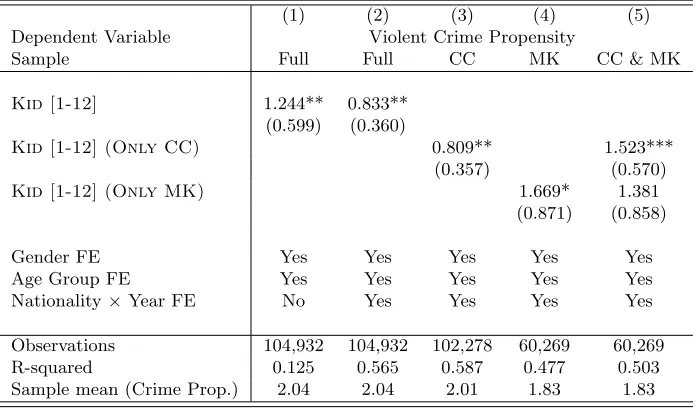
4.3 Baseline Results
Table 3 displays the baseline estimation results of our cohort-level crime regression (equation 1).
We report only our coefficient of interest,α, that captures the impact on violent crime propensity
of cohorts exposed to civil war or mass killings during childhood (1-12 years), the reference group
being cohorts born after conflict. Column 1 reports the results of a pooled regression with age
and gender fixed effects but without country × year fixed effects. The coefficient of interest is
positive and significant at the 5 percent threshold. However, as explained in Section 4.1 this
correlation is potentially driven by confounding factors that relate to pre-conflict characteristics of origin countries or by selection into migration. In Column 2, we consider a specification with
the full battery of fixed effects where the identifying variations come from within-nationality /
between-cohorts comparison. This is our preferred specification (baseline). The coefficient of past exposure is reduced by one third but it retains statistical significance and a positive sign. In term
of magnitude, we observe that the crime propensity of cohorts exposed during childhood is on
average 0.83 percentage points higher than the propensity of their co-national cohorts born after
the war –a substantial effect given that the sample mean of violent crime propensity is equal to
2.04 percentage points. By means of benchmarks, gender and age have comparable consequences on
crime propensity. The non-reported coefficient of the male dummy (reference group being female) is
3.03. This is not surprising, as it is widely known that most violent crimes are perpetrated by men.
16-17 years old have 6.5 percentage points, the 18-20 years old have 5.95 percentage points, 21-24
years old 4.8 percentage points and 25-29 years old 3.5 percentage points higher crime propensity
than the cohort being more than 50 years old. In a nutshell, even if gender and age tend to be
powerful determinants of crime, past exposure to conflict in childhood still substantially matters.
In columns 3 and 4 we run the same specification as in column 2, but now separately for conflict and mass killings. To focus on within-nationality variations, the sample is restricted to countries
having experienced each specific type of violence. Column 5 includes simultaneously the two
mea-sures of past exposure. While the coefficients of interest are in both cases positive and of similar magnitude, only the impact of CC is statistically significant, while the coefficient of MK narrowly
misses conventional significance thresholds.
Table 3: Benchmark Regression of Crime Propensities and Conflict Exposure
(1) (2) (3) (4) (5) Dependent Variable Violent Crime Propensity
Sample Full Full CC MK CC & MK
Kid [1-12] 1.244** 0.833**
(0.599) (0.360)
Kid [1-12] (Only CC) 0.809** 1.523***
(0.357) (0.570)
Kid [1-12] (Only MK) 1.669* 1.381
(0.871) (0.858)
Gender FE Yes Yes Yes Yes Yes Age Group FE Yes Yes Yes Yes Yes Nationality×Year FE No Yes Yes Yes Yes
Observations 104,932 104,932 102,278 60,269 60,269 R-squared 0.125 0.565 0.587 0.477 0.503 Sample mean (Crime Prop.) 2.04 2.04 2.01 1.83 1.83
Note: OLS estimations weighted by the number of individuals in each cohort. Robust standard errors are clustered at nationality×year levels. *** p<0.01, ** p<0.05,* p<0.1. All estimations include gender fixed effects, age group fixed effects and a set of binary variables coding for past exposure, but at the later agesk∈ {13,14,15, ...,80+}. The group of reference is people born after the last years of violence. The dependent variableViolent Crime Propensity stands for the violent crime propensity of a cohort of nationality (n)×gender(g)×age bracket (a)×year (t). Kid [1-12] is a binary measure of childhood exposure to civil conflict or mass killing (columns 1 and 2), to civil conflict only (column 3), to mass killing (column 4). For columns 3 to 5, the sample is restricted to countries having experienced each specific type of violence during childhood.
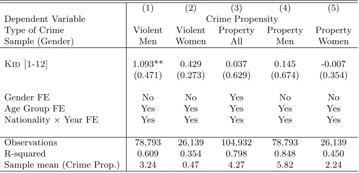
Heterogeneous Effects: Gender and Type of Crime – In Table 4 we study heterogeneous
effects with respect to gender and type of crime. Columns 1 and 2 replicate our baseline specifica-tion (Column 2 of Table 3) on the subsamples of male and female cohorts respectively. The results
are clearly driven by men, with the coefficient for women being of smaller size and not statistically
magnitude and the statistical significance of our variable of interest is strikingly lower, suggesting
that exposure to conflict during childhood impacts future violent behaviors, but leaves future non-violent criminality unaffected. We see this contrasted evidence as a first indication that our causal
effect captures a mechanism of perpetuation of violence –a point that we develop in more detail in
Section 5. From the perspective of causal analysis we interpret the absence of effect for property crime as an indication that the correlation between past exposure and violent crime is unlikely
to be spuriously driven by omitted factors (unless such factors were to affect differentially violent
crimes and property crimes).
Table 4: Heterogeneous Effects – Gender and Type of Crime
(1) (2) (3) (4) (5) Dependent Variable Crime Propensity
Type of Crime Violent Violent Property Property Property Sample (Gender) Men Women All Men Women
Kid [1-12] 1.093** 0.429 0.037 0.145 -0.007
(0.471) (0.273) (0.629) (0.674) (0.354)
Gender FE No No Yes No No
Age Group FE Yes Yes Yes Yes Yes Nationality×Year FE Yes Yes Yes Yes Yes
Observations 78,793 26,139 104,932 78,793 26,139 R-squared 0.609 0.354 0.798 0.848 0.450 Sample mean (Crime Prop.) 3.24 0.47 4.27 5.82 2.24
Note: OLS estimations weighted by the number of individuals in each cohort. Robust standard errors are clustered at nationality×year levels. *** p<0.01, ** p<0.05,* p<0.1. All estimations include gender fixed effects, age group fixed effects, nationality×year fixed effects and a set of binary variables coding for past exposure, but at the later agesk∈ {13,14,15, ...,80+}. The group of reference is people born after the last years of violence. The dependent variableViolent Crime Propensity stands for the violent (property) crime propensity of a cohort of nationality (n)×
gender (g)× age bracket (a)× year (t) in columns 1 and 2 (columns 3 to 5). Kid [1-12] is a binary measure of childhood exposure to civil conflict or mass killing.
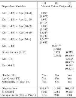
Heterogeneous Effects: Age – Table 5 is also devoted to heterogeneous effects, with a special
focus on age. In Column 1, we are interested in lifecycle modulations of the impact of past exposure. We interact our main explanatory variable with (mutually exclusive) decade dummies coding for
the current age of the cohorts. We see no significant difference for exposed and non-exposed
people aged below 40, while the gap is positive and statistically significant for older cohorts. These results confirm the insights of Figure 1 where unconditional crime propensity peaks during teenage
years and then decreases drastically for non-exposed cohorts while it remains at a high level for
exposed cohorts. Our interpretation is that past exposure to conflict during childhood prevents the dampening effect of age on violence to take place.
In the next two columns we investigate in more details the age where exposure to conflict
takes a value of 1 if there has been a civil conflict or a mass killing in the 12 yearsbefore being born.
If the main effect of conflict exposure is about economic deprivation or institutional collapse, we
should expect the variableBorn After [0-12]to be a similarly powerful predictor as our variable
of interest. It turns out that this is not the case and we get back to this issue when we study the
underlying mechanisms (Section 5). In fact, while our main explanatory variable of past exposure
retains its magnitude and statistical significance, the coefficient ofBorn After [0-12]is of much
smaller magnitude and is not statistically significant at conventional levels. This sharp decrease
in crime propensity for cohorts born just after the war with respect to those exposed during their childhood is again reassuring for our causal analysis as it makes unlikely any contamination of the
results by omitted variable bias. In column 3, Kid [1-12] is split in two, with a separate variable
capturing the impact of war exposure during the first five years of life, and a second variable cap-turing war exposure during the 6th and the 12th year of life. We find that the effect is stronger
for Kid [1-5]. This is consistent with earlier studies pointing out the crucial importance of these
five earliest years of life (see e.g. Gould et al. (2011) and the literature on early child development (e.g. Heckman et al., 2013)).
Inspired by the recent article by Giuliano and Spilimbergo (2014) we also investigate in Table 14 whether there is an effect of conflict exposure in early adulthood (see Appendix). There are
two main reasons why this age bracket (18-25 years of age) is less suitable in our context than in theirs: First of all, as shown in the psychological literature cited above, war trauma has particularly
strong effects in the first years of life. Second, for our identification strategy it is crucial to focus
on conflict victimization to rule out self-selection into violence. While one can plausibly claim that young children below the age of 12 are only victims, this is of course not the case anymore for
the 18 to 25 years old. Still, as shown in Appendix Table 14 our results on the impact of conflict
exposure in the first 12 years of age on violent crime continue to hold when controlling specifically for conflict exposure in the age bracket 18 to 25. While civil conflict exposure of the 18-25 years
old does not affect future crime propensities, the exposure to mass killings in young adulthood does
have an effect. Further, as shown in columns 3 and 4, conflict exposure at ages 18-25 increases the propensity to property crime later in life.
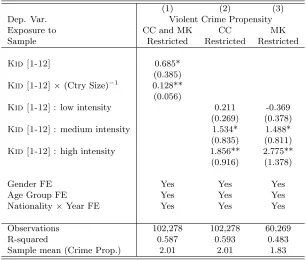
Heterogeneous Effects: Intensity of Conflict – Finally, Table 6 is devoted to the
heteroge-neous impact of past exposure according to the intensity of the conflict in the origin country.13 In
column 1 our main explanatory variable is interacted with the inverse of the country of origin size.
The idea is that the conflict threshold of UCDP/PRIO is defined in terms of the absolute number of fatalities and hence is likely to pick up more minor conflicts in large than in small countries. We
measure size in terms of surface (km2) and not population in order to mitigate any reverse
causa-13Ideally, we would like to exploit both the geographical location of conflict within a country-year and the birth
Table 5: Heterogeneous Effects – Lifecycle Modulation and Age of Exposure
(1) (2) (3) Dependent Variable Violent Crime Propensity
Kid [1-12]×Age [16-20] 0.263
(1.077)
Kid [1-12]×Age [21-29] 0.650
(0.418)
Kid [1-12]×Age [30-39] 0.590
(0.381)
Kid [1-12]×Age [40-49] 1.824**
(0.729)
Kid [1-12]×Age [50+] 1.547**
(0.637)
Kid [1-12] 0.857**
(0.336)
Born After [0-12] 0.125 0.273
(0.381) (0.346)
Kid [1-5] 0.835*
(0.502)
Kid [6-12] 0.484
(0.303)
Gender FE Yes Yes Yes Age Group FE Yes Yes Yes Nationality×Year FE Yes Yes Yes
Observations 104,932 104,932 104,932 R-squared 0.565 0.565 0.565 Sample mean (Crime Prop.) 2.04 2.04 2.04
Note: OLS estimations weighted by the number of individuals in each cohort. Robust standard errors are clustered at nationality×year levels. *** p<0.01, ** p<0.05,* p<0.1. All estimations include gender fixed effects, age group fixed effects, nationality×year fixed effects and a set of binary variables coding for past exposure, but at the later agesk∈ {13,14,15, ...,80+}. The group of reference is people born after the last years of violence. The dependent variableViolent Crime Propensity stands for the violent crime propensity of a cohort of nationality (n)×gender(g)×
age bracket (a)×year (t). Kid [1-12]is a binary measure of childhood exposure to civil conflict or mass killing during childhood. Born after [0-12] takes a value of 1 if there has been a civil conflict or a mass killing in the 12 years
beforebeing born. Kid [1-5](Kid [6-12]) is a binary measure of childhood exposure to civil conflict or mass killing between 1 to 5 years old (6 to 12 years old).
tion bias from conflict intensity to population size. As expected, the coefficient of the interaction
term is positive and significant. Thus, the impact of past exposure is larger for cohorts
originat-ing from small countries. In column 2 we turn to a more accurate assessment of the intensity of past exposure. We construct three mutually exclusive quantiles of conflict intensity, measured as
number of battle-related deaths in a given country-year weighted by the area of the country. For an average area, low intensity corresponds to less than 4333 casualties by country-year, medium
intensity to 4333-43694 and high intensity to more than 43694 casualties. The results show that
mass killings intensity. To construct the three quantiles of intensity, we rely on the country-year
number of deaths index provided by Political Instability Task Force (2013),14 weighted by country
area. Here again the coefficients are ordered very clearly: the largest impact is for highly intense
mass-killings, followed by events of medium intensity, while we detect no impact for mass killings
of low intensity.
Table 6: Heterogeneous Effects – Intensity of Conflict
(1) (2) (3) Dep. Var. Violent Crime Propensity Exposure to CC and MK CC MK Sample Restricted Restricted Restricted
Kid [1-12] 0.685*
(0.385)
Kid [1-12]×(Ctry Size)−1 0.128**
(0.056)
Kid [1-12]: low intensity 0.211 -0.369
(0.269) (0.378)
Kid [1-12]: medium intensity 1.534* 1.488*
(0.835) (0.811)
Kid [1-12]: high intensity 1.856** 2.775**
(0.916) (1.378)
Gender FE Yes Yes Yes
Age Group FE Yes Yes Yes Nationality×Year FE Yes Yes Yes
Observations 102,278 102,278 60,269 R-squared 0.587 0.593 0.483 Sample mean (Crime Prop.) 2.01 2.01 1.83
Note: OLS estimations weighted by the number of individuals in each cohort. Robust standard errors are clustered at nationality×year levels. *** p<0.01, ** p<0.05,* p<0.1. All estimations include gender fixed effects, age group fixed effects, nationality×year fixed effects and a set of binary variables coding for past exposure, but at the later agesk∈ {13,14,15, ...,80+}. The group of reference is people born after the last years of violence. The dependent variableViolent Crime Propensitystands for the violent crime propensity of a cohort of nationality (n)×gender (g)×
age bracket (a)×year (t). Kid [1-12]is a binary measure of childhood exposure to civil conflict or mass killing.
4.4 Robustness Checks
In this section we show that the baseline estimate of Table 3, Column 2 is robust to a battery of
sensitivity checks. All tables are relegated to Appendix A.
Alternative Crime Regressions – We start with testing a different level of clustering as an
14
alternative to the baseline nationality × year level. In Table 13 we replicate the baseline Table
3 with standard errors clustered at the nationality × age level. The coefficients retain statistical
significance at the 5 percent level in all the specifications where the full battery of fixed effects is
included (Columns 2-5).
In Table 15 we consider alternative econometric specifications for the crime regression (see the discussion in Section 4.1). In columns 1-3 we consider three options for dealing with zeroes and
ones in our dependent variable. Column 1 restricts the OLS crime regression to the subsample
of cohorts where crime propensity is strictly between 0 and 1. In spite of the major sample
size reduction, the coefficient retains statistical significance (at the 10 percent level) and similar
magnitude. Column 2 follows a less drastic route by keeping the full sample and estimating a
Tobit model with two censoring levels, at 0 and at 1. The coefficient of interest is still significant at the 1 percent level. In column 3 we estimate a Poisson model on the full sample. This type
of econometric model is well suited for count data like the cohort-level amount of violent crimes.
Here again the coefficient is significant with a magnitude comparable to its OLS counterpart.15
Columns 4 and 5 test for robustness to the removal of outliers. We retrieve from our baseline
specification the estimated residuals. Then we trim the sample to remove all observations for
which the residuals are further away than three standard deviations (column 4) or, even more radically, two standard deviations (column 5) from the mean residual. In both cases we obtain
a statistically significant coefficient at the 5 percent level; its magnitude is reduced with respect to its baseline counterpart. In column 6 we go back to our baseline specification but change the
weighting procedure by considering probability rather than frequency weights. The reported sample
size is not inflated anymore and corresponds to the number of cohorts. Reassuringly, the estimated coefficient and standard deviation are unchanged. Column 7 displays the result for the unweighted
regression. The magnitude of the coefficient is comparable to its baseline value; however, it is much
less precisely estimated. This confirms that small cohorts, where crime propensity is more likely to take extreme values (0 or 1), lead to mismeasurement errors and statistical noise.
Table 16 implements the aggregate logit procedure. It simply consists of an OLS crime
regres-sion where the dependent variable is now the log(odds-ratio) of Crime Propensity, namely ln CP
1-CP.
All other features are identical to the baseline specification. As explained in Section 4.1, coping
with (i) zeroes and ones, and (ii) small cohorts, is problematic in such a setting. In column 1 we
replace byCP= 0.001 and CP= 0.999 the observed values of CPthat are equal to zero and one
respectively. Though ad-hoc, this coding rule allows to force the definition of the odds-ratio for all
cohorts. In columns 2 and 3 the same coding rule is used but we exclude small cohorts from the
sample (respectively less than 2 individual and less than 3 individuals). Column 4 abstracts from
this coding rule by simply excluding all cohorts with CP = 0 orCP = 1 from the sample. This
leads to a big reduction in sample size. Finally column 5 uses probability weights and column 6
dis-plays the result for the unweighted regression. All in all the coefficient of interest keeps its positive
15Note that the estimated standard deviations with the Tobit model have to be considered carefully due to the
sign. Its magnitude is not directly comparable to its baseline value due to the logistic transform of
the dependent variable. The statistical significance is slightly reduced (below 10 percent threshold instead of 5 percent in the baseline).
Placebo Test of conflict exposure during childhood–As mentioned in section 4.1, our iden-tifying assumption is that past exposure to conflict is the only reason why the decline in crime
rates with age is smaller for asylum seekers exposed in childhood than for asylum seekers from the
same nationality and born after the war. With this respect, a reassuring pattern in our data is the observation in Table 5 of a sharp decrease in crime propensity between cohorts born during conflicts
and those born just after. We now go one step further by performing a falsification exercise based
on a randomization of conflict exposure during childhood. More specifically, we follow a Monte Carlo approach where we postulate a data generating process that randomly reassigns our main
explanatory variable Kid[1−12] across cohorts according to a binomial distribution based on the
observed empirical frequencies of 0 and 1. All other cohort characteristics (e.g. nationality, gender, age) are left unchanged. Then, we estimate the baseline specification (Column 2 of Table 3) on this
fake dataset. This procedure is generated for a large number of realizations (1,000 draws). Figure
3 reports the sampling distribution of the point estimates of the coefficient of Kid[1−12] across
the Monte Carlo draws. Visual inspection shows that this distribution is centered around zero and
confirms that the likelihood of spuriously estimating a coefficient equal or above our baseline point estimate of 0.83 is very small.
Cohort × Canton Sample– The presence of small cohorts potentially leads to sampling vari-ations in the spatial allocation of Asylum Seekers across Swiss Cantons. Hence, in spite of the
exogenous allocation, cohorts born after conflict could be by chance located in cantons with
dif-ferent characteristics from cohorts born before (see Appendix D). An option for alleviating this
concern is to allow for the inclusion of canton × year fixed effects in our econometric model (1).
To this purpose we must disaggregate our cohort-level sample at the canton level. In this case, the
dependent variable becomes CPc,n,g,a,t, the crime propensity of cohort n, g, a, t in canton c. We
replicate the Table 3 in this more fine-grained setting with the additional set of fixed effects and
with the error terms clustered at both nationality × year and canton × year levels. The results
are reported in Table 17. In all columns the coefficient of interest has the expected positive sign and is most of the time statistically significant. Note however that the R-squared is substantially
smaller, indicating a less good fit of this disaggregated specification.
Alternative Victimization Variable– We now focus on another population group that is often
victimized in conflict, namely women. We know from Table 4 that, on average, childhood exposure
does not impact future violent crime propensity