trend nbercriw 091915 main

(1)

Accounting for the Rise in College Tuition

∗

Grey Gordon

†

Aaron Hedlund

‡

September 28, 2015

Abstract

We develop a quantitative model of higher education to test explanations for the

steep rise in college tuition between 1987 and 2010. The framework extends the

quality-maximizing college paradigm ofEpple, Romano, Sarpca, and Sieg(2013) and embeds it in an incomplete markets, life-cycle environment. We measure how much changes in

underlying costs, reforms to the Federal Student Loan Program (FSLP), and changes

in the college earnings premium have caused tuition to increase. All these changes

combined generate a 106% rise in net tuition between 1987 and 2010, which more than

accounts for the 78% increase seen in the data. Changes in the FSLP alone generate

a 102% tuition increase, and changes in the college premium generate a 24% increase.

Our findings cast doubt on Baumol’s cost disease as a driver of higher tuition.

Keywords: Higher Education, College Costs, Tuition, Student Loans

JEL Classification Numbers: E21, G11, D40, D58

1

Introduction

Over the past thirty years, the perceived necessity of having a college degree and a growing

college earnings premium have led to record enrollments and greater degree attainment in

higher education. However, a dramatic escalation in tuition looms over the heads of many

parents of prospective students and serves as a stark reminder to graduates saddled with

∗_{We thank Kartik Athreya, Sue Dynarski, Gerhard Glomm, Bulent Guler, Kyle Herkenhoﬀ, Jonathan}

Her-shaﬀ, Felicia Ionescu, John Jones, Michael Kaganovich, Oksana Leukhina, Lance Lochner, Amanda Michaud,

Brent Hickman, Chris Otrok, Urvi Neelakantan, Fang Yang, Eric Young, and participants at Midwest Macro

2014 and the brown bags at Indiana University and the University of Missouri. All errors are our own. †_{Indiana University,}_{[email protected]}

(2)

large student loans. From 1987 to 2010, sticker price tuition and fees ballooned from $6,600

to $14,500 in 2010 dollars. After subtracting institutional aid, net tuition and fees still grew

by 78%, from $5,790 to $10,290. To provide perspective, had net tuition risen at the rate of

much maligned healthcare costs, tuition would have only reached about $8,700 in 2010.1

In this paper, we seek to account for the college tuition increase by quantitatively

eval-uating existing explanations using a structural model of higher education and the

macroe-conomy. We divide our hypotheses about driving forces into supply-side changes (Baumol’s

cost disease and exogenous changes to non-tuition revenue), demand-side changes (notably,

expansions in grant aid and loans), and macroeconomic forces (namely, skill-biased technical

change resulting in a higher college earnings premium). Our quantitative model shows that the combined eﬀect of these changes more than accounts for the tuition increase and provides

key insights about the role of individual factors as well as their complementary eﬀects.

Existing hypotheses about increasing college tuition largely fall into two camps: those

that emphasize the unique virtues and pathologies of higher education and those that place

rising higher education costs into a broader narrative of increasing prices in many service

industries. Advocates of the latter approach look to cost disease and skill-biased technical

progress as drivers of higher costs in service industries that employ highly skilled labor.

Cost disease, which dates back to seminal papers by Baumol and Bowen(1966) and Baumol

(1967), posits that economy-wide productivity growth pushes up wages and creates cost pressures on service industries that do not share in the productivity growth. To cope, these

industries increase their relative price and pass the higher costs onto consumers.

By contrast, theories emphasizing the uniqueness of higher education take several forms.

Falling within our notion of supply-side shocks, state and local funding for higher education

fell from $8,200 per full-time-equivalent (FTE) student in 1987 to $7,300 in 2010, all while

underlying costs and expenditures were rising. Several studies, including a notable study

commissioned by Congress in the 1998 re-authorization of the Higher Education Act,

at-tribute a sizable fraction of the increase in public university tuition to these state funding

cuts. We take a somewhat broader view in this paper by looking at how exogenous changes toall sources of non-tuition revenue impact the path of tuition.

On the demand side, several expansions in financial aid have occurred over the past

sev-eral decades. During our period of analysis, annual and aggregate subsidized Staﬀord loan

limits were increased in 1987 and five years later in 1992. The Higher Education

Amend-ments of 1992 also established a program of supplementary unsubsidized Staﬀord loans and

increased the annual PLUS loan limit to the cost of attendance minus aid, thereby

eliminat-ing aggregate PLUS loan limits. Interest rates on student loans also fell considerably dureliminat-ing

(3)

the 2000s. In a famous 1987 New York Times Op-Ed titled “Our Greedy Colleges”, then

secretary of education William Bennett asserted that “increases in financial aid in recent

years have enabled colleges and universities blithely to raise their tuitions” (Bennett,1987).

We evaluate this claim through the lens of our model, and we also cast light on the tuition

impact of the 53% rise in non-tuition costs (such as those arising from the greater provision of student amenities), which has the eﬀect of increasing subsidized loan eligibility.

Lastly, we quantify the impact of macroeconomic forces—specifically, rising labor market

returns to college—on tuition changes. Autor, Katz, and Kearney(2008) find that, from the

mid-1980s to 2005, the overall earnings premium to having a college degree increased from

58% to over 93%. Ceteris paribus, such an increase in the return to college has assuredly driven up demand for a college degree. We use our model to quantify how much this increase

in demand translates to higher tuition and how much it contributes to higher enrollments.

Our quantitative findings can be summarized as follows:

1. The combined eﬀect of the aforementioned shocks generates a 106% increase in

equi-librium tuition. This result compares to a 78% increase in the data.

2. The rise in the college earnings premium alone causes tuition to increase by 24%. With

all other shocks present except the college premium hike, tuition increases by 87%.

3. The demand-side shocks by themselves cause tuition to jump by 102%. With all other

changes except the demand-side shocks, tuition only increases by 16%.

4. The supply-side shocks by themselves cause tuition to decline by 6%. With all other changes except the supply-side shocks, tuition increases by 122%.

The model we construct to arrive at these conclusions integrates the framework of

im-perfectly competitive, price discriminating, quality maximizing colleges by Epple, Romano,

and Sieg (2006) and Epple et al. (2013) into a life-cycle, heterogeneous agent, incomplete

markets environment with student loan default. In this paper, we focus on the case of a representative, non-profit college that faces a balanced budget constraint. We defer issues

surrounding college endowment accumulation and the strategic interaction between

hetero-geneous colleges to future work. In the model, revenues include endogenous tuition and

exogenous non-tuition revenue (e.g. endowment income and state funding). Expenditures

consist of endogenous investment and non-quality-enhancing custodial costs. To prevent the

college from extracting the entire consumer surplus from students, we follow Epple et al.

(2013) by adding unobservable preference shocks to the utility of attending college, as seen

(4)

poten-tially important features: heterogeneity in ability and parental income dimensions, college

financing decisions, college drop-out risk, and student loan repayment decisions.

Our assumption that colleges maximize quality—in line with whatClotfelter(1996) calls

the “pursuit of excellence”—implicitly incorporates another prominent hypothesis for rising

tuition, namely,Bowen(1980)’s “Revenue Theory of Costs.”Ehrenberg(2002) states it best:

The objective of selective academic institutions is to be the best they can in every

aspect of their activities. They aggressively seek out all possible resources and

put them to use funding things they think will make them better. To look better

than their competitors, the institutions wind up in an arms race of spending...

To make matters concrete, quality in our setting depends on investment per student and

the average ability of the student body. As a result, students act both as customers and as

inputs to the production of quality via peer eﬀects, as described by Winston (1999). This

unique feature of higher education gives colleges an additional motive to engage in price

discrimination beyond the usual monetary rent extraction—namely, to attract high ability

students by oﬀering generous institutional aid.

To discipline the model, we use a combination of calibration and estimation. Rather than

ex-ante assume cost disease or a particular production structure (e.g. number of faculty,

administrators, etc. needed to run a college), we directly estimate the reduced-form custodial cost function and track its changes over the period 1987 – 2010. Similarly, we compute average

non-tuition revenue per full-time equivalent (FTE) student using Delta Cost Project data

and feed it into the model. On the household side, we use earnings premium estimates by

Autor et al. (2008) and construct time-series for Federal Student Loan Program variables.

As mentioned previously, we find that the combined eﬀects of the supply-side changes,

demand-side changes, and increases in the college earnings premium can fully account for the

mean net tuition increase. Looking at individual factors, we find that expansions in borrowing

limits drive 40% of the tuition jump and represent the single most important factor.2To grasp

the magnitude of the change in borrowing capacity, first note that real aggregate borrowing limits increased by 56% between 1987 and 2010, from $26,200 to $40,800 in 2010 dollars.3

Second, the re-authorization of the Higher Education Act in 1992 introduced a major change

along the extensive margin by establishing an unsubsidized loan program. We also find that

increased grant aid contributes 17% to the rise in tuition, which mirrors the 18% impact of

the higher college earnings premium. Our model also suggests that financial aid increases

2_{For this calculation, we take one minus the tuition increase without the borrowing limit expansion relative} to the increase with the expansion, i.e. 1−($9,949−$6,100)/($12,559−$6,100). Adding the percentage contribution from each exogenous driving force need not yield 100% because of interaction eﬀects.

(5)

tuition at the bottom of the tuition distribution more so than it does at the top. These

results give credence to the Bennett (1987) hypothesis.

Lastly, our results cast doubt on the role of cost disease as a driver of higher tuition.

Although our estimated cost function shifts upward from 1987 to 2010, this isolated eﬀect

reduces average tuition (a contribution of−17%). Intuitively, colleges face a trade-oﬀ between raising tuition and retaining high ability students when they experience a balance sheet

deterioration. If they increase tuition, fewer high ability students may enroll, which drives

down quality. Alternatively, a decision to not raise tuition forces colleges to cut back on

quality-enhancing investment expenditures. We find that colleges take this latter route to the

tune of almost $1,900 in cuts per student as a response to higher custodial costs. This result comports with the behavior we observe among many public universities across the country

of replacing tenured faculty with less expensive non-tenure-track positions. Additionally,

changes in non-tuition revenue have almost no impact on tuition (a contribution of −4%).

We do not claim that Baumol’s cost disease or changes in government aid have no

impor-tance for tuition increases. Rather, we suspect that these factors aﬀect some colleges more

than others. For instance, if private research universities experience cost disease, they may

increase their tuition. However, higher tuition may induce substitution of students into lower

cost universities. Given the absence of competition and college heterogeneity in our model,

our estimation implicitly incorporates substitution of households across college types and any corresponding composition eﬀects.

1.1

Relationship to the Literature

This paper fits into two broad strands of the literature. First, a large empirical literature

estimates the eﬀects of macroeconomic factors and policy interventions on tuition and

enroll-ment. Second, this paper relates to a growing body of literature employing structural models

of higher education. With a few notable exceptions, these models focus on student demand

and abstract from many distinguishing features of the supply side of the college market.

1.1.1 Empirical Literature

In discussing related work, we map our categorization of supply-side shocks, demand-side

shocks, and macroeconomic forces into the existing empirical literature. For supply-side

shocks, we analyze the impact of upward shifts in custodial (non-quality-enhancing) costs

as well as changes in non-tuition revenues. The literature on Baumol’s cost disease most

closely relates to the former, while the literature analyzing the eﬀect of the decline in state

(6)

Supply Shocks: Cost Disease The origins of cost disease emerge from seminal works by

Baumol and Bowen(1966) andBaumol(1967). They lay out a clear mechanism: productivity

increases in the economy at large drive up wages everywhere, which service sectors that lack

productivity growth pass along by increasing their relative prices. Recently, Archibald and

Feldman (2008) use cross-sectional industry data to forcefully advance the idea that cost

and price increases in higher education closely mirror trends for other service industries that

utilize highly educated labor. In short, they “reject the hypothesis that higher education

costs follow an idiosyncratic path.”

We find that the form of the cost increase matters. In particular, our estimates uncover

a large increase in the fixed cost of operating a college from $12 billion to $30 billion in 2010 dollars. To pay for the higher fixed cost, the college lowers per-student investment and

increases enrollment, which lowers average tuition by a composition eﬀect.

Supply Shocks: Cuts in State Appropriations Heller (1999) suggests a negative rela-tionship between state appropriations for higher education and tuition, asserting that “the

higher the support provided by the state, the lower generally is the tuition paid by all

students.” Recent empirical work by Chakrabarty, Mabutas, and Zafar (2012), Koshal and

Koshal (2000), and Titus, Simone, and Gupta (2010) support this hypothesis, but notably,

Titus et al. (2010) show that this relationship only holds up in the short run. Lastly, in a

large study commissioned by Congress in the 1998 re-authorization of the Higher Education

Act of 1965, Cunningham, Wellman, Clinedinst, Merisotis, and Carroll (2001a) conclude that “Decreasing revenue from government appropriations was the most important factor

associated with tuition increases at public 4-year institutions.”

While our model finds little support for this idea in the aggregate—that is, lumping

public and private colleges together—cuts in appropriations could potentially play a role in

driving up public school tuition. Extending our model to incorporate heterogeneous colleges

with detailed, disaggregated funding data will shed further light on this issue.

Demand Shocks: The Bennett Hypothesis For demand-side shocks, we focus on the eﬀects of increased financial aid. We address the extent to which changes in loan limits and

interest rates under the FSLP as well as expansions in state and federal grants to students

drive up tuition—famously known as the Bennett hypothesis. A long line of empirical research has studied this hypothesis with mixed results.

Broadly speaking, we can divide the literature into those papers that find at least some support for this hypothesis and those that are highly skeptical. In the first group,McPherson

(7)

between aid and tuition at public universities but not at private universities. Singell and

Stone (2007), using panel data from 1983 – 1996, find evidence for the Bennett hypothesis

among top-ranked private institutions but not among public and lower-ranked private

uni-versities. They also found evidence in favor of the Bennett hypothesis for publicout-of-state tuition.Rizzo and Ehrenberg (2004) come to the mirror opposite conclusion: “We find

sub-stantial evidence that increases in the generosity of the federal Pell Grant program, access to

subsidized loans, and state need-based grant aid awards lead to increases in in-state tuition

levels. However, we find no evidence that nonresident tuition is increased as a result of these

programs.”Turner (2012) shows that tax-based aid crowds out institutional aid almost

one-for-one. Turner (2014) also finds that institutions capture some of the benefits of financial aid, but at a more modest 12% pass-through rate. Long (2004a) and Long (2004b) uncover

evidence that institutions respond to greater aid by increasing charges, in some cases by up

to 30% of the aid. Cellini and Goldin (2014) compare for-profit institutions that participate

in federal student aid programs to those that do not participate. Institutions in the former

group charge tuition that is about 78% higher than those in the latter group. Most recently,

Lucca, Nadauld, and Shen (2015) find a 65% pass-through eﬀect for changes in federal

sub-sidized loans and positive but smaller pass-through eﬀects for changes in Pell Grants and

unsubsidized loans.

In contrast to the previous literature, several papers reject or find little evidence for the Bennett hypothesis. For example, in their commissioned report for the 1998 re-authorization

of the Higher Education Act,Cunningham et al.(2001a);Cunningham, Wellman, Clinedinst,

Merisotis, and Carroll (2001b) conclude that “the models found no associations between

most of the aid variables and changes in tuition in either the public or private not-for-profit

sectors.” These sentiments are echoed byLong(2006). Lastly,Frederick, Schmidt, and Davis

(2012) study the response of community colleges to changes in federal aid and find little

evidence of capture.

Our model likely exaggerates the impact of the Bennett hypothesis. As we discuss in

section 4, the monopolistic college engages in an implausibly high degree of rent extraction despite the presence of preference shocks. We suspect that more competition in our model of

the higher education market would temper the magnitude of the tuition increase attributable

to the Bennett hypothesis.

Macroeconomic Forces: Rising College Earnings Premia According to data from

Autor et al. (2008), the college earnings premium increased from 58% in the mid-1980s to

93% in 2005. While we remain agnostic about the cause of the increasing premium, several

(8)

and Card and Lemieux (2001), ascribe it to skill-biased technological change combined with

a fall in the relative supply of college graduates.

In recent work, Andrews, Li, and Lovenheim (2012) study the distribution of college earnings premia and find substantial heterogeneity attributable to variation in college

qual-ity. Hoekstra (2009) looks at earnings of white males ten to fifteen years after high school

graduation and finds a premium of 20% for students who attended the most selective state

university relative to those who barely missed the admissions cutoﬀ and went elsewhere.

Incorporating this heterogeneity in college earnings premia may help explain why tuition

in-creases at selective schools (such as public and private research universities) have outpaced

those at less selective schools.

1.1.2 Quantitative Models of Higher Education

Our paper also fits into a growing body of papers that employ structural models of higher

education, such as Abbott, Gallipoli, Meghir, and Violante (2013), Athreya and Eberly

(2013),Ionescu and Simpson(2015),Ionescu(2011),Garriga and Keightley(2010),Lochner

and Monge-Naranjo (2011), Belley and Lochner (2007), and Keane and Wolpin (2001). In

the interest of space, we discuss only the most closely related papers.

Recent work by Jones and Yang (2015) closely mirrors the objectives of this paper.

They explore the role of skill-biased technical change in explaining the rise in college costs

from 1961 to 2009. Their paper diﬀers from ours along several dimensions. First, whereas

they explore the eﬀect of only one possible driver of higher college costs—namely, cost

disease—we quantify the role of supply-side as well as demand-side shocks. Second, Jones

and Yang (2015) analyze college costs—which increased by 35% in real terms between 1987

and 2010—whereas we address the increase in net tuition, which went up by 78%. In terms

of the model, we emphasize important details of the higher education market: peer eﬀects,

imperfect competition and price discrimination, subsidized and unsubsidized student loan borrowing, and the option for borrowers to default.

Our extension of the Epple et al. (2006) and Epple et al. (2013) framework to

incor-porate a life-cycle model with heterogeneous agents and incomplete markets features price

discrimination, explicit peer eﬀects, and rich post-graduation outcomes. Moreover, all of

these features aﬀect college enrollment, pricing, and financing decisions.Fillmore(2014) also

analyzes a model of price discriminating colleges, but he treats peer eﬀects in a reduced

form way. Fu (2014) considers a rich game-theoretic framework of college admissions and

(9)

2

The Model

The model embeds a college sector into a discrete time, open economy. A fixed measure

of heterogeneous households enter the economy upon graduating high school, make college

enrollment decisions, and then progress through their working life and into retirement. A

monopolistic college with the ability to price discriminate transforms students into college

graduates (albeit with dropout risk), and the government levies taxes to finance a student

loan program.

2.1

Households

We sequentially describe the environment faced by youths, students, and, finally, workers and retirees. We immediately follow this discussion by a description of colleges in the model.

Section2.4 gives the decision problems for all agents in the economy.

2.1.1 Youths

Youths enter the economy at j = 1 (corresponding to high school graduation at age 18), at

which point they draw a two-dimensional vector of characteristics sY = (x, yp) consisting of

academic ability x and parental incomeyp from a distribution G. Youths make a once-and-for-all choice to either enroll in college or enter the workforce. In addition to the explicit

pecuniary and non-pecuniary benefits of college that we will describe momentarily, youths

receive a preference shock _α1ϵ of attending college, where α > 0 and ϵ comes from a type 1 extreme distribution. Colleges cannot condition tuition on the preference shock.

2.1.2 College Students

Newly enrolled students enter college with their vector of characteristicssY and a zero initial student loan balance,l = 0. Colleges charge type-specific net tuitionT(sY)—equal to sticker

price T minus institutional aid—which they hold fixed for the duration of enrollment.

Students also face non-tuition expensesϕ that act as perfect substitutes for consumption

c. Direct government grantsζ(T +ϕ, EF C(sY)) oﬀset some of the cost of attendance, where

EF C(sY) represents the expected family contribution—a formula used by the government to

determine eligibility for need-based grants and loans. After taking into account both forms

of aid, the net cost comes out to N COA(sY) = T(sY) +ϕ−ζ(T(sY) +ϕ, EF C(sY)).

While enrolled, college students receive additive flow utilityv(q) which increases in college

qualityq.4 In order to graduate, students must completeJY years of college. Students in class

(10)

j return to college each year with probabilityπj+1 ≡π1[j+1≤JY]; otherwise, they either drop

out or graduate.5

Students can borrow through the Federal Student Loan Program (FLSP). Of primary

interest, the FSLP features subsidized loans that do not accrue interest while the student

is in college, where eligibility depends on financial need (N COA less EF C). Since 1993,

students can borrow additional funds up to the net cost of attendance using unsubsidized

loans. Students face annual and aggregate limits for subsidized and combined borrowing.

Denote the annual and aggregate combined limits by ¯bj and ¯l, respectively.6 Because

students can borrow only up to the net cost of attendance, their annual combined subsidized

borrowing bs and unsubsidized borrowing bu must satisfy

bs+bu ≤min{¯bj, N COA(sY)}. (1)

Similarly, definebs_j as the statutory annual subsidized limit andls_j as the statutory aggregate

subsidized limit. The actual amount ˜bs_j(sY) that students can borrow in subsidized loans

depends on their net cost of attendance and the expected family contribution, both of which vary with student type. Lastly, define ˜ls

j(sY) as the maximum amount of subsidized loans that students can accumulate by year j in college. Mathematically,

˜_bs

j(sY) = min{¯bsj,max{0, N COA(sY)−EF C(sY)}}

˜

ls_j(sY) = min{¯ls, j ∑

i=1 ˜_bs

i(sY)}.

(2)

Given the superior financial terms of subsidized loans, we assume that students always

ex-haust their subsidized borrowing capacity before taking out any unsubsidized loans.

Further-more, to increase tractability, we assume that borrowers can carry over unused subsidized borrowing capacity into subsequent years. These two assumptions reduce the state space and

simplify solving the student’s debt portfolio choice problem.

Apart from loans, students have two other means of paying for college. First, they have earnings eY, which we treat as an endowment.7 Second, they receive a parental transfer

ξEF C(sY), where 0≤ξ ≤1 is a parameter.

based on the college’s qualityqat the time ofinitial enrollment. In the computation, we make the isomorphic assumption that students receive the net present value ofv(q) at the time of enrollment.

5_{We do not allow endogenous dropout for reasons of tractability.}

(11)

2.1.3 Workers/Retirees

Working and retired households receive earningsethat depend on a vector of characteristics

s that includes their level of education, age/retirement status, and a stochastic component.

Each period, households face a proportional earnings taxτ.

These households value consumption according to a period utility function u(c) and

discount the future at rate β. Workers with student loans face a loan interest rate ofi and amortization payments of p(l, t) = li(1+i)_(1+i)tt₋−₁1, where l represents the loan balance and t the

remaining duration. All households can use a discount bond to save at the risk-free rate r∗

and borrow up to the natural borrowing limitaat rater∗+ι, whereιis the interest premium

on borrowing. The price of the bond is denoted (1 +r(a′))−1_.

2.2

Colleges

There is one representative college. Following Epple et al. (2006), the college seeks to

max-imize its quality (or prestige), q, which depends on the average academic ability θ of the

student body and on investment expenditures per student, I. The college’s other expenses

include non-quality-enhancing custodial costs F +C({Nj}Jj=1Y ), where F represents a fixed

cost and C is an increasing, twice-diﬀerentiable, convex function of enrollment {Nj}JY j=1. The college finances its expenditures with two sources of revenue. First, the college has

exogenous non-tuition revenue per studentE, which includes endowment income, government

appropriations, and revenues from auxiliary enterprises. Second, the college has endogenous

tuition revenue, a function of enrollment decisions and type-specific net tuition T(sY). The

college is a non-profit and, given our assumption of an exogenous endowment stream, runs

a balanced budget period-by-period.8

In order to avoid dealing with issues such as the college’s discount factor—not to mention

other diﬃculties associated with the transition path computation—we make the college

prob-lem static through four assumptions. First, we assume that college quality q(θ, I) depends on the academic ability of freshmen and investment expenditures per freshman student.9

Second, we assume that colleges face a quadratic cost function for each class given by

F +C({Nj}Jj=1Y ) =F + JY

∑

j=1

c(nj) (3)

whereNj is the population measure in classj (j = 1 for freshmen,j = 2 for sophomores, etc.)

8_{Technically, the non-profit status of the college only implies that it cannot distribute dividends. However,} we abstract from strategic decisions regarding endowment accumulation.

(12)

and nj ≡ _1/JNj is the measure relative to the age-18 population (for scaling purposes in the estimation). Third, we assume the college has no access to credit markets. Last, we isolate the

eﬀect of current tuition and spending decisions on future budget conditions. Specifically, we assume that each year the college exchanges the rights to all future budget flows generated by

contemporaneous tuition and expenditure decisions in exchange for an immediate net present

value payment from the government. This last assumption implicitly rules out any “quality

smoothing” on the part of the college and captures the fact that administrators typically

have short tenures that may make borrowing against expected future flows challenging.10

2.3

Legal Environment and Government Policy

Consistent with U.S. law, workers in the model cannot liquidate their student loan debt

through bankruptcy. However, they can skip payments and become delinquent. Upon initial default, workers enter delinquency status and face a proportional loan penalty ofη that

ac-crues to their existing balance. In subsequent periods, delinquent workers face a proportional

wage garnishment of γ until they rehabilitate their loan by making a payment. Upon

reha-bilitation, the loan duration resets to the statutory value tmaxand the amortization schedule adjusts accordingly.

The government operates the student loan program and finances itself with a combination

of taxation on labor earnings, funds from loan repayments and wage garnishments, and the

revenue flows generated by colleges discussed above. We assume that the government sets

the tax rate τ to balance its budget period by period.

2.4

Decision Problems

Now we work backwards through the life cycle to describe the household decision problem. Afterward, we describe the college’s optimization problem.

2.4.1 Workers/Retirees

Households start each period with asset position a, student loan balance l and duration t,

characteristics s, and delinquency status f ∈ {0,1}, where f = 0 indicates good

stand-ing. Households in good standing on their student loans choose consumption, savings, and

whether to make their scheduled loan payment. These households have the value function

V(a, l, t, s, f = 0) = max{VR(a, l, t, s), VD(a, l(1 +η), s)} (4)

(13)

where VR _{is the utility of repayment and} _VD _{is the utility of delinquency. Note that} _η

increases the stock of outstanding debt in the case of a default.

Households in bad standing face the decision of whether to rehabilitate their loan or

remain delinquent. Their value function is

V(a, l, s, f = 1) = max{VR(a, l, tmax, s), VD(a, l, s)}. (5)

Household utility conditional on repayment or rehabilitation is given by

VR(a, l, t, s) = max

c≥0,a′≥au(c) +βEs′|sV(a

′_{, l}′_{, t}′_{, s}′_{, f}′ _{= 0)}

subject to

c+a′/(1 +r(a′)) +p(l, t)≤e(s)(1−τ) +a

l′ = (l−p(l, t))(1 +i), t′ = max{t−1,0}.

(6)

The value of defaulting (if f = 0) or not rehabilitating a loan (if f = 1) is11

VD(a, l, s) = max

c≥0,a′≥au(c) +βEs

′_|_sV(a′, l′, s′, f′ = 1)

subject to

c+a′/(1 +r(a′))≤e(s)(1−τ)(1−γ) +a

l′ = max{0,(l−e(s)(1−τ)γ)(1 +i)}.

(7)

In the last period of life, households have no continuation utility and no ability to borrow

or save. We allow households to die with student loan debt.

2.4.2 College Students

College students with characteristics sY = (x, yp) and debt l choose consumption and

ad-ditional student loans, l′ ≥l. In particular, we assume that students do not pay back their

loans while still in college, which speeds up computation. We also introduce an annual limit ¯_bu

j for unsubsidized borrowing that equals either the combined limit or zero (the latter case captures the pre-1993 environment where there were no unsubsidized loans).

(14)

Taking college quality q and the net tuition function T(·) as given, students solve

Yj(l, sY;T, q) = max

c≥0,l′≥lu(c+ϕ) +v(q) +β [

πj+1Yj+1(l′, sY;T) + (1−πj+1) ×Es′|j,sYV(a′ = 0, l′, tmax, s′,0)

]

subject to

c+N COA(sY)≤eY +ξEF C(sY) +bs+bu

(l_s′, l′_u) = {

(l′,0) if l′ ≤˜ls_j(sY) (˜ls

j(sY), l′−˜lsj(sY)) otherwise

(ls, lu) = {

(l,0) if l≤˜ls

j−1(sY) (˜ls

j−1(sY), l−˜ljs−1(sY)) otherwise bs =l′s−ls

bu = l′_u 1 +i−lu

l_s′ + l

′

u 1 +i ≤

¯ l

bu ≤min{¯buj, N COA(sY)}

bs+bu ≤min{¯bj, N COA(sY)}

(8)

Note from these equations that our setup allows us to easily decompose student debt into its

subsidized and unsubsidized components. We deflate l_u′ by 1 +iin the aggregate borrowing

constraint because the loan limit is inclusive of interest accrued by unsubsidized loans.

2.4.3 Youth

Youth making their college enrollment decisions have value function

max       Es|sY

V1(a= 0, l= 0, t = 0, s)

| {z }

enter the labor force

, Y1(l = 0, sY;T, q) + 1 αϵ

| {z }

attend college        (9)

(15)

2.4.4 Colleges

The college problem can be written as

max

I≥0,T(·)q(θ, I) subject to

E +T =F +C(N1) +I

N1 = ∫

P(enroll|sY;T(·), q)dµ0(sY)

θN1 = ∫

x(sY)P(enroll|sY;T(·), q)dµ0(sY)

T =

JY

∑

j=1

πj−1∫ _T₍_s

Y)P(enroll|sY;T(·), q)dµ0(sY) (1 +r∗)j−1

E =E

JY

∑

j=1

πj−1_N 1 (1 +r∗)j−1

C(N1) = JY

∑

j=1 c

(

πj−1N1 1/J

)

(1 +r∗)j−1

I =I JY

∑

j=1

πj−1N1 (1 +r∗)j−1

(10)

where µ0(sY)≡G(sY)/J is the distribution of characteristics across the age-18 population. The first constraint reflects the college balanced budget requirement, while the remaining

constraints establish the definitions of enrollment, average freshman ability, tuition revenues,

non-tuition revenues, custodial costs, and investment expenditures, respectively.

2.5

Steady State Equilibrium

A steady state equilibrium consists of household value and policy functions, a tax rate, college policies and quality, and a distribution of households such that:

1. The household value and policy functions satisfy (4– 9).

2. The college policies and quality satisfy (10).

3. The government budget balances.

(16)

3

Data and Estimation

We calibrate the model to replicate key features of the U.S. economy and higher education

sector in 1987. These initial conditions set the stage for the results section, which feeds in

the observed changes between 1987 and 2010 described in the introduction to assess their

impact on equilibrium tuition. We proceed through our description of the calibration and

estimation in the same order as we described the model.

3.1

Households

3.1.1 Youth

We determine the distribution G of youth characteristics sY = (x, yp) using data from the NLSY97. The ability measure comes from percentiles on the ASVAB aptitude test. For

parental income, we use the household income measure from 1997 in those cases where the

data correspond to the parents rather than the youth (98.0% of cases).

0

5

10

15

0

5

10

15

0

5

10

15

0 100000 200000 300000 0 100000 200000 300000

0-10% 10-20% 20-30% 30-40%

40-50% 50-60% 60-70% 70-80%

80-90% 90-100%

Pe

rce

n

t

Parental income in 1997

Figure 1: Distribution of Parental Income by Ability Decile

Figure 1 displays histograms of the parental income distribution by ability level. In

each case, parental income resembles a truncated normal distribution. To handle

(17)

where parental income depends on ability. Specifically, we estimate

y_i∗ =β0+β1xi+εi

yi = min{max{0, yi∗}, y}

(11)

where yi is the observed parental income, yi∗ is the “true” parental income, and εi ∼

N(0, σ2_).12 _{The parameter} _y _{corresponds to the 2% top-coded level implemented in the}

NLSY97 (we find y = $226,546 in 2010 dollars). In 2010 dollars, we find β0 = $40,006, β1 = $614.6, and σ = $48,012, with standard errors of $1,529, $25.95, and $543.4, respec-tively. By the construction of x in NLSY97, x ∼ U[0,100]. Hence, our estimation implies

that, all else equal, parents of children at the top of the ability distribution earn $152,900

more on average than parents of children at the bottom of the ability distribution. We assume the joint distribution is time invariant.

Ability Parental Income Enrollment

Ability 1.0000

Parental Income 0.3164 1.0000

Enrollment 0.5216 0.2952 1.0000

Table 1: Correlations Between Ability, Parental Income, and Enrollment

Table 1 reports the correlation between ability, observed parental income, and

enroll-ment. All the correlations are significant at more than a 99.9% confidence level. We use

the correlation between ability and enrollment as a calibration target and the correlation

between enrollment and parental income as an untargeted prediction of the model.

3.1.2 College Students

For our specification of the expected family contribution function EF C(sY), we use an approximation fromEpple et al.(2013) to the true statutory formula. Specifically, we assume

a mapping between raw and adjusted gross parental income of ˜y(yp) = y(1 +.07·1[y ≥ $50000]) and an EFC formula given by EF C(yp) = max{y˜(yp)/5.5−$5,000,y˜(yp)/3.2−

$16,000,0} in 2009 dollars.

We assume that the government grants ζ(T +ϕ, EF C(sY)) are given by

ζ(T(sY) +ϕ, EF C(sY)) = {

ζF_ζ _if _ζF_ζ ≤_T₍_s

Y) +ϕ−EF C(sY)

0 otherwise , (12)

(18)

which reflects the progressive nature of federal grants. First, we estimate the average value

of government grants ζ from the college-level Integrated Postsecondary Education Data

(IPEDS) published by the National Center for Education Statistics (NCES). Then, we

cal-ibrate ζF _≥ _{1 to match average grants per student,} _ζ_{, in the initial steady state. Over the}

transition path we keep ζF _{constant but vary} _ζ_.

The utility function u(c) = c₁1₋−_σσ for students as well as workers and retirees features constant relative risk aversion. We use the standard parametrization of σ = 2 andβ = 0.96.

We assume utility from college quality is linear, v(q) = q (and so all curvature comes from

the production function q(θ, I)).

To determine student earnings eY while in college, we again turn to the NLSY97. For our sample, students enrolled in a 4-year college earn on average $7,128 (in 2010 dollars).13

We convert this to model units and seteY _{equal to it. The mapping from dollars into model}

units is discussed in section B.1.

Recall that the annual retention rate satisfies πj+1 = π1[j + 1 ≤ JY], which implies constant progression probabilities for students in years 1,· · · , JY −1. Students in their last

year, which we set to JY = 5, successfully graduate and earn a diploma with this same

probability. We set π= 0.5561/JY _{to match the aggregate completion rate of 55.6% reported}

byIonescu and Simpson (2015).

Lastly, we allow the non-tuition cost of attending collegeϕ, which plays a significant part in determining eligibility for subsidized loans, to vary over the transition path. We measure

ϕ using room-and-board estimates from the NCES (nce, 2015c).

3.1.3 Workers/Retirees

The earnings process for working households follows

logeijt =λthi/JY +µj+zij +ν

zi,j+1 =ρzij +ηi,j+1

ηi,j+1 ∼N(0, σ2_z)

(13)

wherehiis the number of completed years of college,iis an individual identifier,jis age, andt

is time. Households who begin working at age j draw zij from an unconditional distribution

with mean zero and and variance σ_z2(1 +. . .+ ρ2(j−1)). For the persistent shock, we use

(19)

Storesletten, Telmer, and Yaron (2004)’s estimates in setting (ρ, σz) = (0.952,0.168).14 The

deterministic earnings profile µj is a cubic function of age with coeﬃcients also taken from

Storesletten et al. (2004).15

In the model, λt represents the earnings premium for college graduates relative to high

school graduates. We compute λt using the estimates from Autor et al. (2008), which range

from roughly 0.43 in the 1960s and 1970s to 0.65 in the early 2000s. To deal with the fact that

Autor et al. (2008) estimate values only up until 2005, we fit a quadratic polynomial over

1988–2005 and extrapolate for 2006–2010.16 We use the fitted values (both in-sample and

out-of-sample) for λt, and they are presented in table 4(see appendix B.2 for a comparison

of the raw and fitted values).

Retired households (j > JR = 48) have constant earnings given by logeijt = log(0.5) +

λthi/JY +µJR +ν, which yields an average replacement rate of roughly 50%.

3.2

Legal Environment and Government Policy

We set the duration of loan repayment to its value in the Federal Student Loan Program,

tmax = 10. Two parameters—the loan balance penalty η and garnishment rate γ—control

the cost of student loan delinquency. Various changes in student loan default laws between

1987 and 2010 render obtaining values for these parameters less than straightforward.17 _Our

approach sets η = 0.05, (which is half the value in Ionescu, 2011, and only a fifth of the

current statutory maximum) and then pins down γ in the joint calibration to match the

17.6% student loan default rate in 1987.

3.3

Colleges

We need to parametrize and provide estimates for the per-student endowmentE, the quality production function q(θ, I), and custodial costs F +C({Nj}Jj=1Y ). We set the per-student

endowment E equal to non-tuition revenues per FTE student in the 1987 IPEDS data, and

then we vary E along the transition path. Figure 2 plots the time series for E and other

key aggregates. For college quality, we followEpple et al.(2013) and choose a Cobb Douglas

functional form, q(θ, I) =χqθχθIχI, whereχI = 1−χθ.18

14_{Storesletten et al.}₍₂₀₀₄_{) let} _σ _{vary with the business cycle and estimate} _σ ₌_._{211 for recessions and}

σ=.125 for expansions. We average these.

15_{In principle, one could include a cohort-specific term that allows for average log earnings in the economy} to grow over time. However, we found that such a term is negligible in the data as we show in sectionB.1.

16_{The “1987” college premium corresponds to the average from 1981 to 1987.} 17_See_Ionescu₍₂₀₁₁_{) for changes in student loan default laws.}

(20)

1990 1995 2000 2005 2010

0 5000 10000 15000 20000 25000

2010 dollars

1990 1995 2000 2005 2010

0.35 0.4 0.45 0.5 0.55

Enrollment rate

Trends of key aggregates

Net tuition

Investment

Endowment

Custodial cost

Enrollment (FTE)

Enrollment (HS grad)

(21)

The local first-order conditions of the college problem provide some insight into

calibrat-ing χθ and χq. The key tuition-pricing condition comes out to

T(sY) +

P(enroll|sY;T(·), q) ∂P(enroll|sY;T(·), q)/∂T

=C′(N) +I+ qθ qI

(θ−x(sY)) (14)

where P(enroll|sY;T(·), q) comes from the decision rule of youths for whether to attend

college, taking into account the idiosyncratic preference shock ϵ. Epple et al. (2013) label the collected right-hand side terms the “eﬀective marginal cost”EM C of a type-sY student,

which captures the fact that students act both as customersand as inputs to the production of quality (an argument put forth byWinston, 1999, and others). The above equation states

that colleges admit any student to whom they can charge at least EM C(sY).

With our Cobb-Douglas specification, qθ qI =

χθ χI I

θ =

χθ 1−χθ

I

θ. The degree to whichEM C(sY), and therefore tuitionT(sY), varies by student type depends onχθ. This price discrimination

generates cross-sectional enrollment patterns that we use to target χθ and χq. Specifically,

we target overall enrollment and the correlation between parental income and enrollment.

3.3.1 Cost Function Estimation

Like in Epple et al. (2006), we estimate the college’s custodial cost function directly. In

particular, we assume that the custodial costs by class,c(n), have the functional form C1_n₊ C2_n2_{. When we explicitly allow for time-varying coeﬃcients, custodial costs satisfy}

Ft+Ct({Njt}j=1JY ) =Ft+Ct1 JY

∑

j=1

njt+Ct2 JY

∑

j=1

n2_jt (15)

where njt ≡ Njt

1/J is class j enrollment in year t relative to the age-18 population.

To identifyFt,Ct1, andCt2, we estimate cost functions for individual colleges using IPEDS data and then aggregate them. Let college i’s cost function at time t be given by

cit =αi+c0t +c 1 t

JY

∑

j=1

nijt+c2t JY

∑

j=1

n2_ijt+εit. (16)

Here, αi is a fixed eﬀect and both αi and εit are i.i.d. normally distributed with mean zero.

The IPEDS data contains enrollment information but not its composition by class. To

deal with this problem and to create consistency with the model, we assume a constant retention rateπand a five-year college term,JY = 5. Givenπ,JY, and total FTE enrollment

(22)

data by school relative to the age 18 population, we calculate implied class j enrollment as

nijt =πj−1F T Eit/ ∑JY

ι=1π

ι−1_{. Thus, the two summation terms in the cost function come out}

to∑JY

j=1nijt=F T Eit and ∑JY

j=1n 2

ijt =F T Eit2 ∑JY

j=1π

2(j−1)_/₍∑JY j=1π

j−1₎2_{. As a result,}

cit=αi+c0t +c 1

tF T Eit+c2tF T E 2 it

∑JY j=1π

2(j−1)

(∑JY

j=1πj−1)2

+εit. (17)

As in Epple et al. (2006), we measure custodial costs as a residual in the college budget

constraint, which gives us

cit ≡eit+tit−iit. (18)

The first term, eit, represents total non-tuition revenue in IPEDS (which consists mostly of

endowment revenue and government appropriations), while tit and iit equal net tuition

rev-enues and total education and general (E&G) expenditures, respectively. Intuitively, our cost

measure reflects the fact that, holding investmentiit constant, higher costs must accompany

any observed increase in revenues in order to maintain a balanced budget. Consequently, any

factors related to Baumol’s cost disease, such as escalating faculty wages, appear incit. Using

these definitions, we run the fixed eﬀects panel regression above to obtain{(c0_t,c_t1,c2_t)}2010_t=1987. To translate the individual cost function estimates into the aggregate cost function, we

sum costs over colleges. In particular, to calculate the total cost of educating {Njt}JY j=1 stu-dents, we assume students sort across colleges i = 1, . . . , K in proportion to the observed

share in the data.19 _Define _s

ijt ≡ Nijt/Njt = nijt/njt as the share of students in class j at time t who attend college i. From our assumption of geometric retention probabilities, this

share does not vary with j, i.e., sijt = sit. Thus, Nijt = sitNjt and nijt = sitnjt for all j,

which gives us20

Ft+Ct({Njt}Jj=1Y ) = Kc 0 t +c

1 t

JY

∑

j=1 njt+

(

c2_t

K ∑

i=1 s2_it

) _J

Y

∑

j=1

n2_jt. (19)

This mapping between individual colleges and the representative college yields Ft = Kc0t, C_t1 =c1_t, and C_t2 =c2_t∑_is2_it.

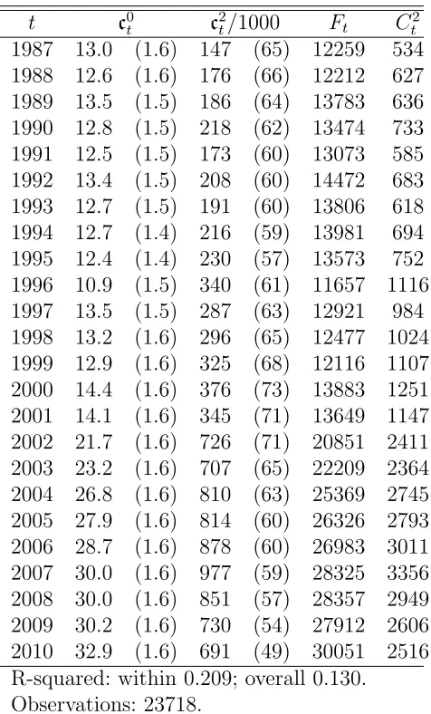
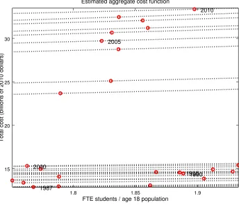
Table 2 presents the estimates. We found it necessary to impose c1_t = 0 to ensure an increasing aggregate cost function over the relevant range ofN. Figure3plots the aggregate cost function over time and circles the realized values from each year.

19_{We allow}_K _{to vary over time in the estimation (it is the number of colleges in the sample) but treat it} as fixed here to simplify the exposition.

20_{We assume that}∑

iαi = 0 and

∑

(23)

t c0_t c2_t/1000 Ft C_t2

1987 13.0 (1.6) 147 (65) 12259 534

1988 12.6 (1.6) 176 (66) 12212 627

1989 13.5 (1.5) 186 (64) 13783 636

1990 12.8 (1.5) 218 (62) 13474 733

1991 12.5 (1.5) 173 (60) 13073 585

1992 13.4 (1.5) 208 (60) 14472 683

1993 12.7 (1.5) 191 (60) 13806 618

1994 12.7 (1.4) 216 (59) 13981 694

1995 12.4 (1.4) 230 (57) 13573 752

1996 10.9 (1.5) 340 (61) 11657 1116

1997 13.5 (1.5) 287 (63) 12921 984

1998 13.2 (1.6) 296 (65) 12477 1024

1999 12.9 (1.6) 325 (68) 12116 1107

2000 14.4 (1.6) 376 (73) 13883 1251

2001 14.1 (1.6) 345 (71) 13649 1147

2002 21.7 (1.6) 726 (71) 20851 2411

2003 23.2 (1.6) 707 (65) 22209 2364

2004 26.8 (1.6) 810 (63) 25369 2745

2005 27.9 (1.6) 814 (60) 26326 2793

2006 28.7 (1.6) 878 (60) 26983 3011

2007 30.0 (1.6) 977 (59) 28325 3356

2008 30.0 (1.6) 851 (57) 28357 2949

2009 30.2 (1.6) 730 (54) 27912 2606

2010 32.9 (1.6) 691 (49) 30051 2516

R-squared: within 0.209; overall 0.130. Observations: 23718.

Note: standard errors are in parentheses; millions of 2010 dollars.

(24)

1.8 1.85 1.9 15

20 25 30

FTE students / age 18 population

Total cost (billions of 2010 dollars)

Estimated aggregate cost function

1987

1990 1995 2000

2005

2010

(25)

3.4

Joint Calibration

We determine the remaining parameters (ν, ξ, γ, χθ, χq, ζF, α) jointly such that the initial

steady state matches the following moments in 1987: average earnings, average net tuition,

the two-year cohort default rate, the correlation between parental income and enrollment,

the enrollment rate, the average grant size, and the percent of students with loans.21

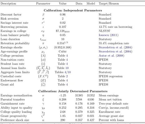
Table 3summarizes the calibration. Note that, while the table associates each parameter in the joint calibration with an individual moment, the calibration identifies the parameters

simultaneously, rather than separately. We discuss model fit in the next section.

Table 3: Model Calibration

Description Parameter Value Data Model Target/Reason

Calibration: Independent Parameters

Discount factor β 0.96 Standard

Risk aversion σ 2 Standard

Savings interest rate r∗ 0.02 Standard

Borrowing premium ι 0.107 12.7% rate on borrowing

Earnings in college eY $7,1282010 NLSY97

Loan balance penalty η 0.05 Ionescu(2011)

Loan duration tmax 10 Statutory

Retention probability π 0.5541/5 55.4% completion rate

Earnings shocks (ρ, σz) (0.952,0.168) Storesletten et al.(2004)

Age-earnings profile µj Cubic Storesletten et al.(2004)

College premium {λ} Table4 Autor et al.(2008)

Non-tuition costs {ϕ} Table4 IPEDS

Student loan rate {i} Table4 Statutory

Annual loan limits {bs_j, bu_j, bj} Table10 Statutory

Aggregate loan limits {ls, lu, l} Tables4/10 Statutory

Custodial costs {F, C2_} _Table₂ _{IPEDS regression}

Endowment flow {E} Table4 IPEDS

Grant aid {ζ} Table4 IPEDS

Calibration: Jointly Determined Parameters

Earnings normalization ν -1.25 31385 31352 Mean earnings

Parental transfers ξ 0.208 5788 6100 Mean net tuition

Garnishment rate γ 0.158 0.176 0.169 Two-year default rate

Ability input to quality χθ 0.252 0.295 0.316 Corr(p. income,enroll)

College quality loading χq 2.68 0.379 0.325 Enrollment rate

Grant progressivity ζF _1.85 _0.027 _0.021 _{Average grant size}

Preference shock size α 290 0.357 0.427 Percent with loans

Note:{x} meansxhas a transition path given in Table4; $xyyyy means $x, measured nominally inyyyy dollars, converted to model units.

(26)

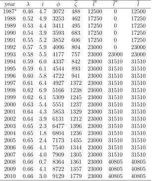
year λ i ϕ ζ ls lu l

1987∗ 0.46 4.7 3072 488 12500 0 12500

1988 0.52 4.9 3253 462 17250 0 17250

1989 0.53 4.4 3411 495 17250 0 17250

1990 0.54 3.9 3593 683 17250 0 17250

1991 0.55 5.2 3852 606 17250 0 17250

1992 0.57 5.9 4006 804 23000 0 23000

1993 0.58 5.5 4177 757 23000 23000 23000

1994 0.59 6.0 4337 842 23000 31510 31510

1995 0.59 6.1 4544 893 23000 31510 31510

1996 0.60 5.8 4722 941 23000 31510 31510

1997 0.61 6.4 4927 1372 23000 31510 31510

1998 0.62 6.9 5166 1238 23000 31510 31510

1999 0.62 6.1 5309 1245 23000 31510 31510

2000 0.63 5.4 5551 1237 23000 31510 31510

2001 0.64 4.3 5853 1329 23000 31510 31510

2002 0.64 3.9 6131 1212 23000 31510 31510

2003 0.65 2.3 6477 1396 23000 31510 31510

2004 0.65 1.8 6804 1236 23000 31510 31510

2005 0.65 2.4 7173 1455 23000 31510 31510

2006 0.66 4.1 7540 1344 23000 31510 31510

2007 0.66 4.0 7909 1305 23000 31510 31510

2008 0.66 0.7 8364 1361 23000 40805 40805

2009 0.66 4.1 8722 1357 23000 40805 40805

2010 0.66 3.0 9129 1779 23000 40805 40805

Note: Except for ζ, all dollar values are nominal but con-verted to real in the computation.a_{The “1987” borrowing} limits correspond to the limits in place from 1981 to 1986. The “1987” college premium corresponds to the average from 1981 to 1987.b_{The interest rates here correspond to} five-year averages. See AppendixB for details. The nota-tion lu (lu = 0 prior to 1993 and then lu = l afterward) represents the aggregate unsubsidized loan limit.

(27)

3.5

Model Fit

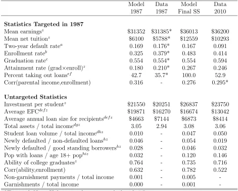
Table5presents key higher education statistics from the model and the data. The calibration

of the initial steady state directly targets the first set of statistics from 1987, while the

remaining statistics act as an informal test of the model. Note that, while the calibration

matches mean earnings, net tuition, and the two-year default rate from 1987 quite well, the

model generates too little enrollment and too many students with loans.

We pinpoint two sources for these shortcomings. First, the presence of only one college in

the model generates too much market power, which results in a small calibrated value for the

parental transfers parameterξin order to still match average net tuition. Thus, students rely

more on borrowing. Second, by omitting ability terms in the post-college earnings process,

we implicitly attribute the entire college premium to the sheepskin eﬀect of a diploma (as

opposed to selection eﬀects). This exaggerated sheepskin eﬀect generates a larger surplus

from attending college, which the college partially captures through higher tuition.

Despite the presence of too many student borrowers, the model actually generates smaller

average loans than in the data—$4,700 vs. $7,100. Lastly, the model nearly matches invest-ment per student of $20,300 in 1987 and the ratio of assets to income of about 3. The

matching of the asset-to-income ratio reflects the fact that our model of households is, at its

core, a standard incomplete markets life-cycle model.

4

Results

Now we present the main results. First, we compare the model’s initial and terminal steady

states to the data from 1987 and 2010. Next, we evaluate the transition path of the model in light of the time series data. Lastly, we undertake a number of counterfactual experiments

to quantify the explanatory power of each theory about the rise in college tuition.

4.1

Steady State Comparisons

4.1.1 Tuition

Of central importance, the model generates a 106% increase in average net tuition—from

approximately $6,100 to $12,600—between the initial and terminal steady states. This jump

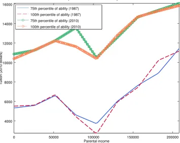
compares to a 78% increase in the data. To illustrate how tuition changes, figure 4 plots slices of the tuition function and figure 12in appendix Cplots the entire function.

In both steady states, tuition does not move monotonically with income. Instead, tuition

(28)

0 50000 100000 150000 200000 4000

6000 8000 10000 12000 14000 16000

Parental income

Tuition (2010 dollars)

Equilibrium tuition for select ability levels 75th percentile of ability (1987)

100th percentile of ability (1987) 75th percentile of ability (2010) 100th percentile of ability (2010)

(29)

Model Data Model Data

1987 1987 Final SS 2010

Statistics Targeted in 1987

Mean earningsz _$31352 _$31385* _$36013 _$36200

Mean net tuitionz _$6100 _$5788* _$12559 _$10293

Two-year default ratea 0.169 0.176* 0.167 0.091

Enrollment rateb _0.325 _0.379* _0.483 _0.414

Graduation ratec _0.554 _0.554* _0.554 _0.594

Attainment rate (grad×enroll)z 0.180 0.210* 0.267 0.246

Percent taking out loansef _42.7 _35.7* _100.0 _52.9

Corr(parental income,enrollment) 0.316 - 0.276 0.295*

Untargeted Statistics

Investment per studentz _$21550 _$20251 _$26837 _$23750

Average EFCdef z $19871 $16270 $16674 $13042

Average annual loan size for recipientsdef z _$4663 _$7144 _$6873 _$8414

Total assets / total incomedgz _3.05 _2.94 _3.08 _3.06

Student loan volume / total incomedhz 0.010 - 0.047 0.050

Newly defaulted / non-defaulted loanshz _0.046 _- _0.054 _0.019

Newly defaulted / good standing borrowershz _0.028 _- _0.046 _0.032

Pop with loans / age 18+ pophiz 0.032 - 0.120 0.146

Ability of college graduatesz _0.764 _- _0.735 _0.716

Corr(ability,enrollment) 0.632 - 0.782 0.522

Non-garnishment payments / total income 0.001 - 0.005

-Garnishments / total income 0.000 - 0.001

-*Targeted. Note: Unknown values are marked with “-”.

Sources: a_stu ₍₂₀₁₅_); b_nce ₍_2015a_); c_nce ₍_2015b_); d_FRE_; e_{Tables 2 and 7 in} _{Wei et al.} (2004); fTables 2.1-C and 3.3 Bersudskaya and Wei (2011); gBEA; hfed; iHowden and Meyer (2011); and z_{authors’ calculations.}

(30)

income levels between $50,000 and $100,000 as financial aid eligibility tightens and grants

decline. After $100,000, tuition resumes its ascent as student ability to pay increases. The

tuition curves shift up noticeably between the two steady states, though not in a parallel

fashion. In particular, the region of declining tuition compresses to the range between $75,000

and $100,000, which is largely due to the expansion in aid between 1987 and 2010.

Comparatively, the college engages in more modest price discrimination by academic

ability than by parental income.22 Inspection of the 100th percentile and 75th curves in

1987 reveals that tuition never diﬀers by more than $700 between moderate and high ability

students. By 2000, the largest tuition diﬀerence between the 75th and 100th percentiles of

the ability distribution rises to $2,000.

When weighing whether to oﬀer tuition discounts to high ability students, colleges face

the trade-oﬀ between a higher ability student body and the need for resources to fund

quality-enhancing investment expenditures. In our calibration, the latter eﬀect dominates. The data

provides supporting evidence. For instance, table5, which presents selected statistics from the

data and the initial and terminal steady states, shows that investment in the model increases

by 25% between the two steady states. This increase approximates well the untargeted 17%

rise in the data. While we lack data on student ability in 1987, the model’s mean college

graduate ability of 0.735 in 2010 closely matches the untargeted 0.716 from the data.

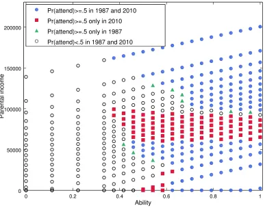
4.1.2 Enrollment

Figure5 reveals how the enrollment patterns change between the steady states. Recall that

the calibration targets the correlation between parental income and enrollment, and observe

that average student ability aligns closely with the data in table5. However, figure5unveils a

striking polarization of enrollment by income in the initial steady state. Specifically,

middle-income students find themselves priced out of college, enrolling at a rate of less than 50%.

As shown in equation 14, colleges set tuition by charging each student their type-specific eﬀective marginal cost EM C(sY) plus a markup that reflects the student’s willingness to

pay. Given that eﬀective marginal cost only depends on the ability component x(sY) of

each student’s type, all tuition variation within ability types derives from the impact of

parental income and access to financial aid on student willingness to pay.23 _Furthermore,

in the absence of preference shocks (the limiting case as α → ∞), colleges first only admit

22_{In fact, theoretically, tuition should be monotonically decreasing in ability. However, due to} computa-tional cost, we have parametrized the tuition function more flexibly in the income dimension to account for more variation there. See appendixCfor computation details.

23_{Replicated here:}_T₍_s

Y) + P

(enroll|sY;T(·), q)

∂P(enroll|sY;T(·), q)/∂T

| {z }

(∂logP/∂T)−1

=C′(N) +I+qθ

qI (θ−x)

| {z }

(31)

0 0.2 0.4 0.6 0.8 1 0

50000 100000 150000 200000