Issues
ISSN: 2146-4138
available at http: www.econjournals.com
International Journal of Economics and Financial Issues, 2019, 9(4), 228-240.
Inward Foreign Direct Investment and Welfare Nexus: The
Impact of Foreign Direct Investment on Welfare in Developing
Countries
Md. Shakib Hossain
1, Md. Shahin Kamal
2, Md. Rubaeth Halim
3, Nurul Mohammad Zayed
4*
1Department of Business Administration, East West University, Dhaka, Bangladesh, 2 Senior Principal Officer,
Arab Bangladesh Bank, Bangladesh,3Finance and Controlling Specialist, DHL Global Forwarding (Bangladesh) Ltd., Dhaka, Bangladesh, 4Department of Real Estate, Faculty of Business and Entrepreneurship, Daffodil International University, Dhaka, Bangladesh. *Email: zayed.bba@daffodilvarsity.edu.bd
Received: 25 May 2019 Accepted: 22 July 2019 DOI: https://doi.org/10.32479/ijefi.8465
ABSTRACT
It is an attempt to estimate the consequence on welfare because of foreign direct investment (FDI) in different developing countries, mainly incorporated
with the panel data having 79 countries producing over 1,343 observations from 1998 to 2014. Panel unit root test, panel cointegration, vector error correction model (VECM), panel dynamic least squares, fully modified least square method, fixed effect model and random effect model have used
for determining the consequence on welfare due to FDI. According to the VECM, it interprets that there is a long run causality of the variables such
as FDI, agglomeration, debt, governance, inflation, infrastructure, openness, bureaucracy and country risk with the welfare. Concentrating on panel dynamic least squares and fully modified least square method that interprets if the FDI goes up by 1 unit the welfare goes up 0.286751 and 0.227956 respectively and from the both fixed effect model and random effect model elucidate that FDI is a significant variable to explain the welfare.
Keywords: Panel Unit Root Test, Panel Cointegration, Vector Error Correction Model, Foreign Direct Investment JEL Classifications: C23, F21, I3
1. INTRODUCTION
Foreign direct investment (FDI) promotes the continuous economic and social development by transferring technology, skill development, innovation and management efficiency both developed and developing country. This study is mainly accentuated on determining the host countries’ overall welfare
gain due to the incessant flow of FDI. Li and Liu (2005) examine a panel of 84 countries over the period 1970-1999 to understand
whether FDI triggers economic growth. Their result reveals that FDI not only promotes growth directly, but also increase growth with its interaction term. They further test their hypothesis in two sub-sample; developed and developing countries by dividing the whole sample (84 countries). Again the result confirms
that in both developed and developing countries FDI promotes
economic growth. They find that a 10 percent increase in FDI (as
a percentage of GDP) leads to a 4.1 percentage-point increase in the rate of economic growth. Due to FDI, generates massive and radical transition in socio-economic phenomenon in host countries especially in stronger welfare functions such as increased
education and life expectancy, in addition to the increased
purchasing power and spillover effects.
Hansen and Rand (2006) search for co-integration and causality
relation between FDI and growth in a sample of 31 developing
countries for the period 1970-2000 and they confirm the existence of co-integration. Moreover, their result indicates that
FDI has a lasting positive impact on GDP irrespective of level
of development. They interpret their findings “as the evidence
in favor of the hypothesis that FDI has an impact on GDP via knowledge transfer and adoption of new technology”. With the
substantial flow of FDI assists to upgrade and accelerate the efficiency level of the labor forces in developing country through
schooling, training and compelling layoffs. FDI leads human capital formation through upgrading the skills of human capital of host countries by provision off formal training, schooling and spill-over effects of layoffs and turnover of labor force from
international firm to domestic firms. On the demand side, FDI
may positively affect the accumulation of human capital. These are technology transfer, spillovers, and physical capital investment. On the supply side the process is less well known and documented, but FDI can affect human capital development via its effect on
general education, and official and informal on-the-job training.
When the FDI has increased that will increased the employment
opportunities, when the employment opportunities is flourishing that reflects increasing the household purchasing power and ultimately that makes consequence significantly on the social
welfare (health, standard of living).
Acceleration of FDI makes consequence on infrastructure and other macroeconomic factors. There are a diverse opinion regarding the welfare and FDI. According to the Arcelus et al.
(2005); Anand and Sen (2000); Meyer (2004); Meyer and Sinani (2009); Globerman and Shapiro (2003); Rogers (2004), FDI makes a significant effect on welfare and on the other hand according to the Konings (2001); FDI does not effect on the welfare. This article
shows empirically that FDI offers a development potential and contributes to the host country’s welfare. This article is organized
as the following segment literature review, model specification,
results and analysis and conclusion.
2. LITERATURE REVIEW
Because of FDI, whether the welfare gain in terms of technology, knowledge, absorbing capacity, management efficiency, infrastructure and manifold social issue for the host countries is conceptually and virtually argumentative issue. Welfare cannot
measuring on a conclusive and specific terms. Overall welfare
may incorporate with the macroeconomic effects, social issues, and the natural environment. Economic welfare that is usually measured in terms of GDP or other measures such as income and purchasing power, in order to determine functions of utility and
efficiency (e.g., Kakwani, 1981; McKenzie and Pearce, 1982). Overall measures of welfare expand on this economic base,
highlighting other indicators of prosperity and quality of living
(Pyatt, 1987), the most prevalent of these being the United Nations’ human development index (Anand and Sen, 2000).
On the concentration of Anand and Sen (2000) elucidation that
the overall welfare as encompassing the three components of the
human development index (HDI: Life expectancy, education,
GDP), as well as a measure of country infrastructure such as its
capacity to utilize knowledge from the firm (e.g., Blomstrom and Kokko, 2003; Chen, 1996; Rogers, 2004).
Current literature has been divided by the both positive and negative impacts of FDI on the host country. According to Arcelus
et al. (2005) studied the effects of foreign capital flows on each of the three dimensions of the UN’s human development index (HDI). They argue that those countries that are more efficient
in their utilization of FDI have greater control on their welfare development. Though, this work did not take into account the
role of knowledge and government structure that also influence
overall welfare.
FDI that makes an affects on the natural environment, social issues, such as health care, government and educational institutions, and
local economies (e.g., Anand and Sen, 2000), which are the primary
importance factors for the recipient economies. FDI has a strong
positive effect on the host country (e.g., Bain, 1951; Buckley, 1990; Hymer, 1968; Penrose, 1956), and the inflow of funds provides
additional resources to the market economy (e.g., Mirza and
Giroud, 2004). FDI stimulate more capital-intensive investment in host countries and a better-developed domestic financial market
is more effective in promoting economic growth.
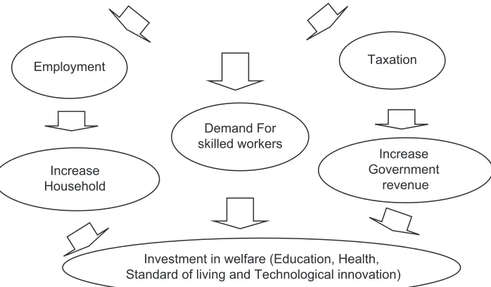
Figure 1 highlights FDI’s contributions to the host country’s welfare via three channels: The labor market, households, and government. FDI would contribute to welfare by increasing
government revenue through taxation by which they can further
develop and maintain social welfare such as increasing literacy,
health care, and employment benefits; through increased household
income and purchasing power; and by driving the need for skilled
workforce (MacDougall, 1960). Both host-country governments and households are able to use a portion of the extra income
to invest in welfare (i.e., improved education, health, standard of living, technological innovation, and infra- structure).
However, the efficiency of such allocation will depend on the
absorptive capacity of the host country and quality of governance
(e.g., Globerman and Shapiro, 2003; Rogers, 2004).
FDI facilitated manifold employment creation especially with
the Greenfield investment and created employment generation
with the forward and backward linkage with the many domestic
firms. Because of FDI, the purchasing power of the host countries
citizen is augmented.
According to Chakrabarti (2001); Asiedu (2002) and Zhao (2003)
pointed out that higher economic growth results in greater FDI
inflows as it is a measure of the attractiveness of the host countries. Lucas (1993) and Cernat and Vranceanu (2002) argued that as economic growth rises, FDI inflows into host countries tend to
be encouraged.
FDI also makes a positive effect on education. Borensztein et al. (1998) conclude that FDI is a vehicle for the adoption of new technology, and therefore, the training required to prepare the labor force to work with new technologies suggest that there may also be an effect of FDI on human capital accumulation. The relation between the FDI and human capital is highly linear and multiple equilibrium. Host country with having the accumulation
of ambidextrous skill labor forces magnetizes a vast amount of
of a country along with the enhancing the adaptability and capabilities of the workforces. When an individual incomes propagate due to the FDI that effects on the health security, carefully organize and maintain his subsistent needs.
Direct investment on the concentration of infrastructure ensures
efficient production facilities and stimulates economic activities,
alleviate transaction cost and trade costs improving competitiveness and ensure ample employment opportunities for the poor. FDI and infrastructure has a positive relationship. Different studies on
developing countries (e.g., Mengistu and Adams, 2007); emerging economies (e.g., Zhang, 2001); Western Balkan Countries (e.g., Kersan-Skabic and Orlic, 2007) and Southeast European Countries (e.g., Botric and Skuflic, 2006) show the significant role of infrastructure development in attracting the inflow of FDI.
When FDI has increased, over time there will also be an increase
in overall welfare as reflected by institutional and macroeconomic effects, social welfare, the natural environment, and local firms (e.g., Anand and Sen, 2000).
The empirical evidence on FDI and economic growth is ambiguous, although in theory FDI is believed to have several positive effects on the economy of the host country (such as productivity gains, technology transfers, the introduction of new processes, managerial skills and know-how, employee training)
and in general it is a significant factor in modernizing the host
country’s economy and promoting its growth. Considerable
empirical evidence illustrates that FDI not to be beneficial for
economic growth and development in host countries.
FDI creates miserable income inequality gaps rather resolving the problems due to the income inequality economic activities
is restraints and economic advancement is deteriorated. Driffield and Girma (2003) demonstrate that there are two distinct effects
that contribute to FDI increasing inequality. Firstly, there is the effect that stems from inward investment increasing the demand for skilled labour in the host location, such that the wages of such
workers are bid up. Secondly, Barrel and Pain (1996) demonstrate that inward investment replaces unskilled labour, again reducing
the returns to such workers. Barrell and Pain (1997) show inward
investment introduces new technology and generates a decline in the overall demand for unskilled labour.
There are mixed opinion about the welfare gain for host country
from the FDI. Concentrate on the research focus the work generally consider that FDI makes a spillover effects on social issue, health care, education attainment, employment generation and positive effect on individual purchasing power and indubitable propagate economic functions.
3. MODEL SPECIFICATION
This paper is mainly concentrate on determining the relationship with the FDI and the welfare. The paper has used different control
variables, debt, governance, inflation, infrastructure, openness,
agglomeration and country risk. As part of the methodological design, the basic equation is illustrated below:
Welfare = α0+α1FDI+α2Agglomeration+α3Debt+α4Goverance+
α5Inflation+α6Infrastructure+α7Openness+α8Bureaucracy
+α9Country Risk+et (1)
Where α0, α1-α9 are parameters to be estimated.
et is stochastic error terms assumed to be independently and identically distributed.
For estimating the relationship between welfare and FDI, here the paper is using different statistical methods like panel unit root test, panel co-integration, fully modified OLS and
dynamic OLS method and fixed effect and random effect
regression.
Taxation
Demand For skilled workers Increase
Household
Investment in welfare (Education, Health, Standard of living and Technological innovation) Employment
Increase Government
revenue
Figure 1: Foreign direct investmentinflow: The mechanism to human development
3.1. Panel Unit Root Test: Levin, Lin and Chu
Levin, Lin and Chu start panel unit root test by consider the
following basic ADF specification.
DY = Yit it 1+ itDYit j+ Xit* + it
j=1 Pi
α −
∑
β − δ ε (2)Where, DYit = difference term of Yit Yit1 = panel data
α = ρ–1
pi = the number of lag order for difference terms
X*it = exogenous variable in model such as country fixed effects and individual time trend
εit = the error term of equation 2.
LLC panel unit root test has null hypothesis as panel data has unit root as well as can present below that:
H0: Null hypothesis as panel data has unit root (assumes common unit root process)
H1: Panel data has not unit root.
3.2. Im, Pesaran and Shin Test
The properly standardized t*NT has an asymptotic standard normal distribution and also it was rewritten to be new t-statistics as well as can show below that: (see equation 3).
W n t N E t p
N var t p
t NT NT
1
iT i
1
ix i i
* = √ −
(
( )
)
/
√
(
( )
)
−
−
∑
t =1n
==
∑
1
n
(3)
Where, Wt*NT is W-statistics has been used to test panel data based on Im, Pesaran and Shin techniques. Also this technique has non-stationary as null hypothesis as well as to show below that: H0: Null hypothesis as panel data has unit root (assumes
individual unit root process) H1: Panel data has not unit root.
3.3. Fisher-type Test using ADF and PP-test (Maddala and Wu and Choi)
Madala and Wu proposed the use of the Fisher (Pλ) test which is
based on combining the P-values of the test-statistics for unit root in each cross-sectional unit. Let pi are U [0,1] and independent, and −2logepi has a χ2 distribution with 2N degree of freedom and can be written in equation 4.
P λ = −2
∑i=1
N log pe i (4) Where, Pλ = Fisher (Pλ) panel unit root testN = all N cross-section
−2
∑
log pe i i=1 N= it has a χ2 distribution with 2N degree of freedom.
In addition, Choi demonstrates that in equation 5.
Z 1 Ni 1 i1 p N 1
i 1 i
=
(
√)
( )
− − >
( )
=
∑
= −/ N ¸ 0, (5)
Where, Z = Z-statistic panel data unit root test
N = all N cross-section in panel data
θi 1
− = the inverse of the standard normal cumulative distribution function
pi = it is the P-value from the ith test.
Both Fisher (P) Chi-square panel unit root test and Choi Z-statistics
panel data unit root test have non-stationary as null hypothesis as well as to show below that:
H0: Null hypothesis as panel data has unit root (assumes individual unit root process)
H1: Panel data has not unit root.
3.4. Hadri Test
The Hadri test for panel data has the hypothesis to be tested is H0 is null hypothesis and H1 is against null hypothesis and can show below that:
H0: Null hypothesis as panel data has not unit root (assumes common unit root process)
H1: Panel data has unit root.
Five different panel unit test is being accomplished (Levin, Lin and Chu, Im, Pesaran and Shin, Fisher-type test using ADF and PP-test (Maddala and Wu and Choi) and Hadri for measuring that the data are stationary or not.
3.5. Panel Cointegration Test
In order to solve the spurious regression problem and violation of the assumptions of the classical regression model, co-integration
analysis is used to examine the long run relationship between the
variables. This test is mainly accomplished for identifying the long run relationship between welfare and FDI.
The starting point of the residual-based panel co-integration test statistics of Pedroni is the computation of the residuals of the hypothesized co-integrating regression.
Yi,t = α1+β1ix1i,t+β2ix2 i,t+…+βMixM i,t+ei,t,t=1,…T;i=1,…N (6)
Here, Y indicates the dependent variable like welfare and X1 to Xm indicates the different independent variables (see in details Table 1).
Another method have used that is known as a Kao for estimating the long run relationship between the variables.
Kao uses both DF and ADF to test for co-integration in panel as well as this test similar to the standard approach adopted in the EG-step procedures. Also this test start with the panel regression
model as set out in equation 7.
Yit = Xitβit+Zitγ0+εit (7)
Where Y and X are presumed to be non-stationary and (see equation 8):
e = e + Vit ρ it it (8)
amounts to test H0: ρ = 1 in equation 21I against the alternative
that Y and X are co-integrated (i.e., H1: ρ < 1).
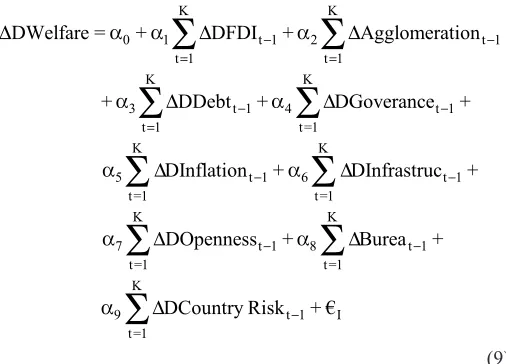
3.6. Vector Error Correction Model (VECM)
The purpose of VECM model is to indicate the speed of adjustment from the short run equilibrium to the long run equilibrium state between the variables from welfare to country risk. The greater
the coefficient of the parameter the higher the speed of adjustment
of the model from short runs to long run. Considering the basic
equation (1), the VECM model is specified as follows:
K K
0 1 t 1 2 t 1
t 1 t 1
K K
3 t 1 4 t 1
t 1 t=1
K K
5 t 1 6 t 1
t=1 t=1
K K
7 t 1 8 t 1
t=1 t=1
K 9
t=1
DWelfare = + DFDI + Agglomeration
+ DDebt + DGoverance +
DInflation + DInfrastruc +
DOpenness + Burea +
DCountry R
− −
= =
− −
=
− −
− −
∆ α α ∆ α ∆
α ∆ α ∆
α ∆ α ∆
α ∆ α ∆
α ∆
∑
∑
∑
∑
∑
∑
∑
∑
∑
isk + €t 1− I(9) Where the €I is the error term, ECM (−1) is the error correction term, βicaptures the long run impact. The short run effects are
captured through the individual coefficients of the differenced
terms (α) while the coefficient of the ECM variable contains
information about whether the past values of variables affect
the current values. The size and statistical significance of the coefficient of the ECM measures the tendency of each variable to return to the equilibrium. A significant coefficient implies that
past equilibrium errors play a role in determining the current outcomes.
3.7. Fully Modified OLS and Dynamic OLS Method
A standard panel OLS estimator for the coefficient βi given by:
βi t =1 it i* 2 T
i=1
N 1
i=1 N
it i *
it i * t =1
T
, OLS =[ (X X ) ]
(X X )(Y Y )
−
− −
∑
∑
−∑
∑
∑
(10)Where, i = cross-section data and N is the number of cross-section t = time series data and T is the number of time series data
βi,OLS = a standard panel OLS estimator Xit = exogenous variable in model
X*i = average of Xi*
Yit = endogenous variable in model Yi* = average of Yi*.
FMOLS estimator that incorporates the Phillips and Hansen
(1990) semi-parametric correction to the OLS estimator to
adjusts for the heterogeneity that is present in the dynamics underlying X and Y. Specifically, the FMOLS statistics is: (see equation 11).
Table 1: Description of the variables
Variable Description Source Expected
sign Dependent
variable Welfare Life expectancy Health dimension is assessed by life expectancy at birth HDI, 2014 (+)
Education attainment The education dimension is measured by
mean of years of schooling for adults aged
25 years and more and expected years of
schooling for children of school entering age
GDP per capita (PPP
US$) The standard of living dimension is measured by gross national income per
capita Independent
variable FDI inflow Total FDI inflows a host country receives at time t divided by the host country’s total population (i.e., FDI per capita) UNCTAD, 2014 (+)
Control
variable Agglomeration Assesses the prevalence of foreign firms in the country. Based on the item: “Foreign ownership of companies in your country is (1=rare and
limited, 7=prevalent and encouraged.”
Global competitiveness
report, 2014
Debt Total debt/GDP WDI, 2014 (−)
Governance Governance includes voice and accountability, political stability and
violence, government effectiveness, regulation quality, rules of law, control of corruption
Worldwide governance
indicators, 2014 (+)
Inflation Inflation as measured by the consumer price index which measures
annual % change in a fixed basket of goods WDI, 2014 (−)
Infrastructure Telephone mainlines per 1000 people for entire country WDI, 2014 (+)
Trade
openness Trade is the sum of exports and imports of goods and services measured as a share of gross domestic product WDI, 2014 (+)
Bureaucracy Number of days to start a business. Global competitiveness
report, 2014 (−)
Country risk Terror scale: 1 (very safe) and 5 (very risky) Global competitiveness
βi 1
it i* 2 t =1
T i=1
N 1
it i * t =1
T
it
, FMOLS = N (X X ) ]
(X X )(Y TY
− −
+
−
− −
∑
∑
∑
[
ii) (11)
Where, i = cross-section data and N is number of cross-section data t = time series data and T is number of time series data
βi,FMOLS = full modified OLS estimator
Xit = exogenous variable in model
X*i = average of Xi*
Yit = endogenous variable in model Yi* = average of Yi*
Yit+= Xα it−X*i)−
(
Ω21i/Ω22i)
∆Xit and Ω is covariance. In contrast to the non-parametric FMOLS estimator, Pedroni has also constructed a between-dimension, group-means panel DOLS estimator that incorporate corrections for endogeneity and serial correlation parametrically.βi 1 t =1 it i* T i=1 N
it it t =1 T
, DOLS= N− Z Z ) Z Z
−
∑
∑
∑
[ ( )]
1
(12)
Where, i = cross-section data and N is number of cross-section data t = time series data and T is number of time series data
βi,DOLS = dynamics OLS estimator
Zit = is the 2(K+1)×1
Zit = (Xit–X*i) X*i = average of Xi*
∆Xi,t–k = differential term of X.
3.8. Fixed Effect and Random Effect Regression
Fixed and random effect regression model is used to see that whether the FDI is a significant element to explain the
welfare.
Here the fixed effects regression model is
Yit = β0+β1X1,it+…+βKXk,it+γ2E2+…+γnEn+δ2T2+…+δtTt+ui (13)
Where, Yit = is the dependent variable (DV) (welfare) where i = entity and t = time
Xk,it = represents independent variables (FDI, agglomeration, debt,
governance, inflation, infrastructure, openness, bureaucracy,
country risk
βk = is the coefficient
uit = is the error term En = is the entity n
γ2 = is the coefficient for the binary regressors (entities)
Tt = is time as binary variable (dummy), so we have t–1 time
periods
δt = is the coefficient for the binary time regressors.
The random effects model is:
4Yit = βXit+α+uit+εit (14)
3.9. Data Sources
This article has employs panel data for 79 countries over the period from 1998 to 2014 among different developing countries
(Table 2). For the dependent variable (Welfare), the data that
have used from the UN Development Program, 2014. The FDI
which is noted as an independent variable is measured in current U.S. dollars divided by the host country’s total population as the dependent variable, and data come from UNCTAD. Data on FDI are provided by several sources, such as Balance of Payments Statistics Yearbook and International Finance Statistics by the international monetary fund (IMF), European Union Direct Investment Yearbook by EUROSTAT, World Investment Report by UNCTAD, World Development Indicators by the World Bank, and International Direct Investment Statistics Yearbook by OECD. Only the UNCTAD, OECD, and EUROSTAT offer
a sectoral breakdown of FDI flows and stocks. The drawback is
that OECD and EUROSTAT only cover a very limited number of world countries and thus the total direct investment received by any given country cannot be completely assessed. Moreover,
the paper is more interested in FDI inflows than FDI stocks
because policy recommendations are usually formulated to
boost FDI inflows rather than to accumulate FDI stocks for a
given period. However, only UNCTAD provides a break down into two different categories: FDI figures for developed and for developing countries that really serve our purpose. Because of making contemplative judgment FDI related data from accumulated from the UNCTAD.
For accomplishing the research purpose for different control variables data are accumulated from the manifold sources, the
data on the degree of openness, the inflation rate, debt and the
infrastructure come from the World Bank’s World Development Indicators (Table 2). Governance variable that including the six
different factors, voice and accountability, political stability and violence, government effectiveness, regulation quality, rules of law and control of corruption. Data are aggregating from the worldwide governance indicators. Data collection method and research methodology all the things can be access in that particular website: www.govindicators.org. For another control variable, like agglomeration the data that have used from the global
competitiveness report, the index value from 1 to 7, 1 represent rare and 7 represent prevalent. Country risk relevant data are aggregating from the global competitiveness report, 2014 which terror scale 1
(very safe) and 5 (very risky). For Bureaucracy related data are also
aggregating from the global competitiveness report, 2014.
Table 2: List of the countries
Afghanistan, Albania, Algeria, Angola, Argentina, Armenia, Azerbaijan, Bangladesh, Belarus, Benin, Bhutan, Bolivia, Botswana, Bulgaria, Burundi, Cambodia, Chad, Colombia, Comoros, Cuba, Dominica, Ecuador, El Salvador, Ethiopia, Figgie, Gambia, Georgia, Ghana, Grenada, Guatemala, Guinea, Guyana, Haiti, Honduras, Iran, Iraq, Jamaica, Jordan, Kazakhstan, Kenya, Kosovo, Lebanon, Liberia, Libya, Madagascar, Maldives, Mali, Moldova, Mongolia, Morocco, Mozambique, Myanmar, Namibia, Nepal, Nicaragua, Nigeria, Pakistan, Papua New Guinea, Peru, Senegal, Serbia, Sierra Leone, Somalia, South Sudan, Sri Lanka, Sudan, Suriname, Tajikistan, Timor-Leste, Togo, Tonga, Tunisia, Uganda, Ukraine,
4. RESULT AND ANALYSIS
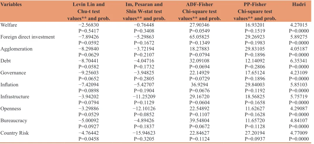
Concentrate on the model specification the following Table 3 interprets whether the panel data are stationary or not. For
identifying this, five different panel unit test is being accomplished
(Levin, Lin and Chu, Im, Pesaran and Shin, Fisher-type test using ADF and PP-test (Maddala and Wu and Choi) and Hadri.
Base on the five different type of panel unit root test such as
Levin, Lin and Chu, Im, Pesaran and Shin, Fisher-type test using ADF and PP-test (Maddala and Wu and Choi) and Hadri method
the variables are not stationary at a level. Now let’s see at first difference the data are stationary or not. Here again using the five
different methods for identifying the data are stationary or not at
first differences. The following table illustrate that according to the Levin, Lin and Chu, Im, Pesaran and Shin, Fisher-Type test using ADF and PP-test (Maddala and Wu and Choi) and Hadri
methods the variables are stationary or not at first differences.
From the Table 3 concentrate on the five different type of panel
unit root test such as Levin, Lin and Chu, Im, Pesaran and Shin, Fisher-type test using ADF and PP-test (Maddala and Wu and
Choi) and Hadri methods the variables are stationary at a first
differences.
To solve the spurious regression problem and violation of the assumptions of the classical regression model, co-integration analysis
is used to examine the long run relationship between the variables.
From the no deterministic trends there are 7 different and separate
outcomes (Table 4). Out of 7 outcomes, 3 outcomes interpret that
accept the null hypothesis (H0 = no co-integration), because the P > 5. On the other hand 4 outcomes illustrates that reject the null hypothesis and accept the alternative hypothesis. Therefore it is to be noted that base on the no deterministic trend elucidate that the variables are co-integrate. On the other hand from the deterministic
intercept and trends way out of 7 outcomes 5 outcomes interpret
that accept the null hypothesis (H0 = no co-integration), because
Table 3: Panel unit root test
Variables Levin Lin and
Chu-t test values** and prob.
Im, Pesaran and Shin W-stat test values** and prob.
ADF-Fisher Chi-square test values** and prob.
PP-Fisher Chi-square test values** and prob.
Hadri
Welfare −2.56830
P=0.5417 −0.76448P=0.3408 P=0.054927.90346 16.93201P=0.1519 P=0.00004.27015
Foreign direct investment −7.89426
P=0.0592 −5.29863P=0.1672 P=0.134965.05825 29.26923P=0.1983 P=0.00005.89275
Agglomeration −8.29840
P=0.0629 −3.72194P=0.2107 P=0.079418.27883 29.83105P=0.1896 P=0.00004.05187
Debt −8.70441
P=0.0582 −4.04716P=0.1732 P=0.069432.09108 12.14092P=0.2806 P=0.00006.35341
Governance −9.25603
P=0.0652 −3.94825P=0.2805 P=0.072922.14929 17.65124P=0.1896 P=0.00004.23109
Inflation −7.42094
P=0.0898 −5.42707P=0.1904 P=0.067636.9294 29.84003P=0.1192 P=0.00005.85103
Infrastructure −3.94202
P=0.0794 −11.25209P=0.1129 P=0.060429.16720 18.56825P=0.1658 P=0.00005.75719
Openness −3.29886
P=0.0529 −12.10126P=0.0852 22.54892P=0.1107 P=0.162811.62627 P=0.00004.29087
Bureaucracy −5.00092
P=0.0927 −4.89426P=0.1837 P=0.067239.54804 P=0.112811.65720 P=0.00004.84107
Country Risk −4.76442
P=0.0458 −15.94623P=0.3205 22.84627P=0.1124 27.20194P=0.0937 P=0.00004.77009
Table 4: Pedroni residual co-integration test
Test method Pedroni residual co-integration test
No deterministic trend Deterministic intercept and trend No deterministic intercept or trend
Panel v-statistic −0.051728
P=0.6523 P=0.82560.8256 −0.743317P=0.4529
Panel rho-statistic −1.290032
P=0.3518 P=0.29540.2954 −0.852204P=0.1824
Panel PP-statistic −2.632710
P=0.0026 P=0.17620.1762 −1.430953P=0.0026
Panel ADF-statistic −2.861629
P=0.0014 P=0.43690.4369 −1.679403P=0.0054
Group rho-statistic 0.853944
P=0.6518 P=0.83110.8311 P=0.43261.243960
Group PP-statistic −3.167729
P=0.0006 P=0.00060.0006 −2.620219P=0.0002
Group ADF-statistic −4.258803
the P > 5. On the other hand 2 outcomes illustrates that reject the null hypothesis, it means that accept the alternative hypothesis. Therefore it is to be noted that base on the deterministic intercept and trend elucidate that the variables are not co-integrate. From
the no deterministic intercept and trends out of 7 outcomes
4 outcomes interpret that reject the null hypothesis (H0 = no
integration), because the P < 5. On the other hand 3 outcomes
illustrates that accept the null hypothesis, it means that reject the alternative hypothesis Therefore it is to be noted that base on the no deterministic intercept and trend method elucidate that the variables are co-integrated. On the two different methods out of three of the pedroni residual co-integration Test the variables are co-integrate. Another lucid method (Kao residual co-integration) is
used to find out the co-integration regarding the variables (Table 5). From the table it exhibits that the P < 5%, means it reject the null
hypothesis (H0 = no co-integration).
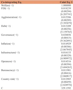
So from the two methods of co-integration (Pedroni residual co-integration test, Kao residual co-integration test) reveals that the variables are co-integrate. On the evidence of co-integrating relationship, a VECM is estimated to model the long run causality and short run dynamics. The purpose of VECM model is to indicate the speed of adjustment from the short run equilibrium to the long
run equilibrium state. The greater the coefficient of the parameter
the higher the speed of adjustment of the model from short runs to long run.
From the Table 6, the first model (details in the Appendix Table 1) is the main consideration where the welfare is the dependent variable.
First model specification = D(Welfare) = C(1)* (Welfare(−1) −0.194788256127*FDI(−1)−0.398426932314*Agglomeration( −1)+15.198624391828*Debt(−1)−12.198234621453*Govt(−1) +23.031842951672*Inflation(−1)−19.36789215*Infrastructure( −1)+11.728193174235*Open(−1)−14.832566170912*Bureaucr acy(−1)+22.029901479319*CountryRisk(−1)+C(2)*D(Welfare( −1))+C(3)*D(welfare(−2))+C(4)*D(FDI(−1))+C(5)*D(FDI(−2) )+C(6)*D(Agglomeration(−1))+C(7)*D(agglomeration(−2))+C (8)*D(Debt(−1))+C(9)*D(Debt(−2))+C(10)*D(Governance(−1)) +C(11)*D(Governance(−2))+C(12)*D(Inflation(−1))+C(13)*D (Inflation(−2))+C(14)*D(Infrastructure(−1))+C(15)*D(Infrastru cture(−2))+C(16)*D(Open(−1))+C(17)*D(Open(−2))+C(18)*D (Bureaucracy(−1))+C(19)*D(Bureaucracy(−2))+C(20)*D(Coun try Risk(−1))+C(21)*D(Country Risk(−2))+C(22).
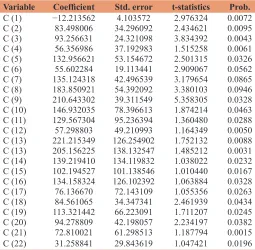
The following Table 7 interprets the first model.
Here C (1) means speed of adjustment towards long run equilibrium
but it must me significant and the sign must be negative. There is
long run causality from the variables such as FDI, agglomeration,
debt, governance, inflation, infrastructure, openness, bureaucracy,
and country risk. It interprets that the independent variables such
as FDI, agglomeration, debt, governance, inflation, infrastructure, openness, bureaucracy and country risk have an influence on the
dependent variable such as welfare.
The different variables like FDI, agglomeration, debt, governance,
inflation, infrastructure, openness, bureaucracy and country risk have an influence on the dependent variable such as welfare in the
short run. For measuring this Wald Statistics is being used. Here,
C(4)=C(5)=0 meaning that there is no short run causality running from FDI to welfare. C(6)=C(7)=0 meaning that there is no short run causality running from agglomeration to welfare. C(8)=C(9)=0
meaning that there is no short run causality running from debt to
welfare. C(10)=C(11)=0 meaning that there is no short run causality running from governance to welfare. C(12)=C(13)=0 meaning that there is no short run causality running from inflation to welfare. C(14)=C(15)=0 meaning that there is no short run causality running from infrastructure to welfare. C(16)=C(17)=0 meaning that
there is no short run causality running from openness to welfare.
C(18)=C(19)=0 meaning that there is no short run causality running from bureaucracy to welfare. C(20)=C(21)=0 meaning that there is
no short run causality running from country risk to welfare.
From the Table 8, it is explore that the P values of each of the independent variables are <5%. It means that there is a short run
causality running from the variables like FDI, agglomeration, debt,
governance, inflation, infrastructure, openness, bureaucracy and
country risk to welfare.
Table 6: Vector error correction model
Co-integrating Eq. Coint Eq. 1
Welfare(−1) 1.000000
FDI(−1) 0.018239
(0.00294) [6.203741]
Agglomeration(−1) 0.015586
(0.00289) [5.393079]
Debt(−1) 0.013209
(0.00256) [5.159765]
Governance(−1) 0.038856
(0.00415) [9.362891]
Inflation(−1) 0.014929
(0.00386) [3.867845]
Infrastructure(−1) 0.016153
(0.00329) [4.909972]
Openness(−1) 0.014516
(0.00394) [3.684263]
Bureaucracy(−1) 0.011901
(0.00416) [2.860817]
Country risk(−1) 0.012985
(0.00459) [2.828976]
C 329.1592
Table 5: Kao residual co-integration test
Kao residual
co-integration test t-statistic Prob.
ADF −3.291844 0.0028
Residual variance 2193.654
According to the Panel dynamic least squares method (DOLS), it is
seen that if the FDI goes up by 1 unit the welfare goes up 0.018675.
On the other hand in the case of agglomeration the paper has also found that if agglomerations have increased 1 unit then welfare
also has increased 0.184572. Reduction of debt 1 unit, the welfare has increased 0.124457. Increased of governance 1 unit, welfare has increased 0.152892.Reduction of inflation 1 unit, welfare has increased 0.115223. On the other hand, the paper has also explore
that if the improving the infrastructure 1 unit, welfare has increased
0.135191. In the case of openness variable, 1% increasing openness, welfare has increased 0.195623. Reduction of bureaucracy by 1%, the welfare goes up 0.115985 along with the reduction of 1% of country risk, welfare has increased 0.016218 (Table 9).
From the method of fully modified least square (FMOLS) it is seen that if the FDI goes up by 1 unit the welfare goes up 0.027956.
On the other hand in the case of agglomeration the paper has seen that if agglomerations have increased 1 unit then welfare has
increased 0.110327. The other independent variable debt has found that reduction of debt 1 unit, the welfare has increased 0.078451. Increased of governance 1 unit, welfare has increased 0.091872. Reduction of inflation 1 unit, welfare has increased 0.107263.
On the other hand, the paper has seen that if the improving the
infrastructure 1 unit, welfare has increased 0.111348. In the case of
openness variable, 1% increasing openness, welfare has increased
0.130955. If the bureaucracy diminishes by 1%, the welfare goes up 0.108327. Reduction of 1% of country risk, welfare has increased 0.079931.
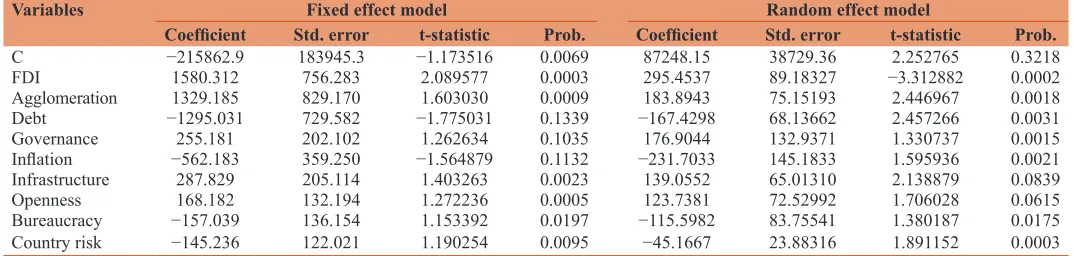
According to the fixed effect model the FDI variable is significant. Here the probability value is <5%, it means that FDI is significant variable to explain welfare. Agglomeration variable is significant because the probability value is <5%, it interprets that FDI is significant variable to explain welfare. Debt variable is not significant because the probability value is not <5%, it means that debt is not significant variable to explain welfare. Governance and inflation variable is not significant. Here the probability value is not <5%, it means that governance variable and inflation is not significant variable to explain welfare. Infrastructure variable is significant. Here the probability value is <5%, it means that infrastructure variable is also significant variable to explain welfare. Openness variable is also found significant because the probability value is <5%, it means that openness is significant variable to explain welfare. Bureaucracy variable is also found significant because the probability value is <5%, it means that bureaucratic variable is significant variable to explain welfare. Country risk variable is significant. Here the probability value is <5%, it means that country risk is significant variable to explain
welfare (Table 10).
From the random effect model, FDI variable is significant. Here the probability value is <5%, it means that FDI is significant variable to explain welfare. Agglomeration variable is significant because the probability value is <5%, it interprets that FDI is significant variable to explain welfare. Debt variable is significant because the probability value is not <5%, it means that debt is not significant variable to explain welfare. Governance and inflation variable is also found significant. Here the probability value is <5%, it means
that government variable and inflation is significant variable to explain welfare. Infrastructure variable is not significant. Here the probability value is not <5%, it means that infrastructure variable is not significant variable to explain welfare. Openness variable is not significant because the probability value is not <5%, it means that openness is not significant variable to explain welfare. Bureaucratic variable is also found significant because the probability value is <5%, it means that bureaucratic variable is significant variable to explain welfare. Country risk variable is significant. Here the probability value is <5%, it means that country risk is significant variable to explain welfare.
5. CONCLUSION
FDI escalates the economic advancement by improving the productivity of the labor forces through the inception of modern and sophisticated technology especially for the developing country.
The main substantive explore is that FDI that makes a significant and positive impact over the exploration of the welfare in the
developing countries. Host countries government accentuate on
extinguishing the multitudinous trade related impediment for the
purpose of unrestricted movement of FDI and also the government needs to establish a constructive and commensurate procedures and
Table 7: Model specification one
Variable Coefficient Std. error t-statistics Prob.
C (1) −12.213562 4.103572 2.976324 0.0072
C (2) 83.498006 34.296092 2.434621 0.0095
C (3) 93.256631 24.321098 3.834392 0.0043
C (4) 56.356986 37.192983 1.515258 0.0061
C (5) 132.956621 53.154672 2.501315 0.0326
C (6) 55.602284 19.113441 2.909067 0.0562
C (7) 135.124318 42.496539 3.179654 0.0865
C (8) 183.850921 54.392092 3.380103 0.0946
C (9) 210.643302 39.311549 5.358305 0.0328
C (10) 146.932035 78.396613 1.874214 0.0463
C (11) 129.567304 95.236394 1.360480 0.0288
C (12) 57.298803 49.210993 1.164349 0.0050
C (13) 221.215349 126.254902 1.752132 0.0088
C (13) 205.156225 138.132547 1.485212 0.0031
C (14) 139.219410 134.119832 1.038022 0.0232
C (15) 102.194527 101.138546 1.010440 0.0167
C (16) 134.158324 126.102392 1.063884 0.0328
C (17) 76.136670 72.143109 1.055356 0.0263
C (18) 84.561065 34.347341 2.461939 0.0434
C (19) 113.321442 66.223091 1.711207 0.0245
C (20) 94.278809 42.198057 2.234197 0.0382
C (21) 72.810021 61.298513 1.187794 0.0015
C (22) 31.258841 29.843619 1.047421 0.0196
Table 8: Wald statistics
Independent variable Hypothesis Prob.
FDI C (4)=C (5)=0 0.0008
Agglomeration C (6)=C (7)=0 0.0004
Debt C (8)=C (9)=0 0.0002
Governance C (10)=C (11)=0 0.0003
Inflation C (12)=C (13)=0 0.0007
Infrastructure C (14)=C (15)=0 0.0005
Open C (16)=C (17)=0 0.0002
Bureaucracy C (18)=C (19)=0 0.0001
program for the uninterrupted engagement of the foreign firms to
strengthening the welfare accumulation for the host countries that indubitably assists to propagate the socio-economic and macro-economic utility of the developing countries.
REFERENCES
Anand, S., Sen, A. (2000), Human development and economic sustainability. World Development, 28(12), 2029-2049.
Arcelus, F.J., Sharma, B., Srinivasan, G. (2005), Foreign capital flows and the efficiency of the HDI dimensions. Global Economy Journal, 5(2), 1058-1060.
Asiedu, E. (2002), On the determinants of foreign direct investment
to developing countries: Is Africa different? World Development,
30(1), 107-119.
Bain, J.S. (1951), Relationship of profit rate to ındustry concentration in American manufacturing, 1936-1940. Quarterly Journal of
Economics, 65, 293-324.
Barrell, R., Pain, N. (1997), Foreign direct investment, technological
change and economic growth within Europe. Economic Journal,
107, 1770-1786.
Blomstrom, M., Kokko, A. (2003), Multinational corporations and
spillovers. Journal of Economic Surveys, 12(2), 1-31.
Borensztein, E., De Gregorio, J., Lee, J.W. (1998), How does foreign direct investment affect economic growth? Journal of International
Economics, 45(1), 115-127.
Botric, V., Skuflic, L. (2006), Main determinants of foreign direct ınvestment in the Southeast European countries. Transition Studies Review, 13(2), 359-377.
Buckley, P.J. (1990), Problems and developments in the core theory of ınternational business. Journal of International Business Studies, 21(4), 657-665.
Cernat, L., Vranceanu, R. (2002), Globalization and development: New
evidence from central and Eastern Europe. Comparative Economic Studies, 44, 119-136.
Chakrabarti, A. (2001), The determinants of foreign direct investment:
Sensitivity analyses of cross-country regressions. Kyklos, 54, 89-113.
Chen, M. (1996), Competitor analysis and inter firm rivalry: Toward a
theoretical integration. Academy of Management Review, 21(1),
100-134.
Driffield, N., Girma, S. (2003), Regional foreign direct ınvestment and
wage spillovers: Plant level evidence from the U.K electronics
ındustry. Oxford Bulletin of Economics and Statistics, 65(4), 453-474.
Globerman, S., Shapiro, D. (2003), Governance infrastructure and US
foreign direct investment. Journal of International Business Studies, 34(1), 19-39.
Hansen, H., Rand, J. (2006), On the causal links between FDI and growth
in developing countries. World Economy, 29, 21-41.
Hymer, S. (1968), The efficiency (contradictions) of multinational corporations. American Economic Review, 60(2), 441-448.
Kakwani, N. (1981), Welfare measures: An international comparison. Journal of Development Economics, 8(1), 21-45.
Kersan-Skabic, I., Orlic, E. (2007), Determinants of FDI in CEE, Western balkan countries (ıs accession to the EU ımportant for attracting FDI? Economic and Business Review, 9(4), 333-350.
Konings, J. (2001), The effects of foreign direct ınvestment on domestic
firms: Evidence from firm and level panel data in emerging economies. Economics of Transition, 9(3), 619-633.
Lehnert, K., Benmamoun, M., Zhao, H. (2013), FDI ınflow and human development: Analysis of FDI’s ımpact on host countries’ social welfare and ınfrastructure. Thunderbird International Business
Review, 55(3), 285-298.
Li, X., Liu, X. (2005), Foreign direct ınvestment and economic growth: An ıncreasingly endogenous relationship. World Development, 33(3), 393-407.
Lucas, R. (1993), On the determinants of direct foreign ınvestment:
Evidence from East and Southeast Asia. World Development, 21(3),
391-409.
MacDougall, G.D.A. (1960), The benefits and costs of private investment from abroad: A theoretical approach. Economic Record, 36(73),
Table 9: Panel dynamic least squares and fully modified least square method
Variables Panel dynamic least squares method Fully modified least square method
Coefficient Std. error t-statistic Prob. Coefficient Std.error t-statistic Prob.
FDI 0.286751 2.82E-12 6.62E+03 0.0000 0.227956 3.47E-15 8.05E+07 0.0006
Agglomeration 0.184572 1.45E-11 1.27E+15 0.0000 0.110327 2.21E-05 4.99E+11 0.0003
Debt −0.124457 1.09E-09 1.14E+10 0.0000 −0.078451 1.27E-04 6.17E+09 0.0002
Governance 0.152892 1.11E-03 1.37E+18 0.0002 0.091872 1.25E-06 7.34E+07 0.0003
Inflation −0.115223 1.15E-07 1.00E+09 0.0004 −0.107263 1.43E-03 7.50E+09 0.0001
Infrastructure 0.135191 1.12E-11 1.20E+12 0.0000 0.111348 1.29E-07 8.63E+15 0.0000
Openness 0.195623 1.13E-10 1.73E+07 0.0000 0.130955 1.45E-08 9.03E+11 0.0000
Bureaucracy −0.115985 1.11E-09 1.04E+11 0.0000 −0.108327 1.37E-10 7.90E+11 0.0000
Country risk −0.016218 1.09E-12 1.48E+10 0.0000 −0.079931 1.57E-11 5.09E+09 0.0000
Table 10: Fixed effect model and random effect model
Variables Fixed effect model Random effect model
Coefficient Std. error t-statistic Prob. Coefficient Std. error t-statistic Prob.
C −215862.9 183945.3 −1.173516 0.0069 87248.15 38729.36 2.252765 0.3218
FDI 1580.312 756.283 2.089577 0.0003 295.4537 89.18327 −3.312882 0.0002
Agglomeration 1329.185 829.170 1.603030 0.0009 183.8943 75.15193 2.446967 0.0018
Debt −1295.031 729.582 −1.775031 0.1339 −167.4298 68.13662 2.457266 0.0031
Governance 255.181 202.102 1.262634 0.1035 176.9044 132.9371 1.330737 0.0015
Inflation −562.183 359.250 −1.564879 0.1132 −231.7033 145.1833 1.595936 0.0021
Infrastructure 287.829 205.114 1.403263 0.0023 139.0552 65.01310 2.138879 0.0839
Openness 168.182 132.194 1.272236 0.0005 123.7381 72.52992 1.706028 0.0615
Bureaucracy −157.039 136.154 1.153392 0.0197 −115.5982 83.75541 1.380187 0.0175
13-35.
McKenzie, G.W., Pearce, I.F. (1982), Welfare measurement: A synthesis.
The American Economic Review, 72(4), 669-682.
Mengistu, B., Adams, S. (2007), Foreign direct ınvestment, governance
and economic development in developing countries. Journal of Social, Political and Economic Studies, 32(2), 223-249.
Meyer, K. (2004), Perspectives on multinational enterprises in emerging
economies. Journal of International Business Studies, 3, 35-44.
Meyer, K., Sinani, E. (2009), When and where does foreign direct
investment generate positive spillovers? A meta-analysis. Journal
of International Business Studies, 40, 1075-1094.
Mirza, H., Giroud, A. (2003), Regionalization, foreign direct ınvestment and poverty reduction. Journal of the Asia Pacific Economy, 9(2), 223-248. Penrose, E. (1956), Foreign ınvestment and the growth of the firm. The
Economic Journal, 66(262), 220-235.
Phillips, P., Hansen, B. (1990), Statistical ınference in ınstrumental
variables regression with I(1) processes. Review of Economic
Studies, 57, 99-125.
Pyatt, G. (1987), Measuring welfare, poverty and inequality. The Economic Journal, 97(386), 459-467.
Rogers, M. (2004), Absorptive capacity and economic growth: How do countries catch up? Cambridge Journal of Economics, 28, 577-596. Zhang, K.H. (2001), What attracts foreign multinational corporations to
China? Contemporary Economic Policy, 19(3), 336-346.
Zhao, H. (2013), Technology imports and their impacts on the
enhancement of China’s indigenous technological capability. Journal
APPENDIX
T
ABLE
Err or corr ection W elfar e FDI GDP DEBT Govt. spend INFLA Infras Open Human Country riskCoint Eq. 1
−0.120295 2.560248 3.952673 −0.087613 0.189921 −0.157205 1.764339 0.187622 0.079472 0.188152 (0.06475) (1.17635) (2.01852) (0.03284) (0.07105) (0.09521) (1.27042) (0.05988) (0.04968) (0.09621) [−1.857837] [2.176433] [1.958203] [2.667874] [2.673061] [1.651 139] [1.388784] [3.133329] [1.599677] [1.955638] D {W elfare(−1)} −0.015728 0.005373 0.321562 0.013558 0.236619 0.958924 0.074182 0.298491 0.091331 0.052183 (0.0138) (0.00829) (0.1 1892) (0.02615) (0.03752) (0.71682) (0.03916) (0.33492) (0.08629) (0.06518) [−1.139710] [0.648130] [2.704019] [0.518470] [6.306476] [1.337747] [1.894330] [0.891230] [1.058419] [0.800598] D {W elfare(−2)} −0.183953 0.451986 0.598213 0.036721 0.088394 0.586392 0.274893 0.008276 0.023410 0.814194 (0.14272) (0.41 137) (0.43183) (0.04903) (0.09462) (0.34662) (0.21684) (0.00294) (0.03625) (0.73416) [−1.288908] [1.098733] [1.385297] [0.748949] [0.934199] [1.691743] [1.267722] [2.814965] [0.645793] [1.109014] D {FDI(−1)} 0.709755 0.009427 0.02981 1 0.064192 0.779801 0.851936 0.521964 0.416580 0.461925 0.033184 (0.52214) (0.00776) (0.05418) (0.08462) (0.54825) (0.95193) (0.48962) (0.07419) (0.26193) (0.04518) [1.359319] [1.214819] [0.550221] [0.758591] [1.422345] [0.894956] [1.066059] [5.615042] [1.763543] [0.734484] D {FDI(−2)} 0.156209 0.076342 0.029518 0.970928 1.037782 1.075329 0.821673 0.008294 0.023195 0.042819 (0.1 1774) (0.01835) (0.04513) (0.83625) (0.85138) (0.92816) (0.29136) (0.00569) (0.01988) (0.03414) [1.326728] [4.160326] [0.654066] [1.161049] [1.218941] [1.158559] [2.820129] [1.457644] [1.166785] [1.254217] D {Agglomeration(−1)} 1.856616 1.434628 0.821942 0.694552 0.002988 0.721734 0.621592 0.490855 0.551929 0.351986 (0.43759) (0.97425) (0.71661) (0.84291) (0.00964) (0.68549) (0.25730) (0.07629) (0.38216) (0.32146) [4.242820] [1.472546] [1.146986] [0.823993] [0.309958] [1.052873] [2.415825] [6.433814] [1.444235] [1.094960] D {Agglomeration(−2)} 0.973326 0.008735 0.093195 0.568325 1.078842 0.884216 0.741829 0.008094 0.498615 0.628125 (0.65198) (0.00946) (0.08215) (0.44528) (0.95884) (0.93198) (0.62194) (0.00629) (0.41294) (0.35147) [1.492870] [0.929255] [1.134449] [1.276331] [1.125153] [0.948749] [1.192766] [1.286804] [1.207475] [1.787136] D {Debt(−1)} 0.076295 0.784516 1.179037 0.872902 0.937748 0.004561 0.598236 0.093887 0.201552 0.298417 (0.04182) (0.28925) (0.96772) (0.95182) (0.95828) (0.00365) (0.41837) (0.07725) (0.07053) (0.32156) [1.824366] [2.712242] [1.218365] [0.917087] [0.978574] [1.249589] [1.429920] [1.215365] [2.857677] [0.928028] D {Debt(−2)} 1.167925 1.135198 0.098337 0.397451 0.761825 0.689243 0.008296 0.003966 0.006718 0.182643 (1.35266) (0.93821) (0.17527) (0.48942) (0.39832) (0.44183) (0.02916) (0.00437) (0.00821) (0.27182) [0.863428] [1.209961] [0.561060] [0.812085] [1.912595] [1.559973] [0.284499] [0.907551] [0.818270] [0.671926] D {Governances(−1)} 0.298142 0.006741 0.079183 0.008726 0.198563 0.063184 0.512783 0.901812 0.008321 0.004839 (0.08563) (0.00863) (0.05981) (0.00782) (0.08126) (0.05610) (0.08871) (0.28391) (0.58920) (0.00542) [3.481747] [0.781 112] [1.323909] [1.1 15856] [2.443551] [1.126274] [5.780441] [3.176400] [0.014122] [0.892804] D {Governance S(−2)} 0.853442 0.794831 0.006744 0.008125 0.078183 0.524631 0.197533 0.947718 0.082183 0.246218 (0.38498) (0.56159) (0.00729) (0.00939) (0.08326) (0.39183) (0.07320) (0.75192) (0.72551) (0.33192) [2.216847] [1.415322] [0.925102] [0.865282] [0.939022] [1.338923] [2.698538] [1.260397] [0.1 13276] [0.741799] D {Inflation(−1)} 0.196749 0.005642 0.379721 0.002947 0.662916 0.458231 0.328719 0.043170 1.076618 0.125579 (0.09216) (0.00521) (0.09822) (0.00375) (0.09833) (0.37829) (0.09217) (0.53930) (0.95183) (0.05613) [2.134863] [1.082917] [3.866025] [0.785866] [6.741747] [1.21 1322] [3.566442] [0.080048] [1.131 103] [2.237288] D {Inflation(−2)} 0.491503 0.025774 0.068352 0.416382 0.941829 0.432015 0.387292 0.698364 0.921712 0.428694 (0.21882) (0.05375) (0.05219) (0.26941) (0.58762) (0.58259) (0.41256) (0.45283) (0.93151) (0.06352) [2.246152] [0.479516] [1.309676] [1.545532] [1.602785] [0.741542] [0.938753] [1.542221] [0.989481] [6.748960] D {Infrastructure(−1)} 0.051603 0.004672 0.052183 0.952981 0.082951 0.067182 0.007284 0.072903 0.451662 0.048625 (0.03929) (0.07528) (0.07943) (0.66382) (0.07682) (0.04961) (0.00298) (0.08294) (0.58021) (0.03516) [1.313387] [0.062061] [0.656968] [1.435601] [1.079809] [1.354202] [2.444295] [0.878984] [0.778445] [1.382963] D {Infrastructure(−2)} 0.039156 0.731946 0.498325 0.764092 0.064798 0.212412 0.091829 0.562904 0.006518 0.274512 (0.02158) (0.46675) (0.07131) (0.34839) (0.05541) (0.43192) (0.05683) (0.09418) (0.00531) (0.05619) [1.814457] [1.568175] [6.988150] [2.193208] [1.169427] [0.491785] [1.615854] [5.976895] [1.227495] [4.885163] Appendix Table 1: Differ