General Equilibrium Modeling for Economic Policy Analysis

Issues

ISSN: 2146-4138

available at http: www.econjournals.com

International Journal of Economics and Financial Issues, 2019, 9(4), 25-36.

General Equilibrium Modeling for Economic Policy Analysis

Truong Hong Trinh*

Department of Finance,University of Economics - The University of Danang, Vietnam. *Email: [email protected]

Received: 23 April 2019 Accepted: 20 June 2019 DOI: https://doi.org/10.32479/ijefi.8164

ABSTRACT

This paper explores the value concept that is important in determining the relationship between demand and supply, and resource allocation in the economy. From value creation perspective, the value concept is redefined to explain value creation and value distribution in the economy. Based on this value concept, the value added method is used for gross domestic product (GDP) measurement that is also used as the objective function in the general equilibrium model. The starting point in general equilibrium modeling is the understanding on the structure and the flows of the economy, in which the general equilibrium mechanism relies on market equilibriums and macro balances. The simulation experiment is used to conduct economic policies from the changes in target sector structure and the combinations of macro closures in the hypothetical economy. The paper contributes a conceptual framework in general equilibrium modeling for economic policy analysis as a good start to understand the more complex general equilibrium models. Keywords: Value Concept, Market Equilibrium, General Equilibrium, Policy Analysis, Economic Growth

JEL Classifications: C60, D46, D58, O20

1. INTRODUCTION

Economic growth is always the central topic in economic literature. Many researchers attempt to identify driven factors on the economic growth that forms the base of economic growth theories. To deal with this problem, economists must understand general equilibrium and GDP measurement of the economy. It also requires a standard tool to analyse economic policies on the economic growth and transition.

In earlier literature, economists attempt to explore the value concept that plays an important role in determining relationship between demand and supply, and resource allocation in the economy. Neoclassical economists have used this value concept to explain market equilibrium in terms of supply and demand (1890) and general equilibrium as a means of integrating both the effects of the demand and supply side forces in the whole country (Walras, 1874). From this theoretical base, Arrow and Debreu (1954) developed algebraic concepts and equilibrium conditions for general equilibrium model. The general equilibrium model

is built upon institutions (households, enterprises, governments, and rest of world), markets (commodity markets, factor markets, and financial markets), and macro balances (internal balance, government balance, and external balance). In recent literature, economists develop computable general equilibrium (CGE) models to study how an economy reacts to the changes in economic policies.

In order to develop computable general equilibrium models, economists need to define objective functions and equilibrium conditions. For the objective functions, Lofgren et al. (2002) and Sue Wing (2009) employed the Cobb Douglas production and utility functions in their general equilibrium models. Meanwhile, the Stone – Greary and the CES (Constant Elasticity of Substitution) utility functions are employed by Hosoe et al. (2010) and Sue Wing (2009), respectively. For equilibrium conditions, market clearance imposes a condition to equilibrate markets of commodities and resources with econometric techniques of CES (Constant Elasticity of Substitution) and CET (Constant Elasticity of Transformation). In addition, first order conditions are used for

production and consumption decisions to maximize firm profit and customer utility (Lofgren et al., 2002; Sue Wing, 2009; Hosoe et al., 2010). Since economists use econometric techniques and first order conditions to drive the price system for market equilibriums, the CGE models may ignores market behaviors in nature. The big challenges in CGE modeling involve GDP measurement, market price system, and macro balance considerations.

For that reason, this paper explores the value concept and defined the utility function with incorporation of value and price. From this theoretical base, the value added method is used for GDP measurement that is used as the objective function in the general equilibrium model with constraints of market equilibriums and macro balances. The simulation experiment is designed to conduct economic policies under the changes in target sector structure and macro balances.

2. VALUE CONCEPT

The concept of value has a very long history in economic and philosophical thought that attempt to explain two notions: value-in-use (value) and value-in-exchange (price). The difference between value-in-use and value-in-exchange is important to form the base of value theories. Classical economics relies on the labor theory of value with the work of Smith (1776) and Ricardo (1821). Classical economists argued that the value of a commodity come from the amount of labor spent to produce and bring it to market for exchange. Neoclassical economics relies on the utility theory of value that stems from a subjective valuation by an economic agent on the worth of a commodity. Neoclassical economists intended to conceptualize utility and construct a theory of price in keeping with the utilitarianism of Bentham (1789) and Dupuit (1844). Later, Jevons (1871) and Menger (1871) developed a new tool of marginal analysis as a means of understanding the value concept.

Most economists tried to make a clear distinction between value and price of a commodity. Baier (1966) offered a broader

definition such as “value is the capacity of a commodity or activity to satisfy a need or provide a benefit to a person or legal entity.” Value is something which is perceived and evaluated at the time of consumption (Wikström, 1996; Woodruff and Gardial, 1996; Vargo and Lusch, 2004; Grӧnroos, 2008). There is a common understanding that value is created in the users’ processes as value-in-use (Grönroos, 2011; Trinh, 2018). Since value is more appreciate than utility in explanting value creation and value distribution in today’s society and economy, the value concept needs to redefine to form a new theory of value, in which the theory of value should be constructed upon a law of diminishing marginal value (Trinh, 2014). The theory of value is the foundation to understand and explain relationship between demand and supply, resource allocation in the economy. From this theoretical base, the utility function is defined with the incorporation of value and price (Trinh et al., 2014) as follows.

TU = × = −u Q

(

v p

)

× =Q TV TR− (1)

Where, v, p, and u are unit value, unit price, and unit utility, respectively. TV, TR, and TU are total value, total revenue, and total utility, respectively.

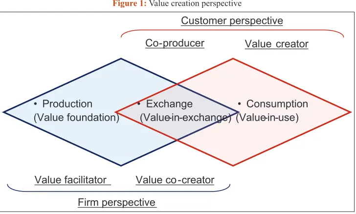
From the value creation perspective, the value creation system involves three processes of production, exchange, and consumption as in Figure 1. Value is always created in the consumption process, price is determined in the exchange process. The price plays as a role of value distribution between the firm and the customer.

In the firm perspective, the firm takes on the role of value facilitator, and also joins in the consumption process as a value co-creator. Firm’s production function is defined under the form of Cobb Douglas production function as follows:

(

)

1 1

1, 1 1 1 1

= = × ×

Q f K L A K L (2)

Co-producer

Customer perspective

• Production

(Value foundation) • Exchange(Value-in-exchange) (Value-in-use)• Consumption

Value facilitator Value co-creator Firm perspective

Value creator

Source: Adapted from Grӧnroos and Voima (2012), Trinh (2017a)

Where, Q is total output of production. A₁ is firm’s total factor productivity. K₁and L₁are firm capital and firm labor, respectively. α₁, β₁, are the output elasticities of production input factors.

By using the least-cost combination of production inputs, firm’s cost function (TC₁) can be determined as a function of output, depending on input prices and the parameters of the firm’s production function as follows:

TC₁=K₁×w_K1+ ×L₁ w_L1 (3) Where, TC₁ is firm’s total cost, w_k1 and w_L1 are unit costs of firm capital and firm labor.

Firm’s profit function is determined by the following formula.

1 1

1 1 1

= − = × − × K − × L

II TR TC p Q K w L w ₍₄₎

Where, II is firm profit and TR is total revenue (TR= ×p Q).

In the customer perspective, the customer is always a value creator. The customer also takes part in the production process as a co-producer. Since the value is created in the consumption process, customer capital (K₂) and customer labor (L₂) are added in the consumption function as follows:

Q= f K L

(

2, 2

)

= A2×K2α2×Lβ22 (5)

Where, Q is total output of consumption. A₂ is customer’s total factor productivity. α₂, β₂,are the output elasticities of consumption input factors.

By using the least-cost combination of consumption inputs, customer’s cost function (TC₂) can be determined as a function of output, depending on input prices and the parameters of the customer’s consumption function as follows:

TC₂ =K₂×w_K2+L₂×w_L2 (6) Where, TC₂ is customer’s total cost, w_K2and w_L2are unit costs of customer capital and customer labor.

Customer’s utility function is determined by the following formula.

U=TU TC− 2 = −

(

v p

)

× −Q K2×w_K2 −L2×w_L2 (7) Where, U is customer utility and TU is total utility (TU = u × Q = (v – p) × Q).

From the value creation perspective, value is created in the consumption process, both firm cost and customer cost include in value creation system. The total cost function and the net value function are determined as follows:

TC TC= 1+TC2 =K1×w_K1+ ×L1 w_L1+K2×w_K2+L2×w_L2 (8)

1 1

2 2

1 1 2

2

× + × +

 

= + = × −_{ }= −

× + ×

 

K L

K L

K w L w K

V U v Q TV TC w L w

 ₍₉₎

Where, V is net value, TV is total value (TV = v × Q) and TC is total cost. w_K1and w_L1are unit costs of firm capital and firm labor. w_K2and w_L2are unit costs of customer capital and customer labor.

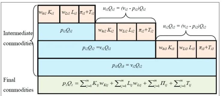
In economics, the value concept has influence on how GDP is measured. GDP is measured by valuating everything that is produced and added all value together. The value added method is used to determine production value of final commodity in the industry i (p_iQ_i) through production and exchange processes of intermediate commodities as illustrated in Figure 2. Total production value is formed by summing up final commodity’s production value of all industries in the economy.

For the intermediate exchange processes, intermediate firms play dual role of the firm and the customer. In the initial exchange process, firms provide the commodities to customers. Firm profit (P_i1) and customer utility (U_i1) are determined as follows:

1 1

1= 1× 1− 1× i − 1× i − 1

i pi Qi Ki wK Li wL Ti

 (10)

U_i1=

(

v_i1−p_i1

)

×Q_i1−K_i2×w_Ki2−L_i2×w_Li2−T_i2 (11) The customer then plays a role of the firm in the next exchange process. The customer utility (U_i1) in the initial exchange process is also the firm profit (P_i2) in the next exchange process.

Source: Trinh (2017a)

2 2

2 = 2× 2− 2× i − 2× i − 2

i pi Qi Ki wK Li wL Ti

 (12)

U_i2 =

(

v_i2−p_i2

)

×Q_i2−K_i3×w_Ki3−L_i3×w_Li3 −T_i3 (13) For the final exchange process, the final consumers buy the final commodities from the last exchange processes. Firm profit (P_im) is given as follows:

(

−1 −1

)

= × − × − × _im− × _im−

im pim Qim pim Qim Kim wK Lim wL Tim



(14)

Total profit (net value) of industry i is determined through the following formula.

1 1 1 1

= = = =

= × − × − × −

∑

∑

ij

∑

ij

∑

m m m m

ij im im ij K ij L ij

j j j j

p Q K w L w T

 (15)

From above formula, gross domestic product of industry i

p_i Q_i I_i p_im Q_im I_ij

j m × + = × +         =

∑

1

is defined as a sum of

production value (p_i×Q_i) and capital investment (I_i), in which total

expenditure p_im Q_im I_ij j m × +         =

∑

1

is equal to total income

1 1 1 1 1

= = = = =

 

× + × + + +

 

 



∑

ij

∑

ij

∑ ∑ ∑



m m m m m

ij K ij L ij ij ij

j j j j j

K w L w  T I , in which

I_ij j m =

∑

1

is capital investment of industry i. By setting

K_i w_Ki K_ij w j m Kij × = × =

∑

1

, L_i w_Li L_ij w j m Lij × = × =

∑

1 , 1 , m i ij j   = =

∑

T_i T_ij j m = =

∑

1

, I_i I_ij j m = =

∑

1

, gross domestic product of industry i can be expressed as follows:

+ = × _i + × _i + + +

i i i i K i L i i i

p Q I K w L w  T I (16)

Gross domestic product (GDP) of the economy with n industries is determined as follows:

GDP p_i Q_i I

i n i i n = × + = =

∑

∑

1 1 (17)

1 1 1 1 1

= = = = =

=

∑

n i× K_i+

∑

n i× L_i +

∑ ∑ ∑

n i+ n i+ n i

i i i i i

GDP K w L w  T I (18)

By setting

1 1 1 1

= = = =

= + −

∑

n Fi

∑ ∑ ∑

n i n i n i

i i i i

S  I D , in which S_Fi

i n =

∑

1 is

firm savings and D_i i

n

=

∑

1

is capital depreciation. Thus, GDP from

Equation (18) can be rewritten as follows:

GDP K_i w L w S D T i n K i i n L Fi i n i i n i i n i i = × + × + + + = = = = =

∑

∑

∑ ∑ ∑

1 1 1 1 1

(19)

From Equation (17), setting PQ p_i Q_i i n = × =

∑

1

and I I_i

i n = =

∑

1 , in

which total expenditure on final commodities

( )

PQ includes

personal expenditure (C), government expenditure (G), and net export (NX). GDP measurement under the expenditure approach can be expressed as follows:

GDP C G I NX= + + + (20)

F r o m E q u a t i o n ( 1 9 ) , s e t t i n g LW_L L_i w_Li i n = × =

∑

1 ,

KW_K K_i w_Ki i n = × =

∑

1

, S_F S_Fi i n = =

∑

1

, D D_i

i n = =

∑

1

, and T Ti i n = =

∑

1 ,

GDP measurement under the income approach can be expressed as follows:

GDP KW= _K+LW_L+S_F + +D T (21) GDP is measured through total income that includes capital interest (KW_K), labor wage (LW_L), firm savings (S_F), capital depreciation (D), tax and subsidy (T).

3. GENERAL EQUILIBRIUM MODEL

The starting point in general equilibrium modeling is the understanding on the basic structure and key flows of the economy. How does government policy influence GDP? The structure of the economy includes three main elements: markets, institutions, and macro balances. Figure 3 illustrates a basic structure of the economy that shows how institutions (households, enterprises, governments, and rest of world) interact in markets (commodity markets, factor markets, and financial markets) under macro balances (internal balance, government balance, and external balance). The circular flow diagram is a simplified representation the structure of the economy that shows fund flows, commodities, and factors through the economy. The underlying principle is that fund inflow into each market or institution is equal to fund outflow of that market or institution.

The economy contains four institutions: households, enterprises, governments, and rest of world.

Households receive income from factor markets in form of wages, profit, interest, and rent fees. Households spend for commodities from commodity markets. Households may send their saving or borrow money for their spending from financial markets.

Enterprises receive revenue from providing goods or services for households, governments, rest of world (ROW) on commodity markets. Enterprises also spend on costs of capital and labor on factor markets. Enterprises also need a required capital for their investment. Enterprises may send their profits to financial markets or make loans from financial markets.

borrow money for their fiscal deficit from financial markets or send their fiscal surplus to financial markets. In addition, government returns a portion of the money it collect from tax in form of subsidies that supports for enterprises and households.

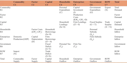
The fund flows of the economy are presented in a social accounting matrix (SAM). SAM provides economic data for CGE models, the CGE simulations update experimental results into SAM for economic policy analysis. SAM is an accounting framework that assigns numbers to the inflow (income) and outflow (expenditure) in the circular flow diagram. A SAM is laid out as a square matrix in which each row and column is called an “account”. Table 1 shows the SAM that corresponds to the circular flow diagram in

Figure 3. Each of the boxes in the diagram is an account in the SAM. Each cell in matrix presents a fund flow from a column account to a row account. The underlying principle of double-entry accounting requires that for each account in the SAM, fund inflow (total income) equals fund outflow (total expenditure).

Commodities are supplied by domestic production [R5-C1] and imported from ROW [R7-C1]. This total supply must be equal to total demand that includes personal expenditure [R1-C4], capital investment [R1-C5], government expenditure [R1-C6], and export [R1-C7]. Factors of production are supplied by households [R4-C2] and enterprises under capital depreciation [R5-C2]. This factor supply is also equal to production costs

Table 1: Basic structure of a SAM

Commodity

C1 FactorC2 CapitalC3 HouseholdsC4 EnterprisesC5 GovernmentC6 ROWC7 Total Commodity

R1 Personal Expenditure

(C)

Capital Investment (I)

Government Expenditure (G)

Export

(X) TotalDemand

Factor

R2 Production Costs

(KW_K+LW_L+D)

Factor Demand

Capital

R3 Household Lendings

(Sc>0)

Firm Lendings

(П > 0) Fiscal Surplus(G < T) Trade Surplus (X < N)

Capital Demand

Households

R4 Factor Costs(KWK+LWL)

Household Borrowings (Sc<0)

Personal Subsidy (S_bP)

Household Inflow Enterprises

R5 Domestic Production (GDP) Capital Depreciation (D)

Firm Borrowings (П < 0)

Firm Subsidy

(S_bF) Enterprise Inflow Government

R6 Fiscal Deficit

(G>T)

Personal Tax

(T_P) Firm Tax(T_F) Government Inflow ROW

R7 Import(N) Trade Deficit (X>N)

ROW Inflow Total Commodity

Supply FactorSupply Capital Supply Household Outflow Enterprise Outflow Government Outflow ROW Outflow

Production Costs

Capital Investment

Capital Depreciation Firm Tax

Factor Costs

Personal Tax

Firm Borrowings Household Borrowings Fiscal Deficit Trade Surplus

Personal Subsidy Firm Subsidy

Firm Lendings Household Lendings Fiscal Surplus

Trade Deficit Export Import

Government Expenditure Enterprises Households Government

ROW

Financial Markets

Commodity Markets

Factor Markets

Domestic

Production

Personal Expenditure

[R2-C5] demanded by enterprises. Funds are supplied by household savings [R3-C4] and firm profits [R3-C5]. The funds are also demanded by government [R6-C3] and rest of world [R7-C3] for their deficits, household borrowings [R4-C3], and firm borrowings [R5-C3].

Households receive income from providing capital and labor [R4-C2], and used for personal expenditure [R4-C1]. Households may send their savings to financial markets [R3-C4] or borrow their deficit from financial markets [R4-C3]. Enterprises pays out for production costs [R2-C5], capital investment [R1-C5], and firm tax [R6-C5]. Enterprises also receive revenue from domestic production [R5-C1] and capital depreciation [R5-C2]. Enterprises may send their profit to financial markets [R3-C5] or borrow money from financial markets [R5-C3]. Government collects tax from households [R6-C4] and enterprises [R6-C5], and returns personal subsidy [R4-C6] and firm subsidy [R5-C6]. It also spends for government expenditure [R1-C6]. Government either borrows money for fiscal deficit [R6-C3] from financial markets, or sends fiscal surplus to financial markets [R3-C6]. ROW pays for export [R1-C7] and receives from import [R7-C1]. ROW send trade surplus [R3-C7] to financial markets, or borrow trade deficit [R7-C3] from financial markets.

Since SAM links economic data from national accounts, it is a useful tool to present the economy picture of a country. SAM is built upon market equilibriums and macro balances that will be reestablished under economic policy or economic shock. There are three equilibriums of commodity market, factor markets, and financial markets in which market supply is equal to market demand. The economy is constructed under macro balances including government balance, external balance, and internal balance. In fact, it will never understanding the economy until understanding on macro balances.

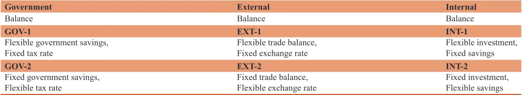
Government balance is a constraint choice between government savings (the difference between government revenue and government expenditure) and tax rates. Closure (GOV-1) is that government savings is a flexible residual while all tax rates are fixed. Under another closure (GOV-2), tax rates are adjusted endogenously to generate a fixed level of government savings.

External balance is a constraint choice between net export (the difference between export and import) and exchange rates. Closure (EXT-1) is that net export is a flexible, while the exchange rate is fixed. Under another closure (EXT-2), the exchange rate is flexible to generate a fixed level of trade balance (net export).

Internal balance is a constraint choice between investment drivers or saving drivers. Closure (INT-1) is that investment quantities are flexible, while savings is fixed. For another closure (INT-2), investment is fixed to generate a flexible level of saving.

Table 2 shows combinations of closure from macro balances. The proper choice between the different macro closures depends on the context of the policy analysis. There are 8 macro closures that are used to analyses changes in economic policy on the economic growth. The economic policies are proposed upon the combinations of macro closures.

In the real economy, the economy is expanded with economic policies, such as net export (NX), tax and subsidy (T), government expenditure (G), capital investment (I), and capital depreciation (D). Under conditions of market equilibriums and macro balances, the basic general equilibrium model is developed with main assumptions as follows:

1. Households (customers) consume m commodities with the same preference or consumption parameters.

2. Enterprises (producers) provide m identical commodities with the same production parameters.

3. The economy has m sectors, and each sector produces only one commodity.

4. Demand function is given for each commodity under the experiment.

5. Net export (NX), tax or subsidy (T), government expenditure (G), capital investment (I), and capital depreciation (D) are given parameters in the model.

In order to analyze changes in economic policy, the simulation experiment is carried out on the hypothetical economy with m

sectors, each sector produce an commodity (j = 1.m) by using total capital (K_j) and total labor (L_j). The demand function of a commodity j is defined as follows:

Price demand: pj= f Q

( )

j (22)

Market equilibrium condition imposes a condition to equilibrate total supply (Q_j) and total demand (Q_{cj +} Q_Gj + Q_NXj) for all commodities (j = 1.m).

Market equilibrium: Q_j =Q_Cj+Q_Gj+Q_NXj (23) Production function (Q_j) of commodity j is given as follows:

Production function: Q_{Sj =}A_j×Kα_jj _×Lβ_jj (24)

Table 2: The combinations of macro closures

Government External Internal

Balance Balance Balance

GOV-1 EXT-1 INT-1

Flexible government savings, Flexible trade balance, Flexible investment,

Fixed tax rate Fixed exchange rate Fixed savings

GOV-2 EXT-2 INT-2

Let’s put all in the CGE model that is presented under the following programming model. The objective function is to maximize GDP under the constraints of market equilibriums and macro balances.

The basic general equilibrium model:

MaxGDP P Q P Q P Q

EX I j j m Cj j j m Gj j j m NXj j j j m = × + × + × × + = = = =

∑

∑

∑

∑

1 1 1

1

(25)

Subject to

pj= f Q

( )

j ∀ =j 1..m (26)

Q_{j =}A_j×Kα_jj _×Lβ_jj _{∀ =}j _1..m (27)

Q_j =Q_Cj+Q_Gj+Q_NXj ∀ =j 1..m (28)

P_j×Q X_j= _j ∀ =j 1..m (29)

T -_j P Q A j m j Gj j m = =

∑ ∑

× ≥ 1 1 (30)

P_j Q_NXj EX B j m j × × ≤ =

∑

1 (31)

P_j Q _Gj P Q EX - T C j m j NXj j m j j j m × + × × ≥ = = =

∑

∑

∑

1 1 1

(32)

∀K , L P Q_{j j}, ,_{j j} , Q_Cj ∀ =j 1..m

Notations:

Indices:

j: index of sector (j = 1… m)

System parameters:

A_j: Total factor productivity of sector j w_Kj: Unit cost of capital of sector j w_Lj: Unit cost of labor of sector j α_j: Output elasticity of capital of sector j β_j: Output elasticity of labor of sector j

Policy parameters:

T_j: Tax and subsidy impose on sector j Q_NXj: Net export output of sector j

Q_Gj: Government expenditure output of sector j I_j: Capital investment of sector j

D_j: Capital depreciation of sector j X_j: Target GDP of sector j

EX_j: Ratio of export price and import price

A: Lower bound value of government balance

B: Upper bound value of external balance

C: Lower bound value of internal balance

Variables:

Q_j: Total production output of sector j Q_cj: Personal expenditure output of sector j P_j: Unit price of sector j

K_j: Total capital of sector j L_j: Total labor of sector j

The basic general equilibrium model is developed with the objective function of GDP that is built upon the value added method. The model is based on equilibrium of total supply and total demand as in Constraints (27) and (28), target sector structure as in Constraint (29), and macro balances as in Constraints (30), (31), and (32). The simulation experiment is carried out on the hypothetical economy with m sectors. Each sector j (j = 1.m) produces one commodity with total production output of Q_j (j = 1..m) by using total capital (K_j) and total labor (L_j). The domestic price for commodity j is given by the demand function P_j = f(Q_j). Net export price is adjusted with a ratio of

EX_j that depends on exchange rate, export price and import price for the commodity j.

In order to analyze changes in economic policy on the economy, policy constraints of (29), (30), (31), and (32) are added to the general equilibrium model. Constraint (29) sets a target structure of GDP for each sector of the economy(P_j × Q_j = X_j) (j = 1..m). Constraint (30) sets an lower bound value (A) for government balance, which is equal to government revenue (tax and subsidy)

T_j j m =

∑

        1

minus government expenditure P_j Q_Gj j m ×         =

∑

1 .

Constraint (31) sets an upper bound value (B) for external balance, which is equal to P_j Q_NXj EX

j m j × × =

∑

1

. Constraint (32) sets a l o w e r b o u n d v a l u e (C) f o r i n t e r n a l b a l a n c e

P_j Q _Gj P Q EX - T j m j NXj j m j j j m × + × ×         = = =

∑

∑

∑

1 1 1

which equals

subtraction of external balance P_j Q_NXj EX j m j × ×         =

∑

1 from

government balance T -_j P_j Q_Gj j m j m ×         = =

∑

∑

1 1

. Since GDP is not a

good indicator of economic welfare, but welfare relies on economic policies. By setting parameters and constraints of macro balances, economists may improve welfare of the economy or make the balance between GDP and welfare of the economy.

4. ECONOMIC POLICY ANALYSIS

In order to conduct economic policies, the simulation experiment assumes that the hypothetical economy has only three largest sectors (Agriculture, Industry, Services) (j = 3). Parameters of the economy are given in Table 3 and Table 4.

Table 4: Policy parameters of the economy

Sectors j Symbol Agriculture Industry Services

Tax and subsidy T_j 20 30 10

Capital investment Ij 15 10 20

Capital depreciation Dj 15 20 10

Price Ratio of Export and Import EXj 1.1 1 1.2

Table 5: Simulation results of the economy

Models Formula Model 1 Model 2 Model 3

Total output _{Qj=QCj+QGj+QNXj} 71.20 86.58 119.46

Firm profit

1 1 1 1

− = = =

=

∑

m j× j−

∑

m j× Kj−

∑

m j× Lj−

∑

m j

j j j j

p Q K W L W T

 10 159.11 24.57

Personal expenditure

1

m j Cj j

C p Q

=

=

∑

× 598.42 585.23 659.63

Government expenditure

1

m j Gj j

G p Q

=

=

∑

× 79.16 46.44 96.77

Customer saving

(

)

1 1

m m

C j Kj j Lj j Cj

j j

S K w L w p Q

= =

=

∑

× + × −

∑

× 295.16 327.33 462.05

Firm saving

1 1

= =

= +

∑ ∑

m − m

F j j

j j

S  I D 10.00 159.11 24.57

Total saving

C F

S=S +S 305.16 486.44 486.62

Sources: These above formulas are adapted from Trinh (2017b)

Table 3: System parameters of the economy

Sector j Symbol Agriculture Industry Services

Total factor productivity A_Sj 1.1 1 0.9

Unit cost of capital wKj 4 5 3

Unit cost of labor wLj 3 4 3

Output elasticity of capital α_j 0.5 0.6 0.7

Output elasticity of labor βj 0.5 0.4 0.3

equal to 300. The simulation is designed with three experimental models as follows:

Model 1: The economy has the current sector structure of 35% Agriculture, 30% Industry, and 35% Services.

Model 2: The economy has the target sector structure of 30% Agriculture, 35% Industry, and 35% Services.

Model 3: The economy has the target sector structure of 25% Agriculture, 35% Industry, and 40% Services.

The market price system is determined upon given market demand of each sector as follows:

Agriculture demand: p₁ 1Q₁

2 25

=- +

Industry demand: p₂ 1Q₂

5 20

=- +

Services demand: p₃ 1Q₃

8 15

=- +

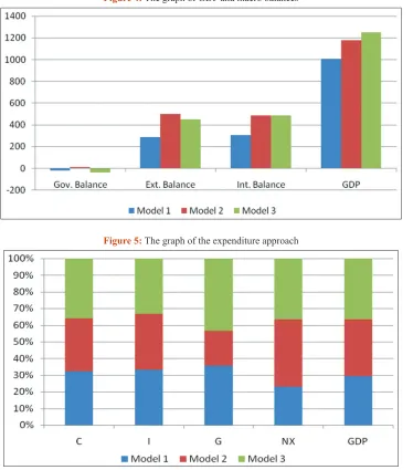
The economy is illustrated under experimental models as in Table 5 and 6. The simulation result shows how institutions interact in the markets. Table 5 shows relationship between expenditure (government, households) and income (customers,

firms). Table 6 illustrates GDP and macro balances. Internal balance indicates relationship between saving (customer saving and firm profit) and investment (capital investment and capital depreciation). External balance indicates trade balance between export and import. Government balance indicates relationship between government revenue (tax and subsidy) and government expenditure. Sustainability analysis is concerned on changes in macro balances and sector structure, and their effects to GDP growth as in Figure 4.

The expenditure approach measure GDP by using data on personal expenditure, capital investment, government expenditure, and net export. GDP using in the expenditure approach is the sum of personal expenditure (C), capital investment (I), government expenditure (G), and net export (NX). Table 7 shows the expenditure approach for GDP measurement of the economy.

GDP C I G NX= + + + (33)

Table 6: Results of changes in GDP and macro balances

Models Formula Model 1 Model 2 Model 3

% Agriculture

1

X 35% 30% 25%

% Industry

2

X 30% 35% 35%

% Services

3

X 35% 35% 40%

GDP GDP 1008.57 1176.67 1251.25

Government Balance

1 1

= =

− ×

∑ ∑

m j m j Gj

j j

T P Q -19.16 13.56 -36.77

External Balance

1

=

× ×

∑

m j NXj j

j

P Q EX 286.00 500.00 449.85

Internal Balance

1 1 1

= = =

× + × ×

∑

m j Gj

∑

m j NXj j

∑

m j

j j j

P Q P Q EX - T 305.16 486.44 486.62

Sources: These above formulas are adapted from Trinh (2017b)

Figure 4: The graph of GDP and macro balances

Figure 5: The graph of the expenditure approach

capital depreciation (D), tax and subsidy (T). GDP using the income approach is the sum of personal expenditure (C), capital depreciation (D), total saving (S), tax and subsidy (T). Table 8 shows the expenditure approach for GDP measurement of the economy.

GDP C D S T= + + + (34)

Figure 6: The graph of the income approach

Figure 7: The circular flow of the Model 3

Table 7: The expenditure approach for GDP measurement

Items Symbol Model 1 Model 2 Model 3

Personal expenditure C 598.42 585.23 659.63 Capital investment I 45.00 45.00 45.00 Government

expenditure G 79.16 46.44 96.77 Net export NX 286.00 500.00 449.85 Gross Domestic

Product GDP 1008.57 1176.67 1251.25

Table 8: The income approach for GDP measurement

Items Symbol Model 1 Model 2 Model 3

Capital interest K×WK 406.96 539.02 551.41 Labor wage L×W_L 486.61 373.54 570.27 Firm saving S_F 10.00 159.11 24.57 Capital depreciation D 45.00 45.00 45.00 Tax and subsidy T 60.00 60.00 60.00 Gross Domestic

Product GDP 1008.57 1176.67 1251.25

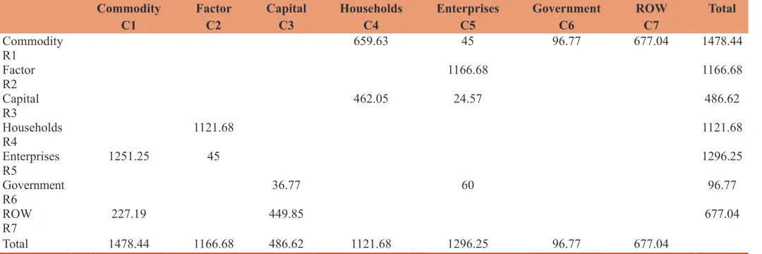
SAM result indicates that total supply is equal to total demand for all markets as in Table 9. Internal balance (П + S_c = 486.62) comes from firm profit (П = 24.57) on the commodity market and customer saving (S_c = 462.05) on the factor markets. Government balance and external balance are adjusted on the financial markets, in which internal balance (486.62) is also equal to subtraction of external balance (449.85) from government balance (-36.77).

Figure 7 illustrates for Model 3. Households receive capital interest and labor wage (K×W_K + L×W_L = 1121.68) from the factor markets, and make personal expenditure (C = 659.63) in the commodity markets. Enterprises make capital investment (I = 45) and get capital depreciation (D = 45), government purchases commodities (G = 96.77), and the rest of the world (ROW) purchases net export (NX = 449.85). Total saving (S = 486.62) includes customer (household) saving (S_C = 462.05) and firm (enterprise) saving (S_F = 24.57). Customer saving (S_C = 462.05) and firm profit (П= 24.57) would lend in the financial market, where government and the rest of the world would borrow to finance their deficits.

5. CONCLUSIONS

This paper provides a conceptual framework with basic principles in general equilibrium modeling for economic policy analysis as a good start to understand the more complex CGE models. The starting point in the CGE modeling is the understanding on the basic structure and key flows of the economy. The basic general equilibrium model is developed with the objective function of GDP under the constraints of market equilibriums and macro balances. Economic policies are proposed from the combinations of macro closures in response to the context of economic policy analysis. The simulation experiment is carried out on the hypothetical economy with target sector structures. The experiment is to analyze changes in economic policy (target sector structure, government balance, external balance, internal balance) on the economic growth and transition.

The paper contributes an insightful understanding on the way of GDP measurement and mechanism of general equilibrium in the economy. However, this paper has some limitations that also suggest for the future researches: (1) econometric techniques are used to estimates parameters in the CGE models; (2) market price system should be explored upon market behaviors in nature; (3) elasticities of substitution and transformation should be considered in the CGE models; and (4) the future researches should expand with multiple sectors with SAM data of the economy.

ACKNOWLEDGEMENT

This research was presented at the Ninth Vietnam Economist Annual Meeting (VEAM 2016) and the 27th _{EBES Conference – Bali (Best} Paper Award). This research was supported by Funds for Science and Technology Development of the University of Danang [project number B2017-ĐN04-06].

REFERENCES

Arrow, K.J., Debreu, G. (1954), Existence of an equilibrium for a competitive economy. Econometrica, 22(3), 265-290.

Baier, K. (1966), What is value? An analysis of the concept. In: Baier, K., Rescher, N., editors. Value and the Future: The Impact of Technology Change on American Values. New York: The Free Express. p33-67. Bentham, J. (1789), An Introduction to the Principles of Morals and

Legislation. Oxford: Clarendon Press.

Dupuit, J. (1844), On the measurement of the utility of public works. International Economic Papers, 2(1952), 83-110.

Grönroos, C. (2011), A service perspective on business relationships: The value creation, interaction and marketing interface. Industrial Marketing Management, 40(2), 240-247.

Grӧnroos, C. (2008), Service logic revisited: Who creates value? And who co-creates? European Business Review, 20(4), 298-314.

Grӧnroos, C., Voima, P. (2012), Making Sense of Value and Value Co-creation in Service Logic. Helsinki, Finland: Hanken School of Economics.

Hosoe, N., Gasawa, K., Hashimoto, H. (2010), Textbook of Computable General Equilibrium Modeling. London: Programming and Simulations Palgrave Macmillan.

Jevons, S.W. (1871), Theory of Political Economy. London: Macmillan. Lofgren, H., Harris, R.L., Robinson, S. (2002), A Standard Computable

General Equilibrium (CGE) Model in GAMS. Washington DC: International Food Policy Research Institute (IFPRI).

Marshall, A. (1890), Principles of Economics. London: Macmillan. Menger, C. (1871), Principles of Economics. Germany: Braumüller. Ricardo, D. (1821), On the Principles of Political Economy and Taxation.

London: John Murray.

Smith, A. (1776), The Wealth of Nations. New York: The Modern Library. Sue Wing, I. (2009), Computable general equilibrium models for the

analysys of energy and climate policies. In: Evans, J., Hunt, L.C., editors. International Handbook on the Economics of Energy. Chettenham: Edward Elgar. p332-366.

Table 9: SAM results for Model 3

Commodity

C1 Factor C2 Capital C3 Households C4 Enterprises C5 Government C6 ROW C7 Total Commodity

R1 659.63 45 96.77 677.04 1478.44

Factor

R2 1166.68 1166.68

Capital

R3 462.05 24.57 486.62

Households

R4 1121.68 1121.68

Enterprises

R5 1251.25 45 1296.25

Government

R6 36.77 60 96.77

ROW

R7 227.19 449.85 677.04

Trinh, T.H. (2014), A new approach to market equilibrium. International Journal of Economic Research, 11(3), 569-587.

Trinh, T.H. (2017a), A primer on GDP and economic growth. International Journal of Economic Research, 14(5), 13-24.

Trinh, T.H. (2017b), Value balance and general equilibrium model. International Journal of Economics of Financial Issues, 7(2), 485-491. Trinh, T.H. (2018), Towards a paradigm on the value. Cogent Economics

and Finance, 6(1), 1429094.

Trinh, T.H., Kachitvichyanukul, V., Khang, D.B. (2014), The co-production approach to service: A theoretical background. Journal

of the Operational Research Society, 65(2), 161-168.

Vargo, S.L., Lusch, R.F. (2004), Evolving to a new dominant logic for marketing. Journal of Marketing, 68(1), 1-17.

Walras, L. (1874), Elements of Pure Economics. London: George Allen and Unwin.

Wikström, S. (1996), The customer as co-producer. European Journal of Marketing, 30(4), 6-19.