Application of PFC
3D
to simulate a planetary ball mill
L. Guzman
1, Y. Chen
1*, S. Potter
2, M.R. Khan
1(1.Department of Biosystems Engineering, University of Manitoba, Winnipeg, MB, Canada;
2.Composites Innovation Centre, Winnipeg, MB, Canada)
Abstract: Planetary ball mill is a versatile machine which has been used for grinding different types of materials for size reduction and lately for hemp decortication. PFC3D, software employing the discrete element method (DEM), was used to simulate the power and energy requirement of grinding hemp for fibre using a planetary ball mill. The simulation was facilitated through a series of hemp grinding tests using the planetary ball mill to examine the power draw of the mill. The test results identified that grinding speed had a significant effect on the power draw of the mill. The power draw data were used to calibrate the discrete element parameters for different grinding speeds. Using the calibrated parameters, one was able to predict the kinetic energy and friction power loss of the ball mill. The average value of kinetic energy predicted, for grind ing speeds of 200 – 500 r/min, ranged between 0.01 and 0.07 J per grinding ball. The prediction showed that frictional power losses dispersed approximately 10% of the total power requirement of the ball mill. Overall, the simulation using PFC3Dimproved understanding about the dynamics of the grinding balls within a planetary ball mill as well as the energy available for transfer in collisions between the grinding balls and hemp material.
Keywords: PFC3D, Discrete element model (DEM), hemp, planetary ball mill, power, energy, kinetic, friction
Citation: Guzman,L.,Y. Chen, S. Potter, and M.R. Khan. 2015. Application of PFC3D to simulate a planetary ball mill. Agric Eng Int: CIGR Journal, 17(4):235-246.
1 Introduction
1Planetary ball mills are well suited for
laboratory-scale processing of materials in diverse
industries (Rosenkranz et al., 2011). A future objective of
industry is to develop large-scale units for industrial
manufacturing purposes. Overall, ball mills were able to
defibrillate fibrous materials as well as improve fibre
fineness by applying impact and shear forces (Prasad et
al., 2005). Previous studies by our research group have
demonstrated promising potential of ball milling for
hemp (Cannabis sativa Linnaeus) decortication (Baker et
al., 2010) and for hemp fibre refining (Khan et al., 2009).
Decortication is a mechanical process of extracting raw
hemp fibres, which is an energy intensive process
because hemp plants possess a high percentage of
cellulose and lignin. Commonly used decortication
Received date: 2014-07-28 Accepted date:2015-09-20 *Corresponding author: Ying Chen, Department of Biosystems Engineering, University of Manitoba, Winnipeg, Manitoba R3T 5V6, Canada. Tel.: 1 204 474 6292. fax: 1 204 474 7512. E-mail: [email protected].
equipment for hemp includes hammer mills, cutter heads,
and roll crushers. Each piece of decortication equipment
operates under different principles involving the
application of forces to the hemp stalk and obtaining the
fibre (Fürll and Hempel, 2000; Gratton and Chen, 2004).
All of these machines have multiple rotating parts, such
as shafts and bearings, which are in contact with hemp,
causing hemp fibre wrapping around these rotating parts
(Dietz, 1999; Hobson et al., 2001). Hence, an operational
limitation of these machines is the need for frequent stops
to remove wrapped fibres and prevent any further damage
to the machines. Ball mills are alternative machines for
hemp decortications. The main advantage of using ball
mills is that fibres are not in contact with any rotating
machine parts. Hence, fibre wrapping problems are no
longer a concern.
The focus of this study was on the dynamic
behaviours of a planetary ball mill in the context of hemp
decortication. The working principle of a planetary ball
mill is based on the movement of a grinding bowl, filled
superimposed rotational movements. The difference in
speeds between the grinding balls and grinding bowl
produces an interaction between frictional and impact
forces, which releases high dynamic energy. Inside a
planetary ball mill, multiple collision events transfer
impact energy from the grinding balls to the material (e.g.
hemp sample) (Lynch and Chester, 2005). The energy
available for all collision events is provided by the
movement of the grinding bowl, which is driven by an
electric motor. Hence, there is a direct relationship
between the total power draw of the mill and impact
energy of the grinding balls. To design efficient and
effective ball mills, research is required to provide
information about energy transfer mechanisms acting
within the planetary ball mill. The information includes
power requirement, kinetic energy, and frictional power
loses. Since direct observation by means of on-line
sensors is impractical, and dynamic behaviours of
grounding balls and their interactions with material are
very complex and difficult to measure, the best option is
numerical simulation (Mishra, 2003a).
One of the most effective methods of simulating
behaviours of individual particles (e.g. grinding balls) is
using the discrete element method (DEM). The DEM is a
time-stepping algorithm that requires three main elements:
the repeated application of Newton's second law of
motion to each particle (grinding ball) inside the
considered system (grinding bowl); a force–displacement
law to each contact; and a constant update of particle
(grinding ball) and wall (grinding bowl) positions. The
DEM has been successful at approximating ball milling
internal behaviour and motion patterns. Radziszewski
(2002) modelled media wear mechanisms of a mill using
the DEM. The model was calibrated and validated with
lab tests of ore-metal. That study also listed other studies
using the DEM to describe the dynamics inside mills.
Cleary and Hoyer (2000) simulated the charge motion of
a centrifugal mill in an application of grinding quartz
using steel balls. The most significant affecting factor
reported was the mill operational speed (rpm).Planetary
ball mills have been also modelled using the DEM. The
motion of steel balls was affected by the type of feed and
the friction of the media (Rosenkranz et al., 2011). Sato et
al. (2010) tried to relate wear to the impact energy of steel
balls of a planetary ball mill. They found that wear rate
increased with the increase of mill operational speed, ball
diameter, and ball-filling ratio.
One of common DEM softwars, Particle Flow Code
in Three Dimension (PFC3D), has several features which
are suitable for simulation of a planetary ball mill. Using
PFC3D, moving balls in a mill can be described with
translational and rotational motions. It also takes
frictional force into consideration between the contacts of
balls. Several dynamic attributes of balls, such as kinetic
energy and friction energy, can be monitored while the
ball mill is in operation.
In summary, little work has been done on planetary
mills with non-steel material as media and using PFC3Das
the modelling tool. The objectives of this study were to: 1)
apply PFC3Dto simulate a planetary ball mill; 2) calibrate
the PFC3D parameters with measurements from hemp
decortication; and 3) predict dynamic behaviours of
grinding balls inside the mill.
2 Methodology
2.1 Description of the planetary ball mill
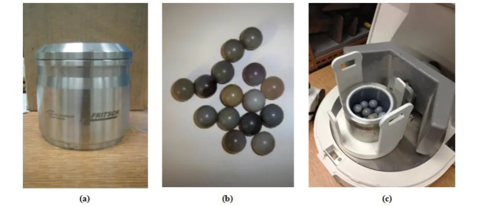
A planetary ball mill (Fritsch Pulverisette 6 classic
line, Idar-Oberstein, Germany) was used in this study.
The machine consisted of a cylindrical grinding bowl
with an inner diameter of 74.5 mm and a height of 86.7
mm (Figure 1a). The effective volume of the bowl was
250 ml. The grinding media consisted of 15 spherical
balls (Figure 1b) with a 20-mm diameter. The balls were
made of agate with a density of 2650 kg/m3. The inside of
the bowl had an agate liner. Thus, the interaction between
the bowl and balls was agate to agate. The bowl was fixed
on a support disc (Figure 1c) and the distance between the
axle of the bowl and the axle of the support disc was 62.5
mm. The mill was powered by a 1.1 kW electric motor.
also rotated with the support disc in the opposite direction.
The relative speed ratio of the bowl to the supporting disc
was 1.82. For every full rotation of the disc, the grinding
bowl rotates 1.82 revolutions about its own centre in the
opposite direction.
2.2 Simulation
2.2.1 Model of the planetary ball mill
All the dimensions and properties of the ball mill
within the model were equivalent to those of the
aforementioned planetary ball mill. The PFC3D version
4.00 was used to develop the model of the planetary ball
mill. The main component of the model was the assembly
of grinding balls which were represented by spherical
particles (Figure 2). The constitutive laws for the contact
between particles were described by the Stiffness and Slip
Models implemented in PFC3D. These Models provide an
elastic relation between the contact force and the
displacement of particles, and allow two contacting
particles to slip relative to each other, introducing a
friction force between the particles.Rosenkranz et al.
(2011) reported some significant effects of rolling friction
of particle, whereas Cleary and Hoyer (2000) reported
mixed results about the effects of rolling friction,
depending on the mill fill level. It is advised that rolling
friction was not considered in the model of this study.
Fifteen balls were enclosed inside a bowl which was
constructed using a cylindrical wall as the body of the
bowl and two flat square walls as the bottom and top
covers of the bowl. The largest disc functions as the Figure 1 Principal components of a planetary ball mill: (a) grinding bowl; (b) grinding balls; (c) relative
position of the grinding bowl on the supporting disc
supporting disc. The medium-sized disc is the grinding
bowl support, and it was used to ensure that the distance
between the centre of the bowl and the centre of the
support disc was constant at all times. At the
commencement of the simulation, it was assumed that the
grinding balls were settled at the bottom of the bowl. The
grinding balls were generated inside the bowl and the
model was operated in a stationary state to allow the balls
to settle at the bottom of the bowl due to the force of
gravity. Before running the simulations, a detailed
examination of the location of the grinding bowl was
performed to ensure the right relative motion and position
between the grinding bowl and supporting disc. This was
done through monitoring the position of the grinding
bowl with a tracking particle following the same motion
pattern as the grinding bowl support. The tracking
particle was located in the centre of the grinding bowl and
it was positioned in such a way that it would not interact
with the grinding balls inside the grinding bowl.
2.2.2 Motion generation
Figure 3 shows a simplified diagram of the relative
motion of the grinding bowl with respect to the
supporting disc. The rotational speed of the supporting
disc was an adjustable variable in the simulation and was
assigned values corresponding to the tests. As described
earlier, the angular velocity of the grinding bowl about its
own centre was given by Equation (1):
Figure 3 Motion diagram of the planetary ball mill (R =
distance from the centre of the supporting disc to the
centre of the grinding bowl; r = radius of grinding bowl;
ω = angular velocity of supporting disc; β = angular
velocity of the grinding bowl)
β =-1.82 ω (1)
where
β = angular velocity of the grinding bowl, rad/s;
ω = constant angular velocity of the supporting disc,
rad/s.
The motion produced by the supporting disc was
modelled as a function of ω and time. The absolute linear
velocity of the centre of the grinding bowl with respect to
the centre of the supporting disc was given by Equation
(2):
V=Rω (2)
where
V = absolute linear velocity of the centre of the
grinding bowl, m/s;
R = distance from the centre of the grinding bowl to
the centre of the supporting disc, m.
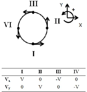
The function for circular displacement of the
grinding bowl about the centre of the supporting disc was
categorized as two-dimensional motion parallel to the
plane of the supporting disc. The function for circular
displacement was obtained by breaking the absolute
linear velocity into two vector components, Vx and Vy.
The magnitude of these vector components was given as
a function of the time required to complete one full
revolution with boundary conditions as illustrated in
Figure 4.
Figure 4 Boundary conditions for vector components of
The Equation (3a) and Equation (3b) for the vector
components of the absolute displacement velocity were
derived as:
( ) (3.a)
( ) (3.b)
where
t1/4= the time required to complete one quarter of a
revolution, s;
t = the total accumulated time of the model, s.
The value of t1/4 was fixed depending on the
magnitude of the rotational speed of the supporting disc.
The variable t started at zero and increased with each time
step in the same units as t1/4. The value of t1/4 was derived
directly from the number of revolutions per minute as
Equation (4):
(4)
where
n = number of revolutions per minute, r/min.
Application of the previously described boundary
conditions produced the desired motion within the model.
The proposed system of equations worked for any
assigned speed, while maintaining the same geometrical
relationships found in the planetary ball mill. Figure 5
shows the displacement velocities of the centre of the
grinding bowl with respect to the centre of the disc.
Simultaneously, the grinding bowl constantly rotated
about its own centre at an angular velocity equivalent to
β.
Figure 5 Change in velocity components over time at 200
r/min
2.2.3 Model parameters
The integration of DE equations required parameters
which describe the contact nature between balls and bowl.
The application of linear contact models was discussed in
the work of Mishra (2003b). The linear model is defined
by the normal and shear stiffness, Kn and Ks, of the two
contacting entities (ball-to-ball and ball-to-wall). Stiffness
had some effects on the internal dynamics of mill (Cleary
and Hoyer, 2000). In this study, this parameter was
determined from the Young’s modulus of the material
(Cundall and Strack, 1982; Chang et al., 2003) using the
following Equation (5) (Itasca, 2012):
̅ (5)
where
Kn= the normal stiffness, N/m;
Rp= the ball radii, m;
E = the apparent young’s modulus, Pa.
The grinding balls and the walls within the model
were assigned contact properties that were equivalent to
Agate stones, with a density of 2650 kg/m3 and a
modulus of elasticity of 70 GPa (Fossen, 2010).
Application of the relationship in Equation (5) resulted in
a normal stiffness, Kn, value of 2.8x10 9
N/m. The shear
stiffness, Ks, was assigned the same value as the normal
stiffness as in many other studies (e.g. McDowell and
Harireche, 2002; Asaf et al., 2007). A low value was
taken for the friction coefficient of the balls, considering
their polished surfaces. The values of all model
parameters are summarized in Table 1.
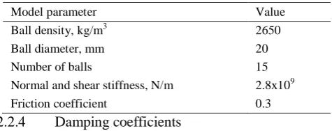
Table 1 DEM parameters applied to simulation
Model parameter Value
Ball density, kg/m3 2650
Ball diameter, mm 20
Number of balls 15
Normal and shear stiffness, N/m 2.8x10⁹
Friction coefficient 0.3
2.2.4 Damping coefficients
In DE models, energy supplied to the particles needs
dissipation with damping mechanisms to arrive to a
steady state solution (Itasca, 2012). The PFC3D code is
able to dissipate kinetic energy with two types of
applies a damping force to each ball, while viscous
damping applies the damping force to each contact
(ball-ball or ball-wall).Viscous damping has two damping
components, normal (Vdn) and shear (Vds). As a general
rule of thumb, local damping is most appropriate for
compact assemblies while viscous damping is preferred
for situations involving free flight of particles or impacts
between particles. The planetary ball mill was subject to
both scenarios because it behaved as a compact assembly
at low grinding speeds but particles took flight and
collided at higher grinding speeds. The combination of
these two types of damping would provide the most
accurate physical representation of the ball assembly, and
they were calibrated.
2.3 Calibration of the damping coefficients
The damping coefficients (Ld, Vdn, and Vds) were
calibrated using measurements of the ball mill power
from tests. The tests and calibration method are described
in the following sections.
2.3.1 Measurements of power requirement of the ball
mill
To calibrate the model, data on the power
requirement of the mill were collected in tests of hemp
grinding. Hemp samples (variety: USO 31) were stored to
air dry to a moisture content of approximately 10%.
Before being ground, hemp samples were cut into 40-mm
stalk segments so that they could fit into the grinding
bowl. The grinding bowl was filled with an
approximately six grams based on the ball mill feeding
capacity. The magnitude of the power requirement for
grinding was expected to be affected mainly by the mill
speed. A range of different grinding speeds was selected:
200, 300, 400, and 500 r/min according to the operational
specifications of the mill. Power requirement may also
change over time while a hemp sample is being ground,
as the hemp particle size changes over time. Therefore,
grind tests were performed for three grinding durations: 3,
5, and 8 min at each grinding speed. The power draw in
the grinding process was measured with a watt-hour
meter directly connected to the ball mill. Before each test,
the power consumption without hemp was recorded for 5
min. Comparison of the average power draws between
the conditions with and without samples served as a
means to determine the net power draw for hemp
grinding.
2.3.2 Model prediction of power
The ball mill model was run at the default time step
of PFC3Dto predict the power required for moving the
grinding balls inside the bowl. This power is equivalent to
the total accumulated work of the walls (i.e. the inside of
the grinding bowl) on the assembly of balls. The PFC3D is
able to monitor this work which is defined as Equation (6)
(Itasca, 2012):
∑ (6)
where
Ew = the total accumulated work of the wall;
Nw = the number of walls (one cylindrical wall and
two flat walls in this case);
Fi and Mi = the resultant force and moment acting on
the walls, respectively;
Ui and θi = the applied displacement and rotation,
respectively.
Under the assumption that all the energy provided to
the systems originated from this source, the power was
calculated through the magnitude of Ew divided by the
total accumulated time. The magnitude of Ew was positive
or negative, with the convention that work of the walls on
the particles is positive. Calibrations of damping
coefficients were performed through comparisons of the
powers measured and simulated. The calibrated damping
confidents were those values which resulted in the best
match between measurements and simulations.
3 Results and discussion
3.1 Tests and calibration results
3.1.1 Measured power requirement
The difference between power draw measurements
with and without hemp samples, was used to calculate the
net power draw required to grind the samples. The
W, which was only approximately 1%-5% of the total
power draw measured. A paired t-test, with a 5% level of
significance, showed that the differences in draw power
were insignificant between the conditions with and
without hemp sample in the bowl. In addition, the net
power data had no particular trends, in terms of effects of
grinding speed and duration. Although the hemp sample
occupied a significant volume inside the grinding bowl, it
did not affect the power required to operate the mill. A
possible explanation is that the hemp sample possessed a
relatively small mass of grinding balls. The tests
demonstrated that grinding media (balls) and its dynamics
were the major factors affecting the power draw of ball
milling.
Given the insignificant differences between tests
with hemp and without hemp, the total power data pooled
from the tests with hemp and without hemp were used to
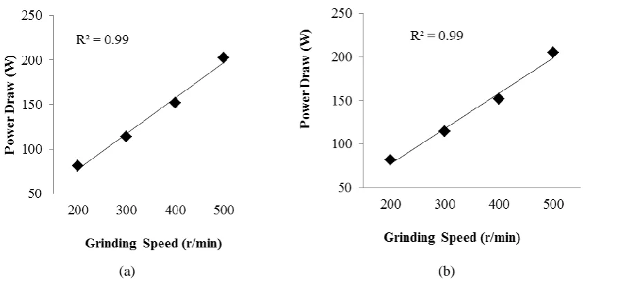
examine effects of grinding speed. The results showed
that milling at larger rotational speeds required increasing
amounts of input power (Figure 6a and Figure 6b). The
relationship between the power draw and rotational speed
could be described as a linear relationship with a
coefficient of determination of 0.99. The results showed
that the power draw did not vary with the grinding
duration (data not shown). For example, at 400 r/min,
power draw was determined as 151 ± 6, 152 ± 7, and 153
± 9 W for 3, 5, and 8 min respectively.
3.1.2 Effects of damping coefficients on the power
requirement
Simulations demonstrated that as the damping
coefficients were adjusted, dissipation of more energy
due to damping would cause lower magnitudes of the
power predicted by the model. An example of this type of
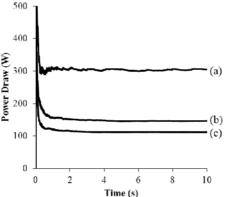
behaviour is present in Figure 7, in which every
parameter remains constant with the exception of two
damping coefficients. It was clear that the damping
coefficients significantly affect the model outputs both
over time and in magnitude. Dynamic behaviours of the
ball assembly were very sensitive to the input viscous
damping coefficients.
(a) (b)
Figure 6 Variations of power draw of the planetary ball mill with grinding speed: (a) with hemp sample; (b)
Figure 7 Effect of damping coefficient on power draw at
400 rpm; Ld=0.4: (a) Vdn= Vds=0; (b) Vdn= Vds=0.3; (c)
Vdn=Vds=0.6 (Ld=local damping coefficient; Vdn
andVds=viscous normal and shear damping coefficients
respectively)
3.1.3 Power comparisons between simulations and
measurements
The test results demonstrated that the addition of
hemp material and grinding duration did not significantly
affect the power draw. This information provided the
base for simplifying the model without involving hemp
particles in the model, which allowed for a representative
simulation of the planetary ball mill. The measured power
draw was the total energy introduced into the planetary
ball mill from the electricity source. The difference
between the measured power draw and the simulated
power was that the measured power included the
mechanical loss in the process of transmitting electricity
energy to the ball assembly. The mechanical loss was
assumed as 10% of the total power draw (Wills, 1979).
Thus, the values of the measured power draw were
reduced by 10% before being compared with the powers
predicted by the model.
The power was simulated for multiple combinations
of Ld, Vdn, and Vds at different grinding speeds (200, 300,
400, and 500 r/min). The results showed that changes in
Ld had little influence in power after the grinding balls
engaged in free flight, whereas changes in Vdn and Vds
had significant effects in the power. For simplicity, values
of Ld were kept constant for the different grinding speeds
and values of Vdn and Vds were kept the same for each
speed. Results demonstrated that there was not a single
value of Vdn and Vds that would accurately approximate
the power draws measured for all grinding speeds. For
example, with a value of Vdn and Vds, the predicted value
of power for the 200 rpm would be comparable to the
measurements, but that for the 300 rpm would have a
relative error of over 40% when compared to the
measurement. These results indicated that the Vdn and Vds
were grinding speed dependent. Hence, a specific value
of Vdn and Vds was required to be calibrated for each
grinding speed.
In calibrating the damping coefficients for different
grinding speeds, it was found that a constant value (0.4)
was an adequate Ld for all speeds. With this constant Ld,
the input Vdn and Vds were being adjusted during the
simulation until the predicted power best matching the
measured one. The best match was considered as the least
relative error between the predicted and measured powers.
Table 2 lists the calibrated results and the least relative
errors obtained. The calibrated values of Vdn and Vds were
increased as the grinding speed increased, which
represented the slowing down of grinding balls. The
average relative errors for the speeds of 200, 300, and 400
rpm were all below 10%, which indicated that the model
was able to adequately approximate the power. However,
3.2 Simulations of dynamic behaviours of the
planetary ball mill
The calibrated model was used to simulate the
kinetic energy and friction loss of the ball assembly. To
better understand these, motion patterns of the balls were
also visually examined. All simulations were performed
under different grinding speeds using the calibrated
damping coefficients listed in Table 2.
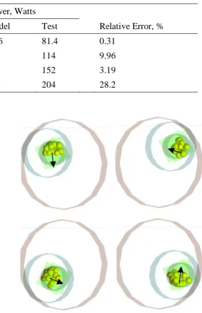
3.2.1 Motion pattern of the balls
Figure 8 provides an example of monitoring
grinding balls to determine their locations after one full
revolution. The grinding balls followed a cascading type
of motion for the proposed range of grinding speeds. The
grinding balls were ―flying‖ towards the opposite end of
the cylinder wall. Movement of the grinding balls within
the ball mill led to collisions, which became the main
mechanism transferring energy from the grinding balls to
the hemp sample.
Figure 8 Screenshot of grinding ball motion pattern after
one full revolution of the grinding bowl
The monitoring of the velocity distribution within
grinding balls helps supplement grinding ball position
information. The proposed model was able to record the
translational velocity distribution at different grinding
speeds. The velocity distribution (Figure 9) indicates that
grinding balls adjacent to the bowl wall have a different
translational velocity than those closer to the centre of the
grinding bowl. The differences in translational velocities
were in the order of 0.5 m/s, which support the argument
for calculating the average kinetic energy of each ball as
the average kinetic energy within the model.
Table 2Calibrated damping coefficients for different mill speeds
Speed, r/min Damping Coefficient Power, Watts
Ld Vdn Vds Model Test Relative Error, %
200 0.4 0 0 81.6 81.4 0.31
300 0.4 0.3 0.3 102 114 9.96
400 0.4 0.6 0.6 147 152 3.19
500 0.4 1.2 1.2 264 204 28.2
Through enhanced understanding of motion patterns,
the DEM enabled future study of design factors such as
the operational grinding speed, sizes of the grinding balls
and bowl, friction coefficients, and the ratio of material to
bowl volume. These design factors have a direct effect in
the effectiveness and location of the grinding areas where
high impact forces decorticate the hemp sample.
3.2.2 Kinetic energy of the balls
Previous studies (Abdellaoui and Gaffet, 1995;
Magini et al., 1996; Iasonna and Magini, 1996)
determined collision energy by linking it directly to the
kinetic energy of each individual grinding ball. The
collision energy in the planetary ball mill was assumed
equivalent to the total kinetic energy of the balls’ motion.
The proposed model was able to determine the total
kinetic energy of all particles accounting for both
translational and rotational motion as Equation (7) (Itasca,
2012):
∑ (7)
where
Ek = total kinetic energy;
Nb, mi, Ii, Vi and ωi= the number of balls, inertial
mass, inertia tensor, and translational and rotational
velocities of ball i, respectively.
The average kinetic energy provides information
about the amount of energy available for transfer from the
grinding balls into the hemp stems. Average kinetic
energy was approximated for each ball from the division
of the total kinetic energy by the number of grinding balls
present in the model. The average magnitude of the
modelled kinetic energy, for each given grinding speed,
consisted of slight diversions in magnitude about an
average value. An example of the kinetic energy output
from the model is shown in Figure 10, which includes the
range of values of the total kinetic energy including all
grinding balls at a grinding speed of 200 r/min for 10 s.
Figure 10 Simulated total kinetic energy predicted by the
model for the 200 r/min grinding speed
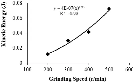
Results of the average kinetic energy per ball
obtained from the model were plotted in Figure 11. The
order of magnitude of the predicted kinetic energy was in
accordance with studies performed by Magini et al.
(1996), who established that the collision energy of
individual balls was in the order of 10-2 J per collision.
The best fit curve of the data was found to follow a power
relation with a coefficient of determination of 0.98. The
predicted kinetic energy provided information about
energy transferred from the grinding balls into the hemp
sample during milling.
Figure 11 Simulated average kinetic energy per ball at
different grinding speeds
3.2.3 Frictional power losses
A portion of the power introduced into the system
model, the total accumulated frictional energy loses was
defined (Itasca, 2012) as Equation (8):
∑ (8)
where
Ef = total accumulated frictional energy loss;
Nc = the number of contacts;
Fis and ∆Uis= the average shear force and the
increment of slip displacement respectively.
The parameter Ef represents the magnitude of the
total accumulated energy dissipated through frictional
sliding at all contacts. The total friction power losses
were calculated from dividing the total energy dissipated
through friction with the total accumulated time. Figure
12 shows a typical curve of friction loss over time.
Figure 12 Simulated friction power losses at 200 r/min
The magnitude of the frictional power losses
increased at larger grinding speeds (Figure 13). However,
frictional power losses represented only a small
percentage of the total power. The energy dispersed
through friction at 200, 300, 400, and 500 rpm accounted
for 5.7%, 11%, 11%, and 13% of the total power
respectively. In average, it was determined that
approximately 10% of power was dispersed as frictional
energy. After frictional losses, the remaining applied
energy is mostly in the form of kinetic energy driving
high energy impacts during the milling process.
Figure 13 Friction power losses at different grinding
speeds
Although further experiments are required to
determine the applicability of current model parameters
to different types of milling arrangements, the PFC3D
could potentially evaluate the effect of various conditions
through changing the variables such as grinding media,
grinding speed, and mill dimension. Hence, the proposed
model improves its capacity to recreate and understand
the dynamics inside a planetary ball mill.
4 Conclusions
The planetary ball mill was successfully modelled
using a PFC3D with appropriate geometrical relationship
of the motion in the grinding bowl. Test results showed
that the energy consumption of milling hemp was
attributable mainly to the grinding media, not the hemp
being ground.Based on the test results, the model was
simplified without considering effects of hemp material.It
was found that viscous damping coefficients were the
most crucial model parameters in this application, and
they are grinding speed dependent. The calibrated model
for different mill speeds is suitable for mill speeds lower
than 400 r/min. The model is able to simulate the kinetic
energy and frictional power losses of the ball assembly of
the mill. The simulations revealed that both the kinetic
energy and friction power losses had a power relationship
with the grinding speed. Further experiments and research
are required to evaluate the applicability of the results for
Acknowledgements
The research was supported by Natural Sciences and
Engineering Research Council of Canada (NSERC) and
Mathematics of Information Technology and Complex
Systems, Canada (MITACS).
References
Abdellaoui, M., and E. Gaffet.1995. The physics of mechanical alloying in a planetary ball mill: mathematical treatment.ActaMetallurgicaetMaterialia,
43(3):1087-1098.
Asaf, Z., D. Rubinstein, and I. Shmulevich.2007. Determination of discrete element model parameters required for soil tillage.Soil & Tillage Research, 92(2): 227–242.
Baker, M.L., Y. Chen, C. Lague, H. Landry, Q. Peng, W. Zhong, and J. Wang. 2010. Hemp fibre decortications using a planetary ball mill. Canadian Biosystems Engineering, 52(2):2.7-2.15.
Chang, C. S., C. L. Liao, and Q. Shi.2003. Elastic granular materials modeled as first order strain gradient continua.
International Journal of Solids and Structures, 40: 5565–5582.
Cleary P., and D. Hoyer. 2000. Centrifugal mill charge motion and power draw: comparison of DEM predictions with experiment. International Journal of Mineral Processing, 59:131-148.
Cundall, P. A., and O. D. L. Strack.1982. Modeling of microscopic mechanics in granular material. In: J. T. Jenkins, & M. Satake (Eds.), Mechanics of Granular Materials: New Models and Constitutive Relations (pp. 113–149). Amsterdam: Elsevier.
Dietz, J. 1999. Hemp growing pains. The Furrow,104:16-18. Fossen, H.2010. Structural Geology. 1sted. New York, USA:
Cambridge University Press.
Fürll, C., and H. Hempel.2000. Effective processing of bastfiber plants and mechanical properties of the fibers. ASABE Paper No. 046091. St. Joseph, Mich.: ASABE.
Gratton, J. L., and Y. Chen.2004. Development of a field-going unit to separate fibre from hemp (Cannabis sativa) stalk.
Applied Engineering in Agriculture, 20(2):139-145. Hobson, R. N., D. G. Hepworth, and D. M. Bruce.2001. Quality of
fibre separated from unretted hemp stems by decortication.Journal of Agricultural Engineering Research, 78(2): 153-158.
Iasonna, A., and M. Magini.1996. Power measurements during mechanical milling. An experimental way to investigate the energy transfer phenomena.
ActaMetallurgicaetMaterialia, 44(3):1109-1117. Itasca.2012.Particle Flow Code in 3 Dimensions (PFC3D), Theory
and Background. Minneapolis, Minnesota, USA: Itasca consulting group, Inc.
Khan, M. R., Y. Chen, O. Wang, and J. Raghavan.2009. Fineness of hemp (Cannabis Sativa L.) fiber bundle after post-decortication processing using a planetary ball mill.
Applied Engineering in Agriculture, 25(6):827-834. Lynch, A., and R. Chester. 2005. The History of grinding. Littleton,
Colorado, USA: Society for Mining, Metallurgy and Exploration Inc.
Magini, M., A. Iasonna, and F. Padella.1996. Ball milling: an experimental support to the energy transfer evaluated by the collision model. ScriptaMaterialia, 34(1):13-19. McDowell, G.R., and O. Harireche.2002. Discrete element
modelling of yielding and normal compression of sand.
Geotechnique, 52(4): 299–304.
Mishra, B. K. 2003a. A review of computer simulation of tumbling mills by the discrete element method: part I—contact mechanics. International Journal of Mineral Processing, 71:73-93.
Mishra, B. K. 2003b. A review of computer simulation of tumbling mills by the discrete element method: part II - practical applications. International Journal of Mineral Processing,71:95-112.
Prasad, B. M., M. M. Sain, and D. N. Roy. 2005. Properties of ball milled thermally treated hemp fibers in an inert atmosphere for potential composite reinforcement.
Journal of Material Science, 40(16):4271-4278.
Radziszewski, P. 2002. Exploring total media wear. Mineral Engineering, 15: 1073-1087.
Rosenkranz, S., S. Breitung-Faes, and A. Kwade.2011. Experimental investigations and modelling of the ball motion in planetary ball mills.Powder Technology, 212:224-230.
Sato, A., J. Kano, and F. Saito. 2010. Analysis of abrasion mechanism of grinding media in a planetary mill with DEM simulation. Advanced Powder Technology, 21:212-216.