The Low Beta Anomaly and Estimation Interval
Brandon K. Renfro1 1
Fred Hale School of Business, East Texas Baptist University, Marshall TX, USA
Correspondence: Brandon K. Renfro, Fred Hale School of Business, East Texas Baptist University, Marshall TX, USA. E-mail: [email protected]
Received: January 30, 2019 Accepted: February 14, 2019 Online Published: February 18, 2019
doi:10.5430/afr.v8n1p203 URL: https://doi.org/10.5430/afr.v8n1p203
Abstract
The purpose of this study was to assess the nature of the relationship between equity beta, and post-estimation return. Specifically, this study sought to address the validity and persistence of the low-beta anomaly across multiple beta estimation intervals. Within the twenty-year sample period from January of 1994 to December of 2013 this research covered ten different beta estimation intervals to determine whether a statistically significant and theoretically consistent relationship existed between equity beta and post-estimation realized return. This research provided two basic conclusions: First, the low-beta anomaly is not robust across multiple beta estimation intervals. Second, with any test of the relationship between beta and return the choice of beta estimation interval matters. Different estimation intervals sometimes provide contradictory empirical results for the same period.
Keywords: low-beta anomaly, capital asset pricing model
1. Introduction
Investment selection and the assessment of risk are important concepts to finance academics, investment professionals, and the investing public. The Capital Asset Pricing Model has long been the gold-standard theoretical tool for determining asset prices in academic research as well as for industry professionals in security markets (Shefrin, 2001)(Clarke, De Silva, & Thorley, 2006).
The core tenet of the Capital Asset Pricing Model is that a security’s return is a function of its exposure to market risk, with expected return increasing as the risk of the security increases. In the Capital Asset Pricing Model, risk is quantified by the measure of beta (Hagin, 1979). A large body of research has been created which incorporates, tests, or extends the CAPM-theorized relationship between beta and return. Some of these tests claim to support, while others claim to discredit, the CAPM. As discredit to the CAPM, a number of published tests suggest that the relationship between beta and return is in fact, inverse. This classification of the beta/return relationship is called the “low-beta anomaly” because of its contrast to the traditional theory as presented in the CAPM.
Beta is measured as the covariance of a security’s return and a given index, divided by the variance of the same index. Commonly, five years of the covariance of monthly returns is used, although this is not a necessity and any covariance and return interval can be used. Although this estimation interval is used extensively in research which supports the low-beta anomaly, there is very little, if any, justification for the selection of this estimation interval over the choice of other estimation intervals.
An important concept for investors and investment practitioners is whether the security market line of the Capital Asset Pricing Model can be applied to real investment decisions in a useful manner.
A number of researchers have addressed this issue by empirically testing the relationship of beta and realized return for individual securities with a majority of research supporting a positive relationship (Baker et al., 2011; Black, Jensen, & Scholes, 1972; Fama & French, 1992; Fama & MacBeth, 1973; Kothari, Shanken, & Sloan, 1995; Sharpe & Cooper, 1972). The predominantly supported view is thus that the relationship between beta and expected return is direct and linear, and is the way it is commonly presented in academic textbooks and classrooms.
true nature of the relationship, and the identification of an appropriate estimation interval, has significant impact on the proper application of beta estimates in making capital allocation decisions.
2. Literature Review
A minority of these empirical tests do not support a strong positive relationship between beta and equity return as predicted by the Capital Asset Pricing Model. Studies mentioned in Blitz et. al. (2014) that have empirically tested the theory of the CAPM suggest a flat or even inverse relationship between beta and realized return. This relationship is known in the academic literature and to practitioners as the “low-beta anomaly”. The low-beta anomaly and theories of its causes are widely discussed in the literature on behavioral finance (Baker et al., 2014; Baker et al., 2011; Blitz et al., 2014).
In order to construct a test of the relationship between beta and equity return it is necessary to first estimate a value for beta, since future beta cannot be known. The most common method of estimating future beta is to use historical return data. (Gregory-Allen et al., 1994; Groenewold & Fraser, 2000). There is also a strong practical appeal to estimating beta in this manner in that the data is readily available from a number of sources, all you need is historical returns for a given security and the benchmark index, and the process does not require overly technical procedures – much like the straightforward intuitive appeal of the CAPM itself.
Two important areas to consider when estimating beta are the stability of beta estimates and the estimation interval used to construct beta estimates. These considerations are critical because beta values may vary based on these factors, which in turn may affect any empirical findings regarding the relationship between beta and return (Groenwold & Fraser, 2000).
Beta stability, referred to as stationarity in such early papers as Alexander & Chervany (1980),Blume (1971), Gooding & O’Malley (1977), and Theobald (1981), is the degree to which beta values remain unchanged through a time series. This is a critical issue to the discussion of the CAPM in this study in that as the value of beta changes, the expected return on a given security will subsequently change (Sharpe, 1964).
Blume (1971) tested the stability of beta for securities and portfolios from July 1926 to June 1968 on portfolios consisting of 1, 2, 4, 7, 10, 20, 35, 50, 75, and 100 securities. Blume divided the sample period into six different seven-year periods. For each period, he calculated beta values for individual securities and grouped the securities into random portfolios containing the number of securities as outlined above. He then compared correlation of individual beta and equal-weight (average) beta of each portfolio to the same measure in the next seven year period. Blume found that the correlations ranged from a low of .59 to a high of 1.00, gradually increasing as the number of securities in the portfolio increased.
His conclusion was that beta values for individual securities were largely unstable but that beta values for portfolios were more stable, and that stability increased as more securities are added to the portfolio (Blume, 1971). Alexander and Chervany (1980) note the importance of accurately measuring beta coefficients in relation to the stability of beta. They conclude that groupings of ten of more securities increase the stability of beta for a portfolio. Abdymomunov and Morley (2011), Bos and Newbold (1984), Groenewold and Fraser ( 2000), Fabozzi and Francis (1978), Ohlson and Rosenberg (1982), and McEnally and Upton (1979) have confirmed these results and it is widely accepted that beta is indeed unstable and time-varying. This fact serves as one of the central tenets of this research.
The beta estimation interval refers to the length of time used for purposes of measuring beta. Beta is found by
Equation 1 where R is return on a security and M is return on the market:
β = COV(R,M)/VAR(M) (1)
What is not designated in the formula is the time interval used to calculate covariance, nor the interval for measuring returns. This leaves open the specific method of calculation which requires two choices to be made.
First, the return interval needs to be identified. Commonly used return intervals correspond to basic calendar intervals such as a day, week, month, quarter, year, etc (Groenewold & Fraser, 2000). Second, the period over which covariance between the security and market return will be calculated must be established. Again, covariance periods usually correspond to a customary calendar measure, but it is not necessary.
Most studies have used the covariance of monthly returns for a five-year period (Baker et al. 2014; Baker et al. 2011; Fama & French, 1992; 2004; Fama & MacBeth 1973). However, there is no supporting theory (or non-supporting for that matter), nor any existing empirical verification, for the selection of that estimation interval.
Kothari et al. (1995) attributed the extensive use of monthly returns to simple data availability and find that betas calculated from annual returns weaken the conclusions drawn by Fama & French (1992) who use monthly return.
Levhari and Levy (1977) demonstrated that the use of return data from different time intervals will alter beta values. Brailsford and Josev (1997) also demonstrated this fact, known as the interval effect.
Acker and Duck (2007) addressed the use of monthly returns in academic studies. They find that even the choice of reference day, such as the 1st of each month or the 15th of each month, for calculating monthly returns can have significant effects and determine that robustness tests, using different reference days, should be performed for conclusions drawn from monthly return data.
Baesel (1974) studied the effect of the estimation interval on the stability of beta. Estimating beta from historical monthly returns over 12, 24, 48, 72, and 108 months Baesel (1974) confirmed the finding in Blume (1971) that beta for individual securities are unstable, but that stability increases with the length of the estimation interval.
Groenewold and Fraser (2000) discussed the time-varying nature of beta and found that simple historical betas served as the best estimate of future beta compared to more sophisticated forecasting techniques that incorporated trend and accounted for changing macroeconomic conditions. Groenewold and Fraser (2000) also noted that the “Five-year rule of thumb”, in reference to the standard practice of calculating covariance over five years, is, as are other methods, ad hoc.
3. Hypothesis Development
Levhari and Levi (1977) and Brailsford and Josev (1997) demonstrated that calculating beta using different intervals produces differing betas. Blume (1971) and Baesel (1974) showed that beta for an individual security is relatively unstable and changes through time. It has further been shown by Kothari et al. (1995) and Groenewold and Fraser (2000) that different values for beta will yield different results in empirical tests of the relationship between beta and return.
Previous tests of the CAPM-theorized relationship between beta and return that have found it to be inverse have largely focused on one single interval measurement to estimate beta – five years of monthly returns (Baker et al., 2014; Baker et al., 2011; Fama & French, 1992; 2004; Fama & MacBeth 1973). That is to say, the low-beta anomaly has essentially been studied on a single estimate of beta.
By testing the relationship between beta and return across multiple different estimation intervals as outlined in the methodology section, we can test the robustness of the low-beta anomaly and learn if the results of such tests are dependent on a single estimation interval. Given the research outlined above, it is expected that an empirical difference exists in the relationship between estimated beta and expected return when the beta estimations differ. Knowing this may aid in the future identification of an estimation interval that is empirically superior for estimating equity returns, and speak to the nature of the relationship between beta and return.
This will provide insight into the usefulness of using historical return data to estimate beta, and subsequently using that beta to estimate expected return. Given the pervasiveness of the CAPM and beta in both academics and practice, this is extremely valuable.
4. Methodology
The testing was conducted using the Vanguard Total Stock Market Index as the market proxy, and a sample of constituents of the S&P 500 index as the individual securities for the period 1994 – 2013.
Return data representative of the CRSP US Total Market Index, the Vanguard Total Stock Market Index, was collected using the ticker symbol VTSMX, which is the oldest share class for this fund and enables the use of more historical observations to test a longer sample period.
Vanguard is known in the investment industry as the index leader (Huang, 2013; Grind, 2015). They are the accepted standard for indexing, and the Vanguard Total Stock Market Index is representative of a broad stroke of the U.S. equity market. The Vanguard Total Stock Market Index was formed in 1992, and it therefore provides market data for the entire study period of 1994-2013 (Vanguard.com).
Beta was estimated for each security according to each covariance and return interval outlined in Table 1. Reading across the top row, beta values were estimated from the covariance of six months of weekly returns, one year of weekly returns, three years of weekly returns, five years of weekly returns. The process was then repeated for monthly and annual returns.
Table 1. Estimation Intervals
Return Period Estimation Interval
Weekly 6 mo 1-Year 3-Year 5-Year
Monthly 6 mo 1-Year 3-Year 5-year
Annual 3-Year 5-Year
Beta estimation and testing followed the same technique as Fama and MacBeth (1973), Fama and French (1996), Lakonishok and Shapiro (1984), and Pettengill et al. (1995). These studies, and many others, follow the precedent established by Black et al. (1972), who used a double-pass regression (Dempsey, 2013) in which betas were established for individual securities from historical time series of security and market return. They then ranked the stocks according to beta and sorted each ranking into deciles. The average return and beta of each decile were then regressed to show the relative impact of high and low beta on capital asset prices. This method has been used extensively to test the CAPM in pure form and in conjunction with many other variables in addition to the traditional beta (Fama & French 1992; 1996).
For each beta measurement this research estimated individual betas according to the calculations in Table 1 by regression of the realized return of each security with the realized return of representative market index, VTSMX, for the same period. For each beta estimation interval, beta was then regressed to the post-estimation annual return for each security as done by Fama and French (1992) and Kothari, et al. (1995). The methodological element mentioned in the proceeding section, accounting for the conditional relation, necessitates running the second pass of the regression on each beta and each security’s return, as opposed to grouping first into deciles.
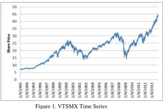
Within the study sample lie two distinct and significant bear markets following the burst of the “dot-com” bubble of late 2000 and the sub-prime mortgage bubble of late 2007 as seen in the price chart of VTSMX in Figure 1.
Figure 1. VTSMX Time Series
McEnally and Upton (1979) as well as Pettengill et al. (1995) address prior studies of the relationship between beta and realized return that have found a small or insignificant relationship between these two variables. They suggested that earlier studies failed to account for the conditional relation between beta and returns by aggregating periods of positive market return with periods of negative market return.
To address the conditional relation discussed by McEnally and Upton (1979) and Pettengill et al. (1995), the sample was divided into the following in-sample sub periods:
1. January 1, 1994 – September 7, 2000
2. September 7, 2000 - October 9, 2002
3. October 9, 2002 - October 12, 2007
4. October 12, 2007 - March6, 2009
5. March 6, 2009 – December 31, 2013
The start and end points for the test periods are the high and low points that mark the beginning and end of major market runs. For each of the above periods, the second pass of the regression was run for each measurement interval with the securities whose entire return period falls within the sub-period. The nature of beta estimation in this study does not allow for a test of the October 12, 2007 – March 6, 2009 period because it is not possible to measure a full year of post-estimation return within the sub-sample based on the method outlined above.
Following the method of Fama and French (1992), security betas were estimated in June of each year. However, in this research, the second pass of the regressions were not run on the averages of the data sorted into deciles. Instead, the second pass was run using the raw data from each securities beta estimate and post-estimation return. Because an account was made for the conditional relation between beta and return, the test periods are shorter than in previous studies. Using the raw data calculated in the first pass regression provided many more observations than would be afforded with the use of deciles. In this research, test runs of the second pass of the regression on deciles formed from the first pass produced poor statistical results, namely very large P-values and very low or negative R2. This is indicative of having too few observations and corrected by running the second pass on raw data obtained from the first pass.
Once a security beta was estimated in June, the annual return of each security was then calculated from July to the following July. For each beta estimation interval, each securities beta and post-estimation realized annual return are regressed to determine the significance of beta in predicting return. Forming portfolios in June follows Fama and French (1992) who chose this method based on the reporting of accounting data they incorporated into their model.
The central question was whether the low-beta anomaly was present for a given beta-estimation interval. The sign of the slope of the regression equations determines whether higher-beta stocks produce higher realized return for a given time-interval measurement, within a given time period. A negative sign for the regression slope demonstrates that the relationship between beta and realized return is inverse; higher beta stocks produce lower realized returns and lower beta stocks produce higher returns. A positive slope indicates a direct relationship between beta and return. For periods of positive market return, it is theorized, according to the CAPM, that the relationship is positive and the regressions will produce positive slopes. For periods of negative market return it is theorized that the relationship between beta and return is negative and will produce negative slopes. Therefore, the low beta anomaly is present only when this situation is reversed. If the low-beta anomaly is present for a given beta estimation interval, then the slope of the regression equation will be negative during periods of positive market return, or positive during periods of negative market return.
Regression analysis involves an estimation of the linear relationship between two variables. The linear regression equation is as follows in Equation 2: (Anderson et al., 2008).
y = β0 + β1X + ℇ (2)
In the linear regression equation y is the predicted value of the dependent value, β0 is the Y intercept when the line is plotted on a coordinate system, β1 is the estimated slope of the line which represents the ratio of a change in the dependent variable to a change in the independent, or predictor, variable. ℇ is the error term, or the degree to which the linear equation does not perfectly predict the value of y for a given value of X.
In order to determine the presence of the low-beta anomaly, the following hypotheses were tested for each estimation interval, in each of the test period sub-sets, as well as for the entire sample period. Therefore, the second pass of the regression was ran a total of 50 times in order to encompass each testing sub-period within an estimation interval.
The null hypothesis states that the beta coefficient is equal to zero. In a linear regression model, the beta coefficient indicates the degree to which the predictor (independent) variable influences the outcome of the dependent variable,
realized return is the dependent variable. The alternate hypothesis is a statement that the beta coefficient of the predictor variable is a non-zero number meaning that the predictor variable does explain some of the variation in y.
H0 : Equity Beta does not affect equity return. (β = 0)
Ha : Equity beta does affect equity return. (β ≠ 0)
It is necessary to test for statistical significance of estimated regression coefficients (Anderson et al., 2008). In order to do so, the regression p-value is compared to the chosen α-level.
The p-value of a regression, or any statistical test, is the probability that the statistical results obtained could also be observed if the null hypothesis were true. Therefore, a higher calculated p-value lends less support to the alternate hypothesis.
α is the level of significance associated with a hypothesis test, and is the statistical probability of rejecting a true null hypothesis. This is known as Type I error (Anderson et al., 2008). The α-level is chosen by the researcher, and is often expressed in values of .01, .05, and .10, although any value can be chosen. In financial and economic tests, .05 is commonly chosen. An α-level of .05 means that there is a 5% chance of rejecting a true null hypothesis.
With α = .05 each regression tested for a significant relationship between beta and realized return at a 95% level of confidence. When the calculated p-value is less than the chosen alpha, the null hypothesis is rejected and the alternate hypothesis is accepted. If the p-value for each regression coefficient was greater than the chosen alpha of .05 then a failure to reject the null occurred.
In this research, a rejection of the null hypothesis, H0 : β = 0, means that β is found to have a statistically significant explanatory effect on the post-estimation realized return of a security, while a failure to reject the null means that the beta coefficient has no effect on realized return.
A rejection of the null, coupled with the appropriate sign of the slope dependent on market phase, is needed in order to reach a conclusion. The theoretically supported conclusion for each second-pass regression is that the beta coefficient is significant and is positive when the market return is positive and negative when the market return is negative.
5. Results
For each of the sub-periods, the null, H0: β=0, is rejected and the alternate, H1: β≠0, accepted for estimation intervals using the previous 5 and 3 years of monthly return. All regressions showed statistically significant results using α=.05. Further, the findings are consistent with the CAPM given a conditional relationship between beta and expected return. The slope of the regression coefficient is positive for each period of positive market return and negative for each period of negative market return. For the aggregate period, the slope is positive as well.
Estimation periods using one year of monthly returns showed statistically significant and theoretically consistent results for all but one of the testing sub periods. The sub period from 2003-2006 showed a theoretically consistent, that is, positive slope due to positive market return, but statistically insignificant result at the 5% confidence level with a p-value of .0656. Therefore, for the period 2003-2006 there is a failure to reject (FTR) the null hypothesis H0:
β=0.
Using 6 months of monthly returns, FTR H0: β=0 for the testing sub period 1994-1999, as well as the aggregate period. The regression equations produced p-values of .7169 and .0561 respectively. For the remaining testing sub-periods, H0: β=0 is rejected and H1: β≠0 accepted. All testing sub-periods produced theoretically consistent slopes.
Estimating beta from five years of annual returns results in a FTR the null, H0: β=0 for 2009-2012 with a p-value of .1884. All other sub periods showed a statistically significant effect from beta with a conclusion to reject H0: β=0 and accept H1: β≠0.
The slopes of the regressions for 1999 as well as the aggregate sample period are theoretically inconsistent, and therefore evidence of the low-beta anomaly. All other sub-periods have theoretically consistent slopes.
For each of the sub-periods, the null, H0: β=0, is rejected and the alternate H1: β≠0, accepted for estimation intervals using the previous 5 years of weekly return. Regressions showed statistically significant results using α=.05. Further, the findings are consistent with the CAPM given a conditional relationship between beta and expected return. The slope of the regression coefficient is positive for each period of positive market return, and negative for each period of negative market return. For the aggregate period, the slope is positive as well. These results are consistent across the remaining methods tested for estimating beta using weekly returns: 3 years, 1 year, and 6 months.
6. Conclusion
This study did not find robust support for the low-beta anomaly, and it showed that there exist empirical differences in the estimation intervals used in constructing beta estimates. Within the twenty-year sample period from January of 1994 to December of 2013 this research covered ten different beta estimation intervals to determine whether a statistically significant and theoretically consistent relationship existed between equity beta and post-estimation realized return. In order to account for the conditional relation between beta and realized return this research independently tested four in-sample sub-periods, as well as the aggregate twenty year sample, for each estimation interval.
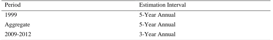
Of the fifty regressions performed, only three, the five-year, annual return regression for 1999 and the aggregate period, and the three-year, annual return for 2009-2012, supported the low-beta anomaly (summarized in Table 2), and these findings are contradicted by other beta estimation interval tests of the same periods. Four of the regressions, three-year annual return for the aggregate period, six-months of monthly return for 1994-1999 and the aggregate period, and one-year of monthly return for 2003-2006 produced statistically insignificant results and cannot be interpreted as evidence of either the CAPM or the low-beta anomaly.
Table 2. Testing Sub-Periods that Support the Low-Beta Anomaly
Period Estimation Interval
1999
Aggregate
2009-2012
5-Year Annual
5-Year Annual
3-Year Annual
While the conclusions of this study are limited in scope, it nevertheless contributes to the discussion of the quantification of the relationship between risk and return. In essence, this paper has shown that there is an empirical difference in the estimation interval used for constructing beta estimates, and that a rejection or retention of the null hypothesis does sometimes hinge on the estimation interval used; the same tests performed on different estimation intervals produce different statistical conclusions about the relationship between security beta and realized return, when using beta as the measure of a security’s risk.
Currently lacking in the literature is discussion on a supporting theory to suggest selection of one beta estimation interval over the other. Further research should be done to develop a theory of estimation interval application.
While there may be no single ideal estimation interval, it is nevertheless important to consider the implications of estimation interval choice in conducting empirical studies.
References
Abdymomunov, A., & Morley, J. (2011). Time variation of CAPM betas across market volatility regimes. Applied Financial Economics, 21, 1463-1478. https://doi.org/10.1080/09603107.2011.577010
Acker, D., & Duck, N. (2007). Reference-Day Risk and the Use of Monthly Returns Data. Journal of Accounting, Auditing, and Finance,22(4), 527-557. https://doi.org/10.1177/0148558X0702200403
Alexander, G., & Chervany, N. (1980). On the Estimation and Stability of Beta. The Journal of Financial and Quantitative Analysis,15(1), 123-137. https://doi.org/10.2307/2979022
Anderson, D., Sweeney, D., & Williams, T. (2008). Statistics for business and economics (10th ed.). Mason, OH: Thomson South-Western.
Baker, M., Bradley, B., & Taliaferro, R. (2014). The Low-Risk Anomaly: A Decomposition into Micro and Macro Effects. Financial Analysts Journal,70(2), 43-43. https://doi.org/10.2469/faj.v70.n2.2
Baker, M., Bradley, B., & Wurgler, J. (2011). Benchmarks as Limits to Arbitrage: Understanding the Low-Volatility Anomaly. Financial Analysts Journal,67(1), 40-54. https://doi.org/10.2469/faj.v67.n1.4
Black, F. (1972). Capital Market Equilibrium With Restricted Borrowing. The Journal of Business,45(3), 444-454. http://dx.doi.org/10.1086/295472
Blitz, D., Falkenstein, E., & Vliet, P. (2014). Explanations for the Volatility Effect: An Overview Based on the CAPM Assumptions. The Journal of Portfolio Management, 40(3), 61-76. https://doi.org/10.3905/jpm.2014.40.3.061
Blume, M. (1971). On the Assessment of Risk. The Journal of Finance, 26(1) 1-10. https://doi.org/10.1111/j.1540-6261.1971.tb00584.x
Bos, T., & Newbold, P. (1984). An empirical investigation of the possibility of the stochastic systematic risk of the market model. Journal of Business, 57, 35-41. http://dx.doi.org/10.1086/296222
Brailsford, T., & Josev, T. (1997). The impact of the return interval on the estimation of systematic risk.
Pacific-Basin Finance Journal,5(3), 357-376. https://doi.org/10.1016/S0927-538X(97)00006-1
Clarke, R., de Silva, H., & Thorley, S. (2006). Minimum-variance portfolios in the U.S. equity market: reducing volatility without sacrificing returns. Journal of Portfolio Management, Fall, 10-24. https://doi.org/10.3905/jpm.2006.661366
Dempsey, M. (2013). The Capital Asset Pricing Model (CAPM): The History of a Failed Revolutionary Idea in Finance? Abacus, 49, 7-23. https://doi.org/10.1111/j.1467-6281.2012.00379.x
Fabozzi, F., & Francis, J. (1978). Beta as a random coefficient. Journal of Financial and Quantitative Analysis,13, 101-116. https://doi.org/10.2307/2330525
Fama, E., & French, K. (1992). The Cross-Section of Expected Stock Returns. The Journal of Finance, 47(2), 427-465. https://doi.org/10.1111/j.1540-6261.1992.tb04398.x
Fama, E., & French, K. (1996). The CAPM is wanted, Dead or Alive. The Journal of Finance, 51(5), 1947-1958. https://doi.org/10.1111/j.1540-6261.1996.tb05233.x
Fama, E., & French, K. (2004). The Capital Asset Pricing Model: Theory And Evidence. Journal of Economic Perspectives,18(3), 25-46. https://doi.org/10.1257/0895330042162430
Fama, E., & MacBeth, J. (1973). Risk, Return, and Equilibrium: Empirical Tests. Journal of Political Economy,81, 607-636. http://dx.doi.org/10.1086/260061
Gooding, A., & O’Malley, T. (1977). Market Phase and the Stationarity of Beta. Journal of Financial and Quantitative Analysis, December (1977), 833-857. https://doi.org/10.2307/2330259
Gregory-Allen, R., Impson, M., & Karafiath, I. (1994). An Empirical Investigation of Beta Stability: Portfolios vs. Individual Securities. Journal of Business Finance & Accounting, (21)6, 909-916. https://doi.org/10.1111/j.1468-5957.1994.tb00355.x
Grind, K. (2015, May 4). The Wall Street Journal. Retrieved from
http://www.wsj.com/articles/pimcos-total-return-loses-title-as-worlds-largest-bond-fund-1430769693
Groenewold, N. & Fraser, P. (2000). Forecasting Beta: How Well Does the “Five-Year Rule of Thumb” Do? Journal of Business Finance & Accounting,27(7), 953-982. https://doi.org/10.1111/1468-5957.00341
Hagin, R., (1979). Modern Portfolio Theory. Homewood, Ill.: Dow-Jones-Irwin.
Huang, N. (2013). How to pick the best index funds. Kiplinger’s Personal Finance. Retrieved from http://www.kiplinger.com/article/investing/T041-C000-S002-how-to-pick-the-best-index-funds.html
Kothari, S., Shanken, J., & Sloan, R. (1995). Another Look at the Cross-Section of Expected Stock Returns. The Journal of Finance, 50(1), 185-224. https://doi.org/10.1111/j.1540-6261.1995.tb05171.x
Lakonishok, J., & Shapiro, A. C. (1984). Stock Returns, Beta, Variance and Size: An Empirical Analysis. Financial Analysts Journal,40(4), 36-41. https://doi.org/10.2469/faj.v40.n4.36
McEnally, R., & Upton, D. (1979) A ReExamination of the Ex Post risk-Return Tradeoff on Common Stocks. The Journal of Financial and Quantitative Analysis, 14(2) 395-419. https://doi.org/10.2307/2330511
Ohlson, J., & Rosenberg, B. (1982). Systematic risk of the CRSP equal-weighted common stock index: a history estimated by stochastic parameter regression. Journal of Business,55, 121-145. https://doi.org/10.1086/296156
Pettengill, G., Sundaram, S., & Mathur, I. (1995). The Conditional Relation between Beta and Returns. The Journal of Financial and Quantitative Analysis, 30(1), 101-116. https://doi.org/10.2307/2331255
Sharpe, W. (1964). Capital Asset Prices: A Theory of Market Equilibrium under Conditions of Risk. The Journal of Finance,19(3), 425-442. https://doi.org/10.1111/j.1540-6261.1964.tb02865.x
Sharpe, W. & Cooper, G. (1972). Risk-Return Classes of New York Stock Exchange Common Stocks, 1931-1967.
Financial Analysts Journal,28, 46-54. https://doi.org/10.2469/faj.v28.n2.46
Shefrin, H. (2001). Do investors expect higher returns from safer stocks than from riskier stocks? Journal of Psychology and Financial Markets, 2(4), 176-181. http://dx.doi.org/10.1207/S15327760JPFM0204_1
Theobald, M. (1981). Beta Stationarity and Estimation Period: Some Analytical Results. Journal of Financial and Quantitative Analysis, 16(5), 747-757. https://doi.org/10.2307/2331058
Vanguard.com. (n.d.). Retrieved from
https://personal.vanguard.com/us/funds/snapshot?FundId=0085&FundIntExt=INT
Vanguard.com. (n.d.). Retrieved from