Methods for Volumetric Reconstruction of Visual Scenes
GREGORY G. SLABAUGH
Intelligent Vision and Reasoning Department, Siemens Corporate Research, Princeton, NJ 08540
W. BRUCE CULBERTSON, THOMAS MALZBENDER
Visual Computing Department, Hewlett-Packard Laboratories, Palo Alto, CA 94304
{
bruce culbertson, tom malzbender
}
@hp.com
MARK R. STEVENS
Charles River Analytics Inc., Cambridge, MA 02138
RONALD W. SCHAFER
Center for Signal and Image Processing, Georgia Institute of Technology, Atlanta, GA 30318
Abstract
In this paper, we present methods for 3D volumetric reconstruction of visual scenes photographed by multiple calibrated cameras placed at arbitrary viewpoints. Our goal is to generate a 3D model that can be rendered to syn-thesize new photo-realistic views of the scene. We improve upon existing voxel coloring / space carving approaches by introducing new ways to compute visibility and photo-consistency, as well as model infinitely large scenes. In particular, we describe a visibility approach that uses all possible color information from the photographs during reconstruction, photo-consistency measures that are more robust and/or require less manual intervention, and a volu-metric warping method for application of these reconstruc-tion methods to large-scale scenes.
Keywords
Scene reconstruction, voxel coloring, space carv-ing, photo-consistency, histogram intersection, volumetric warping
1
Introduction
In this paper, we consider the problem of reconstructing a 3D model of a scene of unknown geometric structure us-ing a set of photographs (also called reference views) of the scene taken from calibrated and arbitrarily placed cameras. Our goal is to reconstruct geometrically complex scenes
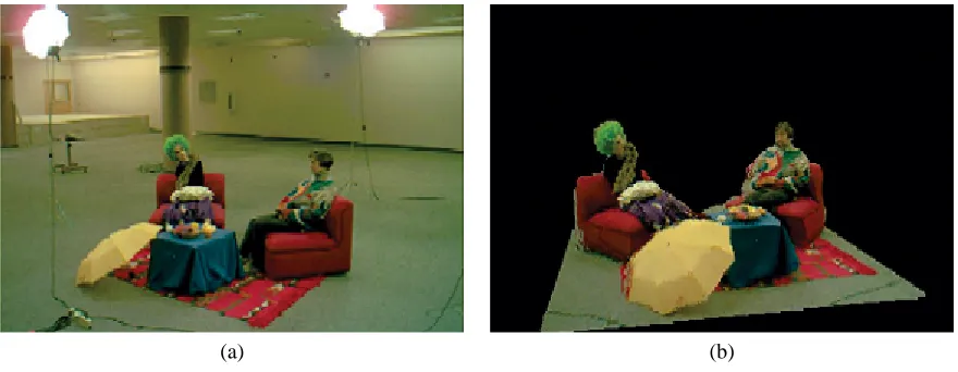
using a set of easily obtained photographs taken with inex-pensive digital cameras. We then project this reconstructed 3D model to virtual viewpoints in order to synthesize new views of the scene, as shown in Figure 1.
To accomplish this task, we have developed methods that improve upon the quality, usability, and applicabil-ity of existing volumetric scene reconstruction approaches. We present innovations in the computation of visibility and photo-consistency, which are two crucial aspects of this class of algorithms. One of our visibility approaches mini-mizes photo-consistency evaluations, which results in effi-cient computation, and our histogram intersection method of computing photo-consistency requires almost no user in-tervention. We also present a volumetric warping approach designed to reconstruct infinitely large scenes using a finite number of voxels. These techniques are aimed at bringing volumetric scene reconstruction out of the laboratory and towards the reconstruction of complex, real-world scenes.
1.1
Related Work
re-Figure 1: One of 24 reference views of our “Ceevah” data set (a) and a new view synthesized after scene reconstruction (b).
quire user interaction [11, 41]. In this paper, we are inter-ested in a more general case, for which a scene of unknown geometric structure is photographed from any number of arbitrarily placed cameras. We are most interested in tech-niques that require minimal interaction with the user.
In the literature, several methods to represent a visual scene have been proposed, including layered depth im-ages [40], surface meshes, surfels [6, 34], light fields [18, 26], etc. In this paper, we focus on volumetric representa-tions, which provide a topologically flexible way to char-acterize a 3D surface inferred from multiple images. If desired, a voxel-based surface can be converted into any of the above representations with relative ease.
Due to the large number of scene reconstruction ap-proaches, it would be impossible to provide a comprehen-sive review here; see [12, 43] for a survey of volumetric approaches. Techniques such as multi-view stereo [17, 32] and structure from motion [1, 20, 35] have been quite suc-cessful at reconstructing 3D scenes. These methods com-pute and then triangulate correspondences between views to yield a set of 3D points that are then fit to a surface. The effectiveness of these reconstruction methodologies relies upon accurate image-space correspondence match-ing. Such matching typically falters as the baseline be-tween views increases since the effects of occlusion and perspective are difficult to model in image space when the scene geometry is unknown. Consequently, many of these methods are not well suited to the arbitrary placement of cameras.
A level set approach to the scene reconstruction prob-lem has been proposed by Faugeras and Keriven [16]. A surface initially larger than the scene is evolved using par-tial differenpar-tial equations to a successively better approx-imation of true scene geometry. Like the approaches we
present in this paper, this level set method can employ ar-bitrary numbers of images, account for occlusion correctly, and deduce arbitrary topologies.
Perhaps the simplest class of volumetric multi-view reconstruction methods are visual hull approaches [25, 29, 47]. The visual hull, computed from silhouette im-ages, is an outer-bound approximation to the scene ge-ometry. Algorithms that compute the visual hull are ap-plicable to scenes with arbitrary BRDFs as long as fore-ground/background segmentation at each reference view is possible, and are relatively simple to implement since vis-ibility need not be modeled when reconstructing the scene geometry.
While a visual hull can be rendered to produce new views of the scene, typically the visual hull geometry is not very accurate. This can diminish the photo-realism when new views are synthesized. To increase the geometric ac-curacy, more information than silhouettes must be used during reconstruction. Color is an obvious source of such additional information. Many researchers have attempted to reconstruct 3D scenes by analyzing colors across multi-ple viewpoints. Specifically, they have sought a 3D model that, when projected to the reference views, reproduces the photographs.
Reconstructing such a model requires a photo-consistency check, which determines if a point in 3D space is consistent with the photographs taken of the scene. In particular, a point is photo-consistent [39, 24] if:
• It does not project to background, if the background is known.
photograph.
Kutulakos and Seitz [24] state that surfaces that are not transparent or mirror-like reflect light in a coherent man-ner; that the color of light reflected from a single point along different directions is not arbitrary. The photo-consistency check takes advantage of this fact to eliminate visible parts of space that do not contain scene surfaces.
This reconstruction problem is ill-posed in that, given a set of photographs and a photo-consistency check, there are typically multiple 3D models that consist of photo-consistent points. In their insightful work, Kutulakos and Seitz [24] introduce the photo hull, which is the largest shape that contains all reconstructions in the equivalence class of photo-consistent 3D models. For a given mono-tonic photo-consistency check1, the photo hull is unique,
and is itself a reconstruction of the scene. Since we model points with voxels, the photo hull is found by identify-ing the spatially largest volume of voxels that are photo-consistent with all reference views.
When computing the photo hull, we have found that the quality of the result depends heavily on two factors. They are:
1. Visibility: The method of determining of the pixels from which a voxel V is visible. We denote these pixelsπV.
2. Photo-consistency test: A function that decides, based onπV, whether a surface exists atV.
In the algorithm presented in the next paragraph, we will see that visibility and photo-consistency are inter-related and, as a result, multiple passes must in general be made over the voxels to find the photo hull.
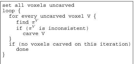
Volumetric methods for finding the photo hull adopt the following approach. First, a voxel space is defined that contains, by a comfortable margin, the portion of the scene to be reconstructed. During reconstruction, the voxels are either completely transparent or opaque; initially, they are all opaque. Voxels that are visible to the cameras are checked for photo-consistency, and the inconsistent voxels are carved, i.e., their opacity is set to transparent. Carving one voxel typically changes the visibility of other opaque voxels. Since the photo-consistency of a voxel is a func-tion of its visibility, the consistency of an uncarved voxel must be rechecked whenever its visibility changes. The algorithm continues until all visible, uncarved voxels are photo-consistent. This set of voxels, when rendered to the reference views, reproduces the photographs and is there-fore a model that resembles the scene. Pseudocode is pro-vided in Figure 2.
1We will discuss monotonicity in Section 2.
set all voxels uncarved loop {
for every uncarved voxel V {
find πV
if (πV is inconsistent)
carve V
}
if (no voxels carved on this iteration) done
}
Figure 2: Generic pseudocode for reconstructing the photo hull.
The Voxel Coloring algorithm of Seitz and Dyer [39] re-constructs the photo hull for scenes photographed by cam-eras that satisfy the ordinal visibility constraint, which re-stricts the camera placements so that the voxels can be vis-ited in an order that is simultaneously near-to-far relative to every camera. Typically, this condition is met by placing all the cameras on one side of the voxel space, and process-ing voxels usprocess-ing plane that sweeps through the volume in a direction away from the cameras. Under this constraint, visibility is simple to model using occlusion bitmaps [39]. Voxel Coloring is elegant and efficient, but the ordi-nal visibility constraint is a significant limitation, since it means that cameras cannot surround the scene. Kutu-lakos and Seitz [23] present what we call the Partial Vis-ibility Space Carving (PVSC) algorithm, which repeat-edly sweeps a plane through the volume in all six axis-aligned directions. For each plane sweep, only the subset of cameras that are behind the plane are used in the photo-consistency check. This approach permits arbitrary cam-era placement, which is a significant advantage over Voxel Coloring. However, when evaluating a voxel’s photo-consistency, it uses pixels from only a subset of the total cameras that have visibility of the voxel. To address this issue, Kutulakos and Seitz [24] subsequently include some additional per-voxel bookkeeping that accumulates the vis-ible pixels in the voxel’s projection as the plane is swept in all six axis-aligned directions. On the sixth sweep, the full visibility of the voxel is known and considered in the photo-consistency check. We call this version of their al-gorithm Full Visibility Space Carving (FVSC).
and non-Lambertian surfaces [6, 7]. Vedula et al. [50] and Carceroni and Kutulakos [6] propose carving algo-rithms for reconstructing time-varying scenes. Slabaugh et al. [44] present an epipolar approach to constructing view-dependent photo hulls at interactive rates.
1.2
Contributions
This paper presents contributions in three areas; visibil-ity, photo-consistency, and the modeling of infinitely large scenes. We discuss each below.
As stated above, visibility is a vital part of any algorithm that reconstructs the photo hull. In Section 2 we present a scene reconstruction approach, Generalized Voxel Color-ing (GVC), which introduces novel methods for computColor-ing visibility during reconstruction. These methods support ar-bitrary camera placement and place minimal requirements on the order in which voxels are processed, unlike plane sweep methods [39, 24]. We show that one of our new methods minimizes photo-consistency checks. We also demonstrate how full visibility can result in more accurate reconstructions for real-world scenes.
The photo-consistency test is the other crucial part of an algorithm that reconstructs the photo hull. In Section 3 we introduce two novel photo-consistency tests for Lam-bertian scenes. The first is an adaptive technique that ad-justs the photo-consistency test so that surface edges and textured surfaces can be more accurately reconstructed. The second is based on color histograms and treats multi-modal color distributions in a more principled way that ear-lier approaches. In addition, our histogram-based photo-consistency test requires little parameter tuning.
Reconstruction of large-scale scenes that contain ob-jects both near to and far from the cameras is a challenging problem. Modeling such a scene with a fixed resolution voxel space is often inadequate. Using a high enough res-olution for the foreground may result in an unwieldy num-ber of voxels that becomes prohibitive to process. Using a lower resolution, more suitable to the background, may result in an insufficient resolution for the foreground. In Section 4 we present a volumetric warping approach that represents infinitely large scenes with a finite number of voxels. This method simultaneously models foreground objects, background objects, and everything in between, using a voxel space with variable resolution. Using such a voxel space in conjunction with our GVC approach, we reconstruct and synthesize new views of a large outdoor scene.
We note that some of the content of this paper has ap-peared in previous workshop and conference papers [9, 42, 46].
rithms2that we collectively call Generalized Voxel Carv-ing (GVC). They differ from each other, and from earlier space carving algorithms, primarily in the means they com-pute visibility. The earlier methods require the voxels to be scanned in plane sweeps, whereas GVC scans voxels in a more general order. GVC represents just visible surface voxels in its main data structure, reducing both computa-tion and storage. GVC accounts for visibility in a way that very naturally accommodates arbitrary camera placement and allows full voxel visibility to be computed efficiently. The first GVC algorithm, GVC-IB, uses less memory than the other. It also uses incomplete visibility information during much of the reconstruction yet, in the end, com-putes the photo hull using full visibility. The other GVC algorithm, GVC-LDI, uses full visibility at all times, which greatly reduces the number of photo-consistency checks re-quired to produce the photo hull. We show that the use of full visibility results in better reconstructions than those produced by earlier algorithms that only use partial visibil-ity.
As mentioned earlier, carving one voxel can change the visibility of other voxels, so visibility must be calculated frequently while reconstructing a photo hull. Because of self-occlusion in the scene, visibility is complex and po-tentially costly to compute. Thus, an efficient means of computing visibility is a key element of any practical space carving algorithm, including our GVC algorithms.
As a space carving algorithm begins a reconstruction, it carves voxels based on the visibility of a model that looks nothing like the final photo hull. One might therefore won-der: could the algorithm carve a voxel that belongs in the photo hull? To answer this question, consider the follow-ing two insights, based on Seitz and Dyer [39]. First, since voxels change from opaque to transparent during recon-struction, and never the reverse, the visibility of the remain-ing voxels can only increase. In particular, ifSis the set of pixels that have an unoccluded view of an uncarved voxel at one point in time and ifS0 is the set of such pixels at a later point in time, thenS ⊆ S0. Second, Seitz and Dyer make an unstated assumption that the consistency test is
monotonic, meaning for any two sets of pixelsS andS0 withS ⊆ S0, if S is inconsistent, thenS0 is also incon-sistent. These two facts imply that carving is conservative: no voxel will ever be carved if it would be photo-consistent in the final model. (Although carving with non-monotonic consistency tests is not in general conservative, we show in
2Throughout this paper, we will use the term “space carving
Section 3 that such tests can nevertheless yield good look-ing reconstructions.)
Both GVC-IB and GVC-LDI maintain a surface voxel list (SVL), a list of the surface voxels in the current model that are visible from the cameras. For box-shaped voxel spaces that contain none of the cameras, we typically ini-tialize the SVL with the outside layer of voxels. We have used ad hoc methods to initialize the SVL when we used more complicated voxel spaces, as in Section 4. When a voxel is carved, we remove it from the SVL. We also add to the SVL any voxels that are adjacent to the carved voxel and that have not been previously carved; this pre-vents holes from being introduced into the surface repre-sented by the SVL. As described below, we give each voxel a unique ID number. We use a hash table to find the voxel with a given ID in the SVL. The SVL can also be scanned sequentially.
2.1
The GVC-IB Algorithm
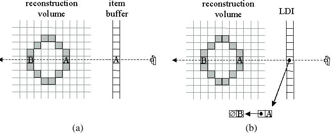
The GVC-IB algorithm maintains visibility using an item buffer [51] for each reference image. An item buffer is defined as follows: for each pixelP in a reference im-age, an item buffer, shown in Figure 3a, stores the voxel ID of the closest voxel that projects toP(if any). An item buffer is computed by rendering the voxels into the ref-erence image usingz-buffering, but storing voxel IDs in-stead of colors. As with earlier space carving algorithms, it is assumed that at most one voxel is visible from any pixel. Therefore, we make no attempt to model blended colors that arise from transparency [10] or depth disconti-nuities [48].
Pseudocode for GVC-IB appears in Figure 4. Once valid item buffers have been computed for the images, their pixels are then scanned. During the scan, if a valid voxel ID is found in a pixel’s item buffer value, then the pixel’s color is accumulated into the voxel’s color statistics.
When the pixel scanning is complete, the SVL is scanned and each voxel is tested for consistency, based on the collected color statistics. If a voxel is found to be in-consistent, it is carved and removed from the SVL. After a voxel is carved, the visibility of the remaining SVL voxels potentially changes, so all the color statistics must be con-sidered out-of-date. At this point, it might seem natural to recompute the item buffers and start the process all over. However, because the item buffers are time-consuming to compute, we delay updating them. Although the visibility found using out-of-date item buffers is no longer valid for the current model, it is still valid for a superset of the cur-rent model. Because carving is conservative, no consistent voxels will be carved using the out-of-date color statistics, though some voxels that should be carved might not be. When the entire SVL has been scanned and all voxels with inconsistent color statistics have been carved, then we
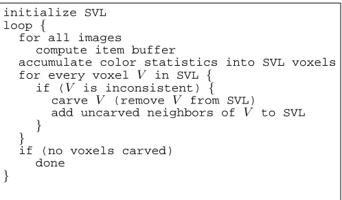
re-initialize SVL loop {
for all images
compute item buffer
accumulate color statistics into SVL voxels for every voxel V in SVL {
if (V is inconsistent) {
carve V (remove V from SVL)
add uncarved neighbors of V to SVL
} }
if (no voxels carved) done
}
Figure 4: GVC-IB pseudocode.
compute the item buffers and begin again. These iterations continue until, during some iteration, no carving occurs. At this point, the SVL is entirely consistent, based on up-to-date visibility, so the SVL is in fact the photo hull.
Profiling GVC-IB revealed that nearly all the runtime is spent rendering item buffers. This suggested two ways to accelerate the algorithm. Since each item buffer is in-dependent of the others, they can be rendered in parallel on a multi-CPU computer. Using two CPUs and several image sets, we measured runtime reductions between 46% and 48% compared to a uniprocessor. Next, we tried ren-dering the item buffers with a hardware graphics accel-erator. This resulted in runtime reductions between 56% and 63%. GVC-IB (and GVC-LDI) can also be executed in a coarse-to-fine manner, as described in [36]. We have seen runtime reductions of approximately 50% using such multi-resolution voxel spaces. These efficiencies can be combined for faster reconstructions.
2.2
The GVC-LDI Algorithm
Figure 3: The data structures used to compute visibility. An item buffer (a) is used by GVC-IB and records the ID of the surface voxel visible from each pixel in an image. A layered depth image (LDI) (b) is used by GVC-LDI and records all surface voxels that project onto each pixel.
instead of item buffers, GVC-LDI can efficiently and im-mediately update the visibility information when a voxel is carved and also can precisely determine the voxels whose visibility has changed.
Unlike the item buffers used by the GVC-IB method, which record at each pixel P just the closest voxel that projects ontoP, the LDIs store at each pixel a list of all the surface voxels that project ontoP. See Figure 3b. These lists are sorted according to the distance from the voxel to the image’s camera. The head of an LDI list stores the voxel closest toP, which is the same voxel an item buffer would store. The LDIs are initialized by rendering the SVL voxels into them.
Using the LDIs, the set of pixelsπV from which a voxel V is visible can be found as follows. V is scan converted into each reference image to find its projection (without regard to visibility). For each pixelP inV’s projection, if the voxel ID at the head ofP’s LDI equalsV’s ID, then P is added toπV. OnceπV is computed,V’s consistency
can be determined by testingπV.
The uncarved voxels whose visibility changes when an-other voxel is carved come from two sources:
• They are inner voxels adjacent to the carved voxel and become surface voxels when the carved voxel be-comes transparent. See Figure 5a.
• They are already surface voxels (hence they are in the SVL and LDIs) and are often distant from the carved voxel. See Figure 5b.
Voxels in the first category are trivial to identify since they are next to the carved voxel. Voxels in the second cat-egory are impossible to identify efficiently in the GVC-IB method; hence, that method must repeatedly evaluate the entire SVL for color consistency. In GVC-LDI, vox-els in the second category can be found easily with the
aid of the LDIs; they will be the second voxel on the LDI list for some pixel in the projection of the carved voxel. GVC-LDI keeps a list of the SVL voxels whose visibility has changed, called the changed visibility SVL (CVSVL). These are the only voxels whose consistency must be checked. Carving is finished, and the photo hull is found, when the CVSVL is empty.
When a voxel is carved, the LDIs (and hence the vis-ibility information) can be updated immediately and effi-ciently. The carved voxel can be easily deleted from the LDI list for every pixel in the voxel’s projection. The same process automatically updates the visibility information for the second category of uncarved voxels whose visibility has changed; these voxels move to the head of LDI lists from which the carved voxel has been removed and they are also added to the CVSVL. Inner voxels adjacent to the carved voxel are pushed onto the LDI lists for pixels they project onto. As a byproduct of this process, the algorithm learns if the voxel is visible; if it is, it is put on the CVSVL. Pseudocode for GVC-LDI is given in Figure 6.
2.3
GVC Reconstruction Results
We now present experimental results to demonstrate our GVC algorithms, and provide, for side-by-side compari-son, results obtained with Space Carving. As discussed in Section 1.1, there are two versions of the Space Carving al-gorithm: Partial Visibility Space Carving (PVSC) and Full Visibility Space Carving (FVSC). As will be shown, PVSC produces less accurate results than GVC and FVSC. There-fore, we will focus more on comparing GVC to FVSC.
2.3.1 Comparison with Partial Visibility Space Carv-ing
(a) (b)
Figure 5: When a voxel is carved, there are two categories of other voxels whose visibility changes: (a) inner voxels that are adjacent to the carved voxel and (b) voxels that are already on the SVL and are often distant from the carved voxel.
initialize SVL for all images compute LDI
place all voxels in SVL onto CVSVL while (CVSVL not empty) {
choose a voxel V from CVSVL remove V from CVSVL
scan convert V to find πV if (πV is not consistent) {
carve V (remove from SVL, LDIs) for all inner neighbors U of V
add U to SVL, CVSVL, LDIs
for voxels U that move to head of LDIs add U to CVSVL
} }
Figure 6: GVC-LDI pseudocode.
had accuracy of a maximum 1.2 pixels of reprojection er-ror for the points used in the calibration. We reconstructed the scene using a 75 x 71 x 33 voxel volume. New views synthesized from the GVC-IB and PVSC reconstructions are shown in Figure 8.
The PVSC image is considerably noisier and more dis-torted than the GVC image, a trend we observed with all data sets we tested. In general, PVSC produces less ac-curate reconstructions than GVC, since, when computing photo-consistency, PVSC does not use the full visibility of the scene, unlike GVC. During a plane sweep, the cameras that are ahead of the plane are not considered by the PVSC algorithm even though those cameras might have visibility of voxels on the plane. Since photo-consistency is
deter-mined using a subset of the available color information, the photo-consistency test sometimes fails to produce the proper result had the full visibility been considered. For some data sets, we found the PVSC runs faster, while for others, GVC runs faster. However, PVSC always requires less memory than GVC-IB or GVC-LDI.
Additional comparisons between GVC and PVSC ap-pear in [9].
2.3.2 Comparison with Full Visibility Space Carving
Next, we present results of running GVC-IB, GVC-LDI, and Full Visibility Space Carving (FVSC) on two data sets we call “toycar” and “ghirardelli”. In particular, we present runtime statistics and provide images synthesized with FVSC and our algorithms. The experiments were run on a computer with a 1.5 GHz Pentium 4 processor and 768 MB of RAM.
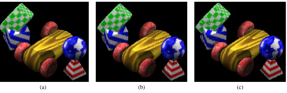
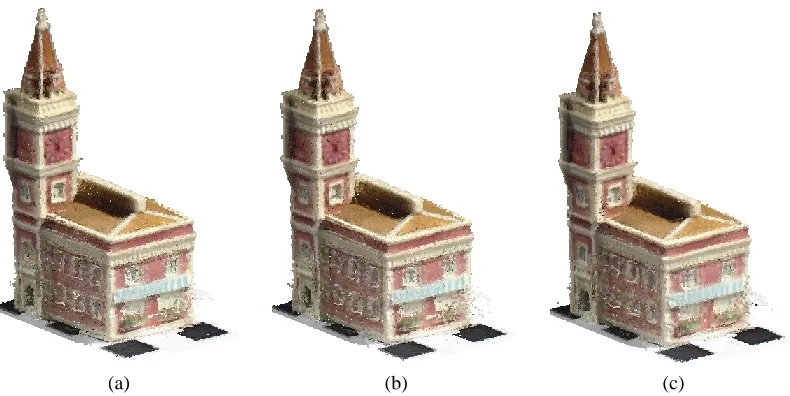
The toycar and ghirardelli data sets are quite different in terms of how difficult they are to reconstruct. The toy-car scene is ideal for reconstruction. The seventeen 800 x 600 pixel images are computer-rendered and perfectly cal-ibrated. The colors and textures make the various surfaces in the scene easy to distinguish from each other. Two of our toycar reference views are shown in Figure 9. In con-trast, the seventeen 1152 x 872 ghirardelli images are im-perfectly calibrated photographs of an object that has sig-nificant areas with relatively little texture and color varia-tion. Two of our ghirardelli reference views are shown in Figure 11.
Figure 7: Two of the fifteen input images of the bench scene.
(a) (b)
Figure 8: New views projected from reconstructions of the bench scene. The image on the left was created with GVC-IB. The image on the right was created with Partial Visibility Space Carving. The PVSC image is considerably noisier and more distorted than the GVC-IB image.
voxel volume. The reconstruction of the ghirardelli data set occurred in a 168 x 104 x 256 voxel volume; note this resolution is significantly higher than that used to recon-struct the toycar scene. New views synthesized from re-constructions obtained using the GVC-IB, GVC-LDI, and FVSC algorithms are shown in Figures 10 and 12 for the toycar and ghirardelli data sets, respectively. The three re-constructions in each figure are not identical because we used a photo-consistency test (the adaptive standard devia-tion test that will be discussed in Secdevia-tion 3.2.1) that is not monotonic. Therefore, the order in which the voxels were processed affected the final result. However, for each data set, the three reconstructions are comparable in terms of quality.
There were significant differences between the algo-rithms in terms of runtime statistics, as shown in Table 1. The “Checks” column in the table indicates the number of
(a) (b)
Figure 9: Two of the seventeen images of the toycar scene.
(a) (b) (c)
Figure 10: New views of the toycar scene generated by rendering the GVC-IB (a), GVC-LDI (b), and FVSC (c) reconstruc-tions.
Data Set Algorithm Checks Time (m:s) Memory
Toycar FVSC 25.8 M 32:31 156 MB
Toycar GVC-IB 3.1 M 36:16 74 MB
Toycar GVC-LDI 2.2 M 29:16 399 MB
Ghir. FVSC 154 M 2:35:43 337 MB
Ghir. GVC-IB 12.1 M 2:01:27 154 MB Ghir. GVC-LDI 4.5 M 0:47:10 275 MB
Table 1: Runtime statistics for the toycar and ghirardelli data sets.
more visibility. In particular, GVC-LDI always uses full visibility each time a voxel’s photo-consistency is checked.
The “Time” column in Table 1 indicates the amount of time required to complete the reconstruction. For the
toycar data set, the GVC algorithms were slightly faster than FVSC. Although GVC processes fewer voxels, the additional overhead required to maintain the visibility data structures does not result in a significantly faster runtime. However, for the Ghirardelli data set, the efficiency of GVC-LDI’s relatively complex data structures more than compensates for the time needed to maintain them. Be-cause GVC-LDI finds all the pixels from which a voxel is visible, it can carve many voxels sooner, when the model is less refined, than GVC-IB. Furthermore, after carving a voxel, GVC-LDI only reevaluates the few other voxels whose visibility has changed. Consequently, GVC-LDI is faster than GVC-IB by a large margin. For FVSC, the large number of photo-consistency checks results in a slower runtime.
Figure 11: Two of the seventeen reference views of the ghirardelli scene.
(a) (b) (c)
Figure 12: New views of the ghirardelli scene generated by rendering the GVC-IB (a), GVC-LDI (b), and FVSC (c) reconstructions.
input images in memory. As described in [24], for Lam-bertian scenes, FVSC additionally stores color statistics for each voxel in the voxel space. This grows asO(N3),
whereN is the number of voxels along one dimension of the voxel space. Additionally, we store the one of six parti-tions [24] of space that each camera lies in for each voxel. This storage is also O(N3). We note that the partitions
could be computed on the fly (i.e., requiring no storage) at the expense of runtime. However, in our experiments, we opted for a faster runtime. Unlike FVSC, the voxel res-olution has little bearing on the memory requirements for GVC-IB and GVC-LDI. GVC-IB requires equal amount
of memory for the images and the item buffers. The LDIs dominate the memory usage in GVC-LDI and consume an amount of memory roughly proportional to the number of image pixels times the depth complexity of the scene. The SVL and CVSVL data structures used by GVC-IB and GVC-LDI requireO(N2)storage, and are relatively
2.4
Summary
In this section we presented our Generalized Voxel Coloring algorithms, GVC-IB and GVC-LDI. These ap-proaches support arbitrary camera placement and recon-struct the scene using full visibility. We demonstrated that methods like GVC that use full visibility result in more accurate reconstructions than those that use partial visibil-ity. The GVC-IB algorithm is memory efficient, while our GVC-LDI algorithm reconstructs the scene using a mini-mal number of photo-consistency checks, which, for many scenes, results in a faster reconstruction.
3
Photo-Consistency Tests
When reconstructing a scene using a space carving al-gorithm, there are two key factors that affect the quality of the reconstructed model. The first is the visibility that is computed for the voxels. In the previous section we demonstrated that using full visibility produces better qual-ity reconstructions than using only partial visibilqual-ity. The second factor is the test that is used to judge the photo-consistency of voxels.
The section begins by describing the likelihood ratio test, the first consistency test that was proposed for space carving. We then describe several of the most straight-forward, and perhaps obvious, candidate tests. Next, we present two tests that we have developed, the adaptive stan-dard deviation test and the histogram test. These two tests have consistently yielded the best results in our new view synthesis application, and one of the tests has the added advantage of requiring little or no parameter adjustment. Finally, we present results that show some color spaces are better than others for space carving.
We have provided Figure 13 for comparison of the con-sistency tests and color spaces. It shows reconstructions performed with identical programs, aside from the tests or color spaces being compared. All the reconstructions in the figure use the same “shoes” data set, consisting of 30
1536×1024images, but the results are consistent with other data sets we have tried. The reconstructions have been rendered to an identical viewpoint that is different from any of the input images used in the reconstructions. Parameters used in the tests were tuned to minimize holes in the calibration target that serves as the floor of the scene. O¨guz ¨Oz¨un [33] has also compared consistency tests and had similar success with the two tests we developed.
Kutulakos and Seitz [24] have stated that the photo hull, the set of all photo consistent voxels, provides “the tightest possible bound on the shape of the true scene that can be inferred from N photographs”. However, different photo consistency tests lead to different photo hulls, many of which do not resemble the scene. If there is a voxel that belongs in a reconstruction but is judged by the test to be inconsistent, then space carving carves the voxel from the
model. Worse, because the voxel is then considered trans-parent, the algorithm can draw incorrect conclusions about which images see the remaining uncarved voxels, leading to more incorrect carving. Figure 15b shows an example of this problem. The consistency test just described can be thought of as being too strict for declaring voxels that be-long in the model to be inconsistent. Tests can also be too lenient, declaring voxels to be consistent when they do not belong in the model; this can lead to voxels that appear to float over a reconstructed scene. A single consistency test can simultaneously be both too strict and too lenient, cre-ating holes in one part of a scene and flocre-ating voxels else-where. The reconstructions in Figure 13 all demonstrate this to varying degrees.
In most space carving implementations there has been an implicit assumption that the pixel resolution is greater than the voxel resolution—that is, a voxel projects to a number of pixels in at least some of the images. We lieve this is reasonable and expect the trend to continue be-cause: 1) runtime grows faster with increasing voxel res-olution than it does with increasing pixel resres-olution, and 2) the resolution of economical and readily available cam-eras keeps growing. We make use of this assumption in the adaptive standard deviation and histogram consistency tests. Steinbach et al. [45] have reported that they obtained better reconstructions when they precisely computed the projections of voxels into images, rather than using approx-imations, like splats. We have observed the same effect and therefore use scan conversion to determine voxel pro-jections. We make the assumption in this section that the scenes being reconstructed are approximately Lambertian, and we use the RGB color space, except where noted.
3.1
Monotonic Consistency Tests
Kutulakos and Seitz assume monotonic consistency tests will be used with space carving. When such tests and full visibility are employed, space carving is guaranteed to yield the photo hull, the unique photo-consistent model that is a superset of all other photo-consistent models.
Seitz and Dyer [39] determine the consistency of a voxel V using the likelihood ratio test (LRT):
(n−1)s2πV < τ (1)
whereπV is the set of pixels from whichV is visible,s πV
is the standard deviation of the colors of the pixels inπV,
nis the cardinality ofπV, andτis a threshold that is
(d) (e) (f) (g)
Figure 13: Reconstructions of the shoes data set using different consistency tests. (a) is a photograph of the scene that was not used during reconstruction. (b) was reconstructed using the likelihood ratio test, (c) using the bounding box test, (d) using standard deviation, (e) using standard deviation and the CIELab color space, (f) using the adaptive standard deviation test, and (g) using the histogram test.
The next two consistency tests we describe are mono-tonic and lack LRT’s sensitivity to the number of pixels that view voxels. Perhaps the most obvious choice for a monotonic consistency test is:
max{dist(color(p1), color(p2))|p1, p2∈πV}< τ (2)
wheredistis theL1orL2norm in color space. The
disad-vantages of this test are its computational complexity and its sensitivity to pixel noise. The bounding box test is a simple, related test with low computational complexity. In this test, a voxelV is checked for consistency by compar-ing a threshold to the length of the great diagonal of the axis-aligned bounding box, in RGB space, of the colors of the pixels in πV. Disadvantages of the bounding box test
are that it is a somewhat crude measure of color consis-tency and it is sensitive to pixel noise. A reconstruction performed with this test, shown in Figure 13c, produced more floating voxels than LRT but also recovered some de-tail that LRT missed.
3.2
Non-monotonic Consistency Tests
We can easily think of plausible consistency tests, for example tests that threshold common statistics like stan-dard deviation:
sπV < τ (3)
Unfortunately, many such tests are not monotonic, includ-ing thresholded standard deviation. When space carvinclud-ing is used with non-monotonic consistency tests, it can carve a voxel that might be consistent in the final model. The algorithm can also converge to different models depend-ing upon the order in which the voxels are processed, so there is no unique photo hull corresponding to such tests. However, this is not necessarily a disadvantage if the objec-tive is to produce models that closely resemble the scene. In fact, among the tests we have tried, the two that have consistently produced the best looking models, the adap-tive standard deviation test and the histogram test, are not monotonic. The reconstruction shown in Figure 13d, produced using thresholded standard deviation, demon-strates that non-monotonic tests can yield reasonable mod-els. The test produced fewer floating voxels than LRT and the bounding box test, and recovered some detail that LRT missed.
3.2.1 An Adaptive Consistency Test
(a) (b)
(c) (d)
Figure 14: Handling texture and edges. In (a), a voxel represents a homogeneous region, for which bothsπV and
s are small. In (b) and (c), a voxel represents a textured region and an edge, respectively, for which bothsπV ands
are large. In (d), a voxel representing free space has a large sπV and smalls.
needed to reconstruct such surfaces. The same scenes can also include surfaces with little or no color variation. Such regions require a low threshold to minimize cusping and floating voxels. Fortunately, we can measure the amount of color variation on a surface by measuring the amount color variation the surface projects to in single images.
This suggests that it would be beneficial to use an adap-tive threshold that is proportional to the color variation seen from single images. This is illustrated in Figure 14. LetπVi be the set of pixels in imageifrom which voxelV is vis-ible, letsπV
i be the standard deviation ofπ
V
i and letsbe
the average ofsπV
i for all imagesifrom whichV is visible.
In (a), (b) and (c) in the figure, where the voxel is on the surface, note thatsπV andsare both simultaneously either
small or large. In (d), where the voxel is not on the surface, sis small andsπV is large.
We constructed an adaptive consistency test, which we call the adaptive standard deviation test (ASDT), as fol-lows:
sπV < τ1+τ2s (4)
where τ1 and τ2 are thresholds whose values are
deter-mined experimentally. ASDT is the same as the thresh-olded standard deviation test of Equation 3 except for the τ2sterm.
Figure 15 shows a data set for which thresholded stan-dard deviation, regardless of threshold, failed to recon-struct the scene, yet ASDT produced a reasonable model.
(a) (b) (c)
Figure 15: Figure (a) is a reference image from our El data set, (b) shows the best reconstruction obtained using thresholded standard deviation, and (c) shows a reconstruc-tion obtained using the adaptive standard deviareconstruc-tion test.
Figure 13f shows an ASDT reconstruction that is superior to reconstructions produced by any of the other consistency tests we have described so far. Note that the ASDT model has fewer floating voxels as well as fewer holes than the other models. A disadvantage of ASDT is the experimen-tation that is required to find the values ofτ1 andτ2that
produce the best reconstruction.
3.2.2 A Histogram-Based Test
Since a voxel often represents a part of a surface that crosses color boundaries or includes significant texture, it can be visible from pixels whose colors have a complex, multi-modal distribution. A few parameters of a distribu-tion, such as the variance and standard deviation used by the previous tests, can only account for second order statis-tics of the distribution. Furthermore, such parameters make assumptions about the distributions, for example standard deviation accurately characterizes only Gaussian distribu-tions. The multi-modal color distributions that we would like to characterize are unlikely to conform to any such as-sumptions. In contrast, histograms are nonparametric rep-resentations that can accurately describe any distribution. This inspired us to develop a consistency test that uses his-tograms. The test produces excellent reconstructions and has the additional advantage of requiring little or no pa-rameter adjustment.
∀i,jHist(πVi )
\
Hist(πVj)6=∅ i6=j (5) Therefore, a single pair of views can cause a voxel to be declared inconsistent if the colors they see at the voxel do not overlap. We use a 3D histogram over the complete color space. Furthermore, we have found that eight bins per channel are adequate for acceptable reconstructions; this yields 512 bins (8×8×8) for each image of each voxel.
We made several optimizations to minimize the runtime and memory requirements related to our consistency test. Notice that the histogram intersection only needs to test which histogram bins are occupied. Hence, only one bit is required per bin, or512 bits per histogram. Histogram intersection can be tested with AND operations on com-puter words. Using 32-bit words, only16AND instruc-tions are needed to intersect two histograms. The number of histogram comparisons needed to test the consistency of a voxel is equal to the square of the number of images that can see the voxel. Fortunately, in our data sets the average number of images that could see a voxel fell between two and three, so the number of histogram comparisons was manageable.
Histogram-based methods can suffer from quantization: a set of colors that falls in the middle of a histogram bin can be treated very differently from a set that is similar but is near a bin boundary. We avoided this problem by using overlapping bins, which, in effect, blur the bin boundaries. Specifically, we enlarged the bins to overlap adjacent bins by about20percent. A pixel with a color falling into mul-tiple overlapping bins is counted in each such bin. This makes the consistency test insensitive to bin boundaries and small inaccuracies in color measurement.
We found histogram intersections to be a somewhat un-reliable indicator of color consistency when a voxel was visible from only a small number of pixels in some im-ages. Hence, if this number fell below a fixed value (we typically used 15 pixels), we did not use the image in the consistency test.
Figure 16 shows a number of reconstructions produced with the histogram consistency test. The right column of the figure shows a reference view (that was used in the re-construction), and the left image shows the reconstructed model projected to the same viewpoint as the reference view. Another histogram reconstruction, shown in Fig-ure 13g, is similar to ASDT reconstruction but significantly better than the other reconstructions.
A significant advantage of our histogram consistency test is that it requires little or no parameter tuning. The test does have parameters, for example the number of his-togram bins and the bin overlap, but the test is significantly
olded standard deviation test and a typical data set, the threshold value that gave the best reconstruction was just 5% higher than a value that caused the reconstruction to fail catastrophically. With another data set but the same consistency test, the best reconstruction was obtained with a threshold 53% higher than the best value for the first data set. Finding ideal settings for sensitive parameters is very time consuming. In contrast, five of the six histogram re-constructions shown in Figure 16 were performed with our default parameters and no tuning was needed.
3.3
Color Spaces
The RGB color space, which we have used for most of our reconstructions, is not perceptually uniform. Specifi-cally, in the RGB color cube, two dark colors that can be easily distinguished might be quite close together, whereas two bright colors that are relatively far apart might be hard to distinguish. It follows that, for a given threshold, a consistency test might be too lenient in dark areas, in-troducing floating voxels, while simultaneously being too strict in bright areas, introducing holes. There are many color spaces that would avoid this problem; we experi-mented with CIELab, which is perceptually uniform. Fig-ures 17b and 17c show two reconstructions that are sim-ilar in most respects except a bright region in (c) was re-constructed more robustly in CIELab space than the corre-sponding region in (b), reconstructed in RGB. Figure 13e, also obtained using CIELab color space, is quite similar to the RGB reconstruction in Figure 13d, probably because the scene has relatively little brightness variation. The re-constructions in Figures 13e and 17 were produced using thresholded standard deviation, although CIELab should be equally effective with other consistency tests.
(a) (b) (c)
Figure 17: (a) is a photograph from the dinosaur data set, (b) was reconstructed in the RGB color space, and (c) shows a more robust reconstruction of a bright region ob-tained in the CIELab color space. Data set courtesy of Steve Seitz.
Figure 16: Reconstructions using the histogram intersection test for determining photo-consistency.
chrominance when testing color consistency. CIELab has a luminance channel, allowing us to test this idea. How-ever, in several experiments, we found de-emphasizing lu-minance to be of minimal benefit.
3.4
Summary
Along with visibility, consistency tests have a large im-pact on the quality of reconstructions produced by space carving algorithms. We have described a number of con-sistency tests, including two we developed. Figure 13 al-lows the various consistency tests to be compared side-by-side. The adaptive standard deviation test and the his-togram test yielded models that simultaneously have dra-matically fewer floating voxels and holes. The histogram test avoids time-consuming experimentation because it is relatively insensitive to its parameter settings. We have also shown that the choice of color space can affect the quality of reconstructions, especially in unusually bright or dark regions of a scene.
4
Volumetric Warping
We now present a volumetric warping technique for the reconstruction of scenes defined on an infinite domain. This approach enables the reconstruction of all surfaces, near to far away, as well as a background environment, using a voxel space composed of a finite number of vox-els. By modeling such distant surfaces, in addition to
fore-ground surfaces, this method yields a reconstruction that, when rendered, produces synthesized views that have im-proved photorealism.
Our volumetric warping approach is related to 2D en-vironment mapping [3, 19] techniques that model infinite scenes for view synthesis. However, our approach is fully three-dimensional and accommodates surfaces that appear both in foreground and background. While methods that define the voxel space using the epipolar geometry between two or three basis views [37, 22] form a voxel space with variable resolution, our approach does not give preference to any particular reference views, and additionally, it ex-tends the domain of the voxel space to infinity in all spatial dimensions.
4.1
Volumetric Warping Functions
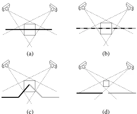
Figure 18: Pre-warped (a) and warped (b) voxel spaces shown in two dimensions. In (a), the voxel space is divided into two regions; an interior space shown with dark gray voxels, and an exterior space shown with light gray voxels. Both regions consist of voxels of uniform size. The warped voxel space is shown in (b). The warping does not affect the voxels in the interior space, while the voxels in the exterior space increase in size further from the interior space. The outer shell of voxels in (b) are warped to infinity. These voxels are represented with arrows in the figure.
4.1.1 Frustum Warp
We now describe a frustum warp function that is used to warp the exterior space. We develop the equations and fig-ures in two dimensions for simplicity; the idea easily ex-tends to three dimensions.
The frustum warp function presented here separates the voxel space into an interior space used to model foreground surfaces at fixed resolution, and an exterior space used to model background surfaces at variable resolution, as shown in Figure 18. The warping function does not af-fect the voxels in the interior space, while voxels in the exterior space are warped so that their size increases lin-early, in each dimension, with distance from the interior space. Under this construction, voxels in the exterior space will project to roughly the same number of pixels for view-points in or near the interior space. Voxels on the outer shell of the exterior space have coordinates warped to in-finity, and have infinite volume. While the voxels in the warped space have a variable size, the voxel space still has a regular 3D lattice topology.
The frustum warp assumes that both the interior space and the pre-warped exterior space have rectangular shaped outer boundaries, as shown in Figure 19. These bound-aries are used to define four trapezoidal regions,±x, and
±y, based on the region’s relative position to center of the interior space. These regions are also shown in Figure 19.
Let(x, y)be a pre-warped point in the exterior space, and let(xw, yw)be the point after warping. To warp(x, y),
Figure 19: Boundaries and regions. The outer boundaries of both the interior and exterior space are shown in the figure. The four trapezoidal regions,±xand±y are also shown.
we first apply a warping function based on the region in which the point is located. This warping function is applied only to one coordinate of(x, y). For example, suppose that the point is located in the+xregion. Points in the+xand
−xregions are warped using thex-warping function, xw=x
xe−xi
xe− |x|
,
wherexe is the distance along thex-axis from the center
of the interior space to the outer boundary of the exterior space, andxiis the distance along thex-axis from the
so the point does not move. However, points outside of the boundary get warped according to their proximity to the boundary of the exterior space. For a point on the bound-ary of the exterior space,x=xe, and soxw=∞.
(a)
(b)
Figure 20: Finding the warped point. Thex-warping func-tion is applied to the x-coordinate of the point(x, y), as the point is located in the+xregion. This yields the coordi-natexw, shown in (a). In (b), the other coordinateyw is
found by solving the line equation using the coordinatexw
found in (a).
Continuing with the above example, oncexw is
com-puted, we find the other coordinate yw by solving a line
equation,
yw=y+m(xw−x),
wheremis the slope of the line connecting the point(x, y)
with the point a, shown in (b) of Figure 20. Point a is located at the intersection of the line parallel to the x-axis and running through the center of the interior space, with the nearest linelthat connects a corner of the interior space with its corresponding matching corner of the exte-rior space, as shown in the figure. Note that in general, pointais not equal to the center of the interior space. By using such a construction, a point in a pre-warped region of space (e.g. +x) will stay in the that region after warping.
As shown above, the exterior space is divided into four trapezoidal regions for the two-dimensional case. In three dimensions, this generalizes to six frustum-shaped regions,
±x,±y,±z; hence the term frustum warp. There are three warping functions, namely thex-warping function as given above, andy- andz-warping functions,
yw = y
ye−yi
ye− |y|
zw = z
ze−zi
ze− |z|
.
In general, the procedure to warp a point in the pre-warped exterior space is as follows.
• Determine in which frustum-shaped region the point is located.
• Apply the appropriate warping function to one of the coordinates. If the point is the in±xregion, apply the x-warping function, if the point is in the±y region, apply they-warping function, and if the point is the
±zregion, apply thez-warping function.
• Find the other two coordinates by solving line equa-tions using the warped coordinate.
4.1.2 Resolution in the Exterior Space
The pre-warped exterior space is warped to infinity in all directions by the warping function, regardless of how many voxels are in the exterior space, assuming that the exterior space consists of a shell of voxels at least one voxel thick in each direction. However, the number of voxels in the ex-terior space determines the resolution of the exex-terior space. Adding more voxels allows finer details of distant objects to be more finely modeled.
4.2
Implementation Issues
Reconstruction and new view synthesis of a scene using a warped voxel space poses some challenges, which we now describe.
First, the warped voxel space extends to infinity in each dimension, and therefore cameras get embedded inside the voxel space. Since the photo-consistency measure is effec-tive only when each surface voxel is visible to two or more reference views, we must remove (pre-carve) a portion of the voxel space to produce a suitable initial surface for re-construction. User guided or heuristic methods can be used for pre-carving.
voxels. After reconstruction, if a new view is synthesized near such low resolution geometry, the resulting image will appear distorted, as large individual voxels will be identifi-able in the synthesized image. However, in our method, we intend for the reconstructed model to be viewed from in or near the interior space. For such viewpoints, objects in the exterior space will project to roughly a constant resolution that is matched to the outer shell of voxels in the interior space. This yields synthetic new views that do not suffer from such distortions.
4.3
Volumetric Warping Results
We have modified the GVC algorithm of Section 2 to utilize the warped voxel space. We performed a recon-struction using ten cylindrical panoramic photographs of a quadrangle at Stanford University. References [27, 41] discuss the calibration of such images. One of the 2500 x 884 photographs from the set is shown in Figure 21 (a). A voxel space of resolution 300 x 300 x 200 voxels, of which the inner 200 x 200 x 100 were interior voxels, was pre-carved manually by removing part of the voxel space con-taining the cameras. Then, the GVC algorithm was used to reconstruct the scene. A new synthesized view of the scene is shown in (b). Note that objects far away from the cameras, such as many of the buildings and trees, have been reconstructed with reasonable accuracy for new view synthesis.
Despite the successes of this reconstruction, it is not per-fect. The sky is very far away from the cameras (for prac-tical purposes, at infinity), and should therefore be repre-sented with voxels on the outer shell of the voxel space. However, since the sky is nearly textureless, cusping [39] occurs, resulting in protrusions in the sky. Reconstruc-tion of outdoor scenes is challenging, as surfaces often do not satisfy the Lambertian assumption made by our photo-consistency measure. On the whole, though, the recon-struction is accurate enought to produce convincing new views.
5
Conclusion
In this paper we have presented a collection of meth-ods for the volumetric reconstruction of visual scenes. These methods have been developed to increase the qual-ity, applicabilqual-ity, and usability of volumetric scene recon-struction. Visibility and photo-consistency are two es-sential aspects to any carving algorithm that reconstructs the photo hull. Accordingly, we introduced GVC, a full visibility reconstruction approach that supports arbi-trary camera placement and does not process inner vox-els. Our GVC-IB algorithm is memory efficient and eas-ily hardware accelerated, while our GVC-LDI algorithm
scenes. Our adaptive threshold method better reconstructs surface edges and texture, while our histogram intersec-tion method requires nearly no parameter tuning. Finally, we showed how the voxel space can be warped so that infinitely large scenes can be reconstructed using a finite number of voxels.
Volumetric scene reconstruction has made significant progress over the last few decades, and many techniques have been proposed and refined. Future work in this field may include more sophisticated handling of non-Lambertian scenes, new methods for reconstruction of time-varying scenes, and more computationally efficient methods for real-time reconstruction.
Acknowledgments
We thank Steve Seitz and Chuck Dyer for numerous dis-cussions regarding volumetric scene reconstruction. We are grateful to Mark Livingston and Irwin Sobel for cali-bration of the Stanford data set. We also express our grat-itude to Fred Kitson for his continued support and encour-agement of this research.
References
[1] Beardsley, P., Torr, P., and Zisserman, A. 1996. 3D Model Acquisition from Extended Image Sequences. In Proc. European Conference on Computer Vision, pp. 683 - 695.
[2] Bhotika, R, Fleet, D., and Kutulakos, K. 2002. A Prob-abilistic Theory of Occupancy and Emptiness. In Proc.
European Conference on Computer Vision Vol. 3, pp.
112 - 132.
[3] Blinn, J. and Newell, M. 1976. Texture and Reflection on Computer Generated Images. Communications of
ACM, 19(10): 542 - 547.
[4] Bolles, R., Baker, H., and Marimont, D. 1987. Epipolar-Plane Image Analysis: An Approach to De-termining Structure from Motion. In In International
Journal of Computer Vision 1(1): pp. 7 - 55.
[5] Broadhurst, A. and Cipolla, R. 2001. A Probabilistic Framework for Space Carving. In Proc. International
Conference on Computer Vision, pp. 388 - 393.
[6] Carceroni, R. and Kutulakos, K. 2001. Multi-View Scene Capture by Surfel Sampling: From Video Streams to Non-Rigid 3D Motion, Shape & Re-flectance. In Proc. International Conference on
(a)
(b)
Figure 21: Stanford scene. One of the ten reference views, (a), and reconstructed model projected to a new synthesized panoramic view (b).
[7] Chhabra, V., 2001. Reconstructing Specular Objects with Image-Based Rendering Using Color Caching. Master’s Thesis, Worchester Polytechnic Institute.
[8] Colosimo, A., Sarti, A., and Tubaro, S. 2001. Image-based Object Modeling: A Multi-Resolution Level-Set Approach. In Proc. International Conference on Image
Processing, Vol. 2, pp. 181 - 184.
[9] Culbertson, W. B., Malzbender, T., and Slabaugh, G. 1999. Generalized Voxel Coloring. In Proc. ICCV
Workshop, Vision Algorithms Theory and Practice,
Springer-Verlag Lecture Notes in Computer Science 1883, pp. 100 - 115.
[10] De Bonet, J. and Viola, P. 1999. Roxels: Responsi-bility Weighted 3D Volume Reconstruction. In Proc.
International Conference on Computer Vision, pp. 418
- 425.
[11] Debevec, P., Taylor, C., and Malik, J. 1996. Modeling and Rendering Architecture from Photographs: A Hy-brid Geometry and Image-Based Approach. In Proc.
SIGGRAPH, pp. 11 - 20.
[12] Dyer, C. 2001. Volumetric Scene Reconstruction from Multiple Views. In Davis, L. S. ed., Foundations of Image Analysis. Kluwer: Boston, MA, pp. 469 -489.
[13] Eisert, P., Steinbach, E., and Girod, B. 1999. Multi-Hypothesis, Volumetric Reconstruction of 3-D Objects From Multiple Calibrated Camera Views. In Proc. of
the International Conference on Acoustics, Speech, and Signal Processing, pp. 3509-3512.
[14] Eisert, P., Steinbach, E., and Girod, B. 2000. Auto-matic Reconstruction of 3-D Stationary Objects from Multiple Uncalibrated Camera Views. In IEEE Trans-actions on Circuits and Systems for Video Technology, 10(2), pp. 261 - 277.
[15] Faugeras, O. and Lustman, F., 1988. Motion and structure from motion in a piecewise-planar environ-ment. In Journal of Pattern Recognition and Artificial
Intelligence, 2(3) pp. 485 - 508.
[16] Faugeras, O. and Keriven, R. 1998. Complete Dense Stereovision Using Level Set Methods. IEEE
Transac-tions on Image Processing, 7(3): 336 - 344.
[17] Fua, P. and Leclerc, Y. 1995. Object-Centered Sur-face Reconstruction: Combining Multi-Image Stereo and Shading. International Journal of Computer
Vi-sion, 16(1): 35 - 56.
Graphics and Applications, pp. 21 - 29.
[20] Jebara, T., Azarbayejani, A., and Pentland, A. 1999. 3D structure from 2D motion. IEEE Signal Processing
Magazine, 16(3): 66 - 84.
[21] Johansson, B. 1999. View Synthesis and 3D Recon-struction of Piecewise Planar Scenes Using Intersec-tion Lines between the Planes. In Proc. InternaIntersec-tional
Conference on Computer Vision, 1999, Vol. 1, pp. 54
-59.
[22] Kimura, M., Satio, H., and Kanade, T. 1999. 3D Voxel Construction Based on Epipolar Geometry. In
Proc. International Conference on Image Processing,
pp. 135 - 139.
[23] Kutulakos, K. and Seitz, S. 1999. A Theory of Shape by Space Carving. In International Conference on
Computer Vision, Vol. 1, pp. 307 - 314.
[24] Kutulakos, K. and Seitz, S. 2000. A Theory of Shape by Space Carving. In International Journal of
Com-puter Vision, 38(3), pp. 199 - 218.
[25] Laurentini, A. 1994. The Visual Hull Concept for Silhouette-Based Image Understanding. IEEE
Trans-actions on Pattern Analysis and Machine Intelligence,
16(2): 150 - 162.
[26] Levoy, M. and Hanrahan, P. 1996. Light Field Ren-dering. In Proc. SIGGRAPH, pp. 31-42.
[27] Livingston, M. and Sobel, I. A New Scale Arbitration Algorithm for Image Sequences Applied to Cylindrical Photographs. HP Laboratories technical report HPL-2001-226R1, 2001.
[28] Longuet-Higgins, H., 1981. A Computer Algorithm for Reconstructing a Scene from Two Projections.
Na-ture, 293(10): 133 - 135.
[29] Matusik, W., Buehler, C., Raskar, R., Gortler, S., and McMillan, L. 2000. Image-Based Visual Hulls. In
Proc. SIGGRAPH, pp. 367 - 374.
[30] Max, N. 1996. Hierarchical Rendering of Trees from Precomputed Multi-Layer Z-Buffers. In Proc.
Euro-graphics Rendering Workshop, pp. 165 - 174.
[31] McMillan, M. and Bishop, G. 1995. Plenoptic Mod-eling: An Image-Based Rendering System. In Proc.
SIGGRAPH, pp. 39 - 46.
International Conference on Computer Vision.
[33] ¨Oz¨un, O. 2002. Comparison of Photo-Consistency Measures Used in the Voxel Coloring Algorithm. Mas-ters thesis, Middle East Technical University.
[34] Pfister, H. Zwicker, M. Van Baar, J., and Gross, M. 2000. Surfels: Surface Elements as Rendering Primi-tives. In Proc. SIGGRAPH, pp. 335 - 342.
[35] Pollefeys, M., Koch, R., Vergauwen, M., and Van Gool, L. 1999. Hand-Held Acquisition of 3D Models With a Video Camera. In Proc. 2nd International
Con-ference on 3-D Digital Imaging and Modeling, pp. 14
- 23.
[36] Prock, A. and Dyer, C. 1998. Towards Real-Time Voxel Coloring. In Proc. DARPA Image
Understand-ing Workshop, pp. 315 - 321.
[37] Saito, H. and Kanade, T. 1999. Shape Reconstruction in Projective Grid Space from Large Number of Im-ages. In Proc. CVPR, pp. 49 - 54.
[38] Savarese, S., Rushmeier, H., Bernardini, F., and Per-ona, P. 2001. Shadow Carving. In Proc. International
Conference on Computer Vision, Vol 1, pp. 190 - 197.
[39] Seitz, S. and Dyer, C. 1999. Photorealistic Scene Re-construction by Voxel Coloring. In International
Jour-nal of Computer Vision, 35(2): 151 - 173.
[40] Shade, J., Gortler, S., He, L., and Szeliski, R. 1998. Layered Depth Images. In Proc. SIGGRAPH, pp. 231-242.
[41] Shum, H. Y., Han, M., and Szeliski, R. 1998. Interac-tive Construction of 3D Models from Panoramic Mo-saics In Proc. CVPR, pp. 427 - 433.
[42] Slabaugh, G., Malzbender, T., and Culbertson, W. B. 2000. Volumetric Warping for Voxel Coloring on an Infinite Domain. In Proc. 3D Structure from Multiple
Images for Large Scale Environments (SMILE), pp. 41
- 50.
[43] Slabaugh, G., Culbertson, W. B., Malzbender, T., and Schafer, R. 2001. A Survey of Volumetric Scene Re-construction Methods from Photographs. In Proc.
International Workshop on Volume Graphics, pp. 81
-100.
[44] Slabaugh, G., Schafer, R., and Hans, M. 2002. Image-Based Photo Hulls. In Proc. 1st International
[45] Steinbach, E., Eisert, P., Betz, A., and Girod, B. 2000. 3-D Reconstruction of Real World Objects Using Ex-tended Voxels. In Proc. International Conference on
Image Processing, vol. I, pp. 569 - 572.
[46] Stevens, M., Culbertson, W. B., and Malzbender, T. 2002. A Histogram-Based Color Consistency Test for Voxel Coloring. In Proc. International Conference on
Pattern Recognition, vol. 4, p.118-21.
[47] Szeliski, R. 1993. Rapid Octree Construction from Image Sequences. Computer Vision, Graphics and
Im-age Processing: ImIm-age Understanding, 58(1): 23 - 32.
[48] Szeliski, R. and Golland, P. 1998. Stereo Matching with Transparency and Matting. In Proc. International
Conference on Computer Vision, pp. 517 - 524.
[49] Tsai, R. 1987. A Versatile Camera Calibration Tech-nique for High-Accuracy 3D Machine Vision Metrol-ogy Using Off-the-Shelf TV Cameras and Lenses.
IEEE Journal of Robotics and Automation, RA-3(4):
323 - 344.
[50] Vedula, S., Baker, S., Seitz, S., and Kanade, T. 2000. Shape and Motion Carving in 6D. In Proc. CVPR, Vol. 2, pp. 592 - 598.
[51] Weghorst, H., Hooper, G., and Greenberg, D. P. 1984. Improving Computational Methods for Ray Tracing.
ACM Transactions on Graphics, 3(1): 52 - 69.
[52] Yezzi, A. and Soatto, S., 2001. Stereoscopic Segmen-tation. In Proc. International Conference on Computer