Universit`
a degli Studi di Trento
PhD thesis
A tunable Bose-Einstein condensate for
quantum interferometry
Candidate:
Manuele Landini
Supervisor:
Prof. Giovanni Modugno
Supervisor:
Prof. Augusto Smerzi
Contents
1 Introduction 5
2 Theory 9
2.1 Laser and evaporative cooling . . . 9
2.1.1 Laser cooling . . . 10
2.1.2 Sub-Doppler cooling . . . 13
2.1.3 Evaporative cooling . . . 18
2.2 Bose-Einstein condensation . . . 20
2.2.1 BEC of weakly interacting atoms in a harmonic trap . . . 22
2.3 Tuning the interactions . . . 25
2.3.1 Square well potential . . . 28
2.3.2 Fano-Feshbach resonances . . . 31
3 Quantum interferometry 35 3.1 Two-mode atom interferometry . . . 35
3.1.1 Bloch sphere representation . . . 38
3.1.2 Entanglement and Fisher information . . . 42
4 Experimental apparatus 47 4.1 Experimental design . . . 48
4.3 Vacuum pumps . . . 50
4.4 Cooling laser system . . . 53
4.4.1 Laser locking . . . 56
4.4.2 Master-oscillator-power-amplifier . . . 58
4.4.3 High-power optical fibers . . . 60
4.5 Magnetic field coils . . . 61
4.6 Potassium samples . . . 65
4.7 2D-MOT . . . 67
4.8 3D-MOT . . . 69
4.9 Science chamber . . . 69
4.10 Magnetic transport . . . 71
4.11 Radio-frequency antennas . . . 72
4.12 Trapping lasers . . . 73
5 Sub-Doppler laser cooling 75 5.1 Laser cooling, the special case of potassium . . . 75
5.1.1 Cooling forces for a narrow hyperfine structure . . . 77
5.1.2 Sub-Doppler laser cooling of potassium . . . 82
5.2 Imaging techniques . . . 85
5.2.1 Fluorescence imaging . . . 85
5.2.2 Absorption imaging . . . 86
5.3 2D-MOT flux characterization . . . 87
5.4 3D-MOT operation and further cooling procedures . . . 88
5.4.1 3D-MOT loading from the atomic beam . . . 88
5.4.2 Compressed-MOT . . . 90
6 Bose-Einstein condensation of 39K 95
6.1 RF evaporation and Ramsauer-Townsend minimum . . . 99
6.2 Magnetic trap loading . . . 101
6.3 Transfer efficiency . . . 104
6.4 Dipole trap loading from magnetic trap . . . 108
6.4.1 Light induced losses . . . 110
6.4.2 Feshbach resonances and field calibration . . . 111
6.5 All-optical evaporation of the atomic sample . . . 112
6.6 A tunable Bose-Einstein condensate . . . 114
7 Towards quantum interferometry 119 7.1 Thermal effects on the coherence of a BEC in a double well . . . 119
7.1.1 Theoretical modeling . . . 120
7.1.2 Parameter regions . . . 122
7.1.3 Classical results . . . 123
7.1.4 Quantum results . . . 124
7.2 Optical double well design . . . 127
7.3 Detection issues and possible strategies . . . 131
Chapter 1
Introduction
Since the first experimental realization of a Bose-Einstein condensate (BEC) in
1995[1], increasing interest has grown around these particular objects. The principal
reason is that BECs are macroscopic, therefore easily observable, but their behavior
is completely dominated by their wave nature. Thanks to this property a lot of
exciting research was carried out using BECs, spanning many different research
fields[2]. For example the observation of their superfluid behavior, the most striking
evidence being the formation of quantized vortices[3], has led to test various theories
developed in the context of superfluid Helium. BECs can be also used to simulate
interesting phenomena of condensed matter physics like Andersson localization[4,
5], the superfluid to Mott insulator transition[6] and many others. Recently the
achievement of single atom and single site resolution in such systems opens a new era
of observations in this direction[7]. BECs in optical lattice represents also appealing
candidates for quantum computation[8] thanks to their long coherence times, good
scalability, and the control of interactions between atoms via Feshbach resonances[9,
10, 11].
The subject of this thesis is the use of BECs for atom interferometry[12, 13].
falling samples of atoms[14]. The employed samples are cold (but not condensed)
to have high coherence, and dilute, not to interact significantly with each other.
This technique represents nowadays an almost mature field of research in which the
achievable interferometric sensitivity is bounded by the atomic shot noise. Until
a few years ago the employment of BECs in such devices was strongly limited by
the effect of the interactions between the condensed atoms. This obstacle is today
removable exploiting interaction tuning techniques. The use of BECs would be
ad-vantageous for atom interferometry inasmuch they represents the matter analogue
of the optical laser providing the maximum coherence allowed by quantum
me-chanics. In this direction, enhanced phase coherence was demonstrated employing
almost non-interacting samples[15]. Moreover, non-linear dynamic can be exploited
in order to prepare entangled states of the system. The realization of entangled
samples can lead to sub-shot noise sensitivity of the interferometers[16]. At today
very nice proof-of-principle experiments have been realized in this direction[17, 18]
but a competitive device is still missing.
This thesis work is inserted in a long term project whose goal is the realization of
such a device. The basic operational idea of the project starts with the preparation
of a BEC in a double well potential. By the effect of strong interactions the atomic
system can be driven into an entangled state. Once the entangled state is prepared,
interactions can be ”switched off” and the interferometric sequence performed. The
two modes of the interferometer that we want to build will be represented by the two
ground states of two spatially separated potential wells created via optical potentials.
The measured phase will be sensitive to the energy difference between the wells. The
use of a trapped configuration would also allow for very long phase accumulations
as compared to a free-falling scheme.
This thesis begins with the description of the apparatus for the production of
because this atomic species presents many convenient Feshabch resonances at
eas-ily accessible magnetic field values. The cooling of this particular atomic species
presents many difficulties, both for the laser and evaporative cooling processes.
For this reason, this was the last alkaline atom to be condensed. Its
condensa-tion up to now was only possible by employing sympathetic cooling with another
species[19, 20]. In this thesis our solutions to the various cooling issues is reported.
In particular we realized sub-Doppler cooling for the first time for this species and
we achieved condensation via evaporation in an optical dipole trap taking
advan-tage of a Feshbach resonance. In the last part of this work, are presented original
calculations for the effects of thermal fluctuations on the coherence of a BEC in a
double well, discussing the interplay between thermal fluctuations and interactions
in this system. Estimations and feasibility studies regarding the double well trap to
be realized are also reported. This kind of calculations are part of the design process
in order to identify realistic operational parameters and optimized design strategies
for the realization of the double well interferometer.
In more details, Chapter 2 contains an introduction to the theory of atomic
cooling (laser cooling and evaporative cooling). In Chapter 3 are revised the basic
aspects of quantum interferometry. The details about the building and operation
of the experimental apparatus are given in Chapter 4. The achievement of
sub-Doppler cooling and the details of the laser cooling procedures are the subject of
Chapter 5. The optimization of the optical and magnetic trapping techniques, as
well as the achievement of condensation in single species operation are reported in
Chapter 6. In Chapter 7 are given the theoretical calculations about thermal effects
on the condensate coherence together with calculations regarding the realization of
Chapter 2
Theory
Here I give the basic theoretical background for the physical phenomena explored
in this thesis. Sec.2.1 of the chapter describes the cooling techniques used to cool
a thermal gas of atoms to the extremely low temperatures that are necessary to
achieve Bose-Einstein condensation (BEC). Sec.2.2 recalls the principal features of
this quantum state of matter. In Sec.2.3 is described the tool of Fano-Feshbach
res-onances, used to control the atomic interactions in the BEC. In Sec.2.4 is introduced
the theoretical framework for the description of a double well Mach-Zehnder atomic
interferometer.
2.1
Laser and evaporative cooling
The two basic techniques used to reach low temperatures in alkaline’s atomic gases
are laser cooling and evaporative cooling. Laser cooling allows to cool a gas from
2.1.1
Laser cooling
In the description of laser cooling I am going to make use of the semi-classical
picture for the atomic interaction with the light field[21]. In doing this, I will treat
the internal degrees of freedom of the atom in a fully quantum mechanical way. The
external degrees of freedom (position and momentum), as well as the light field, will
instead be treated classically. To do so one has to be sure that the atomic position
and velocity are well defined during the interaction with light
∆x≪λ (2.1)
k∆v ≪Γ . (2.2)
Here ∆x is the spatial extension of the atomic wavepacket, which is given by the De Broglie wavelength; λ is the wavelength of the laser light, and k=2π/λ is the wavenumber. ∆v is the velocity spreading of the atomic wavepacket. Γ is the scattering rate which is given by Γ=2π/τ, withτ the radiative lifetime of the excited atomic level. By writing the Heisenberg indetermination principle for the conjugated
variables of the atomic motion and making use of the above equations the following
condition can be obtained:
ER=
~2k2
2m ≪~Γ (2.3)
in which ~=h/2π with h the Planck constant.
The quantity on the left-hand-side is the recoil energy that an atom gets from the
light field in an absorption event. This is also called the broadband condition[22].
It ensures that the interaction with the light field does not change significantly the
atomic energy. If 2.3 is verified the atomic conditions don’t change significantly
over many absorption re-emission cycles. For the cooling transition of39K the ratio
~Γ/ER is about 350.
Under this condition it makes sense to consider the mean optical dipole force
Given the electric fieldE generated by a monochromatic laser beam of polarization
unit vectorbǫ, field amplitude E, angular frequency ωL=2πc/λ and phase φ:
E=bǫ(x)E(x) 2 e
−i(ωLt−φ(x))+c.c. . (2.4) The mean force the light field exerts on an atom is:
F= X
i=x,y,z
di∇Ei . (2.5)
Hered is the averaged atomic dipole operator:
d=hDi=T r(ρatD) , (2.6)
ρat is the steady-state atomic-density operator, given by the solution of the optical
Bloch equations (OBE)[23].
In the simple case of a two-level atom at rest, the expression for the force has
two contributions: the radiation pressure force and the dipole force
FRP =
~Γ
2
s
1 +s∇φ , (2.7)
Fdip =−~δ 2
∇s
1 +s . (2.8)
Here δ=ωL-ωA is the detuning from the atomic transition and s is the saturation
parameter
s= Ω 2/2
δ2+ Γ2/4 (2.9) Ω=Ed0bǫ/~is the Rabi frequency andd0 is the matrix element of the dipole operator between the ground- and the excited-state electronic wavefunctions.
Let us discuss the effect of these two forces. For the case of a single plane wave
(φ(x) =kx and s=const) the dipole force is zero and the radiation pressure is:
FRP =~k
Γ 2
s
1 +s (2.10)
this force can be interpreted as the viscous force coming from scattering of photons
the spontaneously re-emitted photon takes off in a random direction, not changing,
on average, the atomic momentum. The acceleration that this force can cause on a
potassium atom fors ≫1 is 2.4×10⁵m/s2, which is sufficient to stop an atom moving at 250 m/s (typical velocity for an atom at room temperature) over a distance of
12 cm in a ms.
To have a non zero dipolar force, it is necessary to allow a spatial variation of
the beam amplitude, or, in other words, one needs to deal with several plane waves.
The dipolar force is originated by the redistribution of photons that an atom can
operate by absorbing a photon from one plane wave and emitting it by stimulated
emission in another one. The dipolar force can be derived from a potential
Udip =
~δ
2 ln(1 +s(x)) , (2.11) it is thus conservative and it can be used for trapping. The dipole potential is
related to the light shift or AC Stark shift ∆AC by Udip = ~∆AC. In the limit of
low saturation (s≪1) there is a simple relation between scattering rate and dipole potential
γ = Γ
~δUdip = Γ
δ∆AC . (2.12)
The modification to the force, caused by the fact that the atom is in movement
with velocity v, only consists in considering the laser frequency as seen by the
atom. The Doppler effect modifies the laser frequency according to: ω′
L = ωL
-kv, δ′=δ-kv. Let us consider the situation in which the atoms interact with two counterpropagating plane waves. In this case, by Taylor expanding the radiation
pressure force for the two laser fields at small velocity, one gets:
F=−αv . (2.13)
In the case of low saturation, the contributions from the two plane waves can be
added independently and the value of the friction coefficient is:
α=−~k2s 2δΓ
If δ < 0, this force causes dissipation. The velocity range over which the Taylor expansion remains valid (velocity capture range) is given by v<Γ/k, that is satisfied if the semi-classical picture is applicable.
Spontaneous emission does not change the mean velocity, but can change the
averaged square velocity by causing fluctuations. Fluctuations are described by a
random walk in momentum space, expressed by
hp2i(t) = 2Dpt . (2.15)
By the fluctuation-dissipation theorem, the limit temperature reachable by laser
cooling is as follows
kBT =
Dp
α . (2.16)
The calculation of the diffusion constant for a two-level system gives Dp =~2k2Γs.
This cooling scheme is called an ”optical molasses”[24] and is applicable also in 3D.
The temperature one gets for a two level atom is called Doppler temperature. It is
independent of the laser power and it is minimum for δ=−Γ/2, for which its value is given by:
kBTD =
~Γ
2 . (2.17)
For the D2 transition used for cooling potassium TD ≃145 µK.
2.1.2
Sub-Doppler cooling
Cooling below the Doppler temperature is possible for multilevel atoms in presence
of a non homogeneous polarization of the light field[25]. To get some insight, we
can consider the electric field generated in a common experimental situation. Let us
take two counter-propagating laser fields of opposite circular polarization (σ−for the beam propagating alongzandσ+ for the one propagating in the opposite direction). The resulting electric field is always linearly polarized with the polarization axis that
Figure 2.1: Polarization pattern produced by the laser configuration described in
the text, the resulting electric field has linear polarization, the polarization axis
describes an helix with step λ
along z it will therefore see the light polarization rotated by an anglekz.
The simpler transition exhibiting sub-Doppler cooling in this situation is a J = 1 → J′ = 2 transition. If we take as the quantization axis z, and we analyze the situation for an atom at rest at in a given position, for which the polarization of
the light is bx, it is possible to calculate the light shifts and the populations of the different ground state sub-levels. The result is, of course, symmetric for mF = +1
and mF =−1. If we repeat the analysis for an atom at rest in another position and
with a different polarization of the light, nothing will change. So the light shifts
and the populations in the ground state are independent of position for an atom at
rest. If we now consider an atom moving in such a laser configuration with velocity
during its motion or not.
We will work in a regime of velocity such that kv ≪ Γ in order to neglect the Doppler effect on detuning. The simplest approach is to describe the system in a
rotating reference frame in which the laser polarization is constant. In this reference
frame, a non inertial term is added to the Hamiltonian
Vrot=kvJz . (2.18)
This term rises the energy of the mF = +1 state and lowers the energy of the
mF =−1, causing an imbalance in the populations of these two levels due to optical
pumping processes. To calculate such imbalance one has to solve the OBE of the
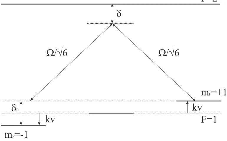
system. To have an estimation of the imbalance, we can consider the coherent
Raman process that couples the mF = 1 state to the mF =−1 through absorption
of a photon from the σ− beam and re-emission into the σ+ one (see Fig.2.2). We
F=2
F=1
d
W/Ö6
W/Ö6
m =+1
Fm =-1
Fkv
kv
d
RFigure 2.2: Scheme of the Raman coupling described in the text.
dependence even forkv ≪Γ. We can restrict the analysis to the two levels coupled by the Raman transition and describe the process on the Bloch sphere. The effective
Rabi frequency of the Raman coupling is
ΩR=
Ω2/6
δ , (2.19)
the effective detuning of the Raman transition is
δR = 2kv . (2.20)
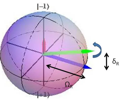
The situation is the one depicted in Fig.2.3. Forv = 0 there is no evolution, and the populations remain balanced. The introduction of a Raman detuning by the atomic
velocity gives rise to a Rabi oscillation around the combined axis. On average and
for small angles the population imbalancep will be
p≈ δR
ΩR
= 2kvδ
Ω2 (2.21)
in favor of the mF=-1 state for positive δ. It is easy to see that, for increasing
Raman detuning, the imbalance reaches a maximum for kvc ≈ Ω2/δ; this defines
the velocity capture range of sub-Doppler cooling. The force generated by the
population imbalance is simply the radiation pressure force times p(theσ− beam is pointing towards the velocity).
FSD ≈~k
Γ 2sp≈
~k2δΓ
δ2 + Γ2/4v (2.22) which gives, for the friction coefficient at large detuning:
αSD ≈ −~k2
Γ
δ . (2.23)
Remarkably this is independent of laser power. The pre-factor on the above
estima-tion and possible deviaestima-tions from this behavior at small detuning will depend on the
particular level scheme that one is dealing with. It is easy to see that the population
Figure 2.3: Bloch sphere representation of the effect of the Raman coupling. The
situation in which ΩR (and since δ) is positive is shown, in this case, on average
there are more atoms in the mF =−1 level. The initial situation is supposed to be
with the representative Bloch vector aligned with ΩR for simplicity.
state δR ∝ m, with m the magnetic quantum number. So an higher degeneracy
implies higher friction. For large detuning,δ ≫Γ, using the same diffusion constant in momentum space used for the Doppler case, one gets:
kBTSD =
Dp
αSD ≈
~Ω2
δ ≈kBTD I Is
Γ
δ (2.24)
in which we made use of Ω = Γ2q2IIs. I is the intensity of the light wave and Is is
the saturation intensity.
From the above expression one sees that, using this method it is possible to reach
very low temperatures. Forδ ≫Γ andI ≪Is, the temperature can be much lower
than the Doppler temperature. The limit of the cooling method is reached when the
thermal velocity spread exceeds the velocity capture range of the process. At that
reaching TD. For the limit temperature:
kBTlim ≈
1 2mv
2
c ≈
m
2~2k2 ~2Ω4
δ2 ≈
k2
BTlim2
ER
; (2.25)
this implies
kBTlim ≈ER . (2.26)
In conclusion, this cooling method is limited only by the recoil energy, which for
potassium is 0.4 µK. The prefactor on the expression for the limit temperature was calculated using Monte Carlo simulations and was found to be in the range of 10-40,
depending on the actual level scheme[26].
2.1.3
Evaporative cooling
In order to reach even lower temperatures, an evaporative cooling scheme is used by
which the higher energy atoms are selectively extracted from the trap. The atoms
with higher energy are populating the low density tails of the cloud. If they are
removed slowly, on a time scale which is longer than the time the cloud needs to reach
thermal equilibrium τeq, the evaporation determines cooling and the process can be
sustained up to the condensation point. Since only a few collisions are sufficient
to equilibrate the thermal distribution, we can approximate τeq ≃ τcoll = (nσv)−1,
in which σ is the cross section for elastic collisions between atoms, n is the atomic density, and v the typical atomic velocity. This is indeed the same process that happens everyday when a cup of coffee cools down.
In cold atoms this process is usually realized in magnetic or optical traps. In a
magnetic trap, the spatial variation of the magnetic field across the trap offers an
elegant way to evaporate the cloud. Using a radio frequency transition, the trapped
state can be coupled to an untrapped one. The frequency can be chosen in such a
removes all atoms on a ”resonance surface” (three dimensional evaporation). The
radio frequency gets progressively reduced up to the condensation point.
In an optical trap instead, a focused laser beam, tuned on the red of the atomic
transition, is used for trapping by the dipole potential. The potential experienced
by the atoms is given by:
U(x) =α(ωL)I(x) = α(ωL)
I0 1− z2
z2 0
e−
2r2
W02 (2.27)
where α(ωL) is the atomic polarizability at the laser frequency, I0 is the intensity at the focal point, z and r are coordinates along and transverse to the laser beam axis respectively, W0 is the beam waist, and z0 = πW02/λL is the Rayleigh range.
This potential yields a finite depth given by U0 =α(ωL)I0. Atoms with an energy larger thanU0 cannot be confined by the potential and they will leave the trap due to gravity. Atoms are therefore lost on a preferential direction (one dimensional
evaporation). The evaporation in this case is performed by progressively reducing
the laser power and therefore the trap depth. Differently from the magnetic case,
for dipole traps, during evaporation the trap frequencies are also reduced. This can
be a problem since it causes the collision rate to decrease in typical situations.
The first quantity that characterizes the evaporation is the truncation
param-eter η = U0/(kBT). A low η inhibits thermalization, while a high one results in
slow evaporation, that can in turn lead to losses. The evaporation rate, in fact,
is determined by the truncation parameter. Every time a collision takes place, the
probability to evaporate a new atom is given by the Boltzmann factore−η. Therefore
for the evaporation rate:
Γev = Γele−η (2.28)
with
Γel =
1
τcoll
=nσv (2.29)
ramp, determining the optimum value of the truncation parameter. The first one
is the thermalization time τeq that is the inverse of the elastic collision rate. The
second time scale is determined by losses and heating in the system; these can
be of various nature: collisions with the background gas, two-body or three-body
collisions, technical noise on the trapping potential, etcetera. They all contribute to
an inelastic rate Γin. The evaporation is efficient when the evaporation rate is, on
the one hand, lower than the elastic collision rate (necessary condition for the gas
to be able to equilibrate), and on the other, higher than the inelastic collision rate
(condition this for the evaporation to be the dominant loss process). This means
that a lower η is favorable when we are in presence of strong inelastic rates. There is anyway a limit. In fact it can be proven that, for a harmonic trap, an η <3 leads to a decreasing phase space density during the evaporation[27].
The efficiency of the evaporation process is measured by the χparameter, which is defined by:
χ= logρf/ρi logNi/Nf
(2.30)
in which ρi(f) is the initial (final) phase space density andNi(f) is the initial (final)
number of atoms.
2.2
Bose-Einstein condensation
Bose-Einstein condensation is a phase transition occurring when the thermal De
Broglie wavelength λDB of the particles
λDB =
h
√
2πmkBT
(2.31)
becomes comparable with their inter-atomic distance[28, 29]. In this regime the
wave nature of atoms becomes dominant and quantum effects are important for the
macroscopic behavior of the system. In terms of the phase space density
the phase transition takes place when ρ=2.612.
For a normal gas at room temperature and atmospheric pressure the De Broglie
wavelength of the particles is smaller than the atomic radius, the phase space density
of the gas is around 10−7. From this point, it is possible to increase the phase space
density either by increasing the density or decreasing the temperature. However,
as can be seen from Fig.2.4, the BEC transition happens in a region of the phase
diagram in which the equilibrium state of matter is a solid1.
Figure 2.4: Phase diagram of a typical bosonic element. The BEC region is dashed
since the true equilibrium state of the system is the solid state.
This means that all BECs are metastable, the solid state being the true ground
state of the system. The first processes that leads to the sample’s solidification are
the ones in which three atoms collide, two of them form a molecule and the third
one ensures conservation of momentum. The binding energy of the molecule gets
converted into kinetic energy, leading to the loss of all three atoms from the trap
(three body loss). If the sample is dilute the probability to find three atoms, close
enough to determine a three body loss, can be negligible and the lifetime of the
BEC can be long. To be quantitative, three body losses in a gas are described by
the formula
˙
n =−K3n3 (2.33) The minimum value of K3 for 39K is 10−29 cm6/s. For a normal BEC at a density of 1014 atoms/cm3, this equation predicts a 10 s lifetime for the condensate. Such
density is 5 orders of magnitude lower than the density of air at atmospheric pressure.
2.2.1
BEC of weakly interacting atoms in a harmonic trap
In experiments, we deal with interacting samples of atoms trapped by
inhomoge-neous external potentials. To describe the system in this situation the so-called
Gross-Pitaevskii equation[30] (GPE) is required. In second quantization, the
many-body Hamiltonian operator describing a system ofN bosons in an external potential
Vext is given by
b
H =
Z
dxΨb†(x)
−~
2∇2
2m +Vext(x)
b
Ψ(x)+
1 2
Z Z
dxdx′Ψb†(x)Ψb†(x′)Vint(x,x′)Ψ(b x)Ψ(b x′) . (2.34)
In the case of ultra-cold bosons, the interaction potential can be greatly simplified.
Every collision channel but the s-wave is in fact strongly inhibited due to the very low collisional energy (see Sec. 2.3). When only s-wave scattering is present, the details of the interaction potential are not important anymore, therefore it can be
substituted by a pseudo-potential with the same s-wave scattering amplitude
Vint(|x−x′|)→
4π~2a
m δ(x−x
Even with this simplification, the solution of the Schr¨odinger equation for a sys-tem of typically 105 atoms is a numerically impracticable task. To further simplify
the problem, we can make use of our knowledge of the ground state of the
sys-tem. The ground state is the condensate, which is characterized by a macroscopic
occupation of a single quantum state. In this case, the fluctuations on the wave
function amplitude can be neglected and the amplitude itself can be substituted by
a c-number (mean field approximation)[31]:
b
Ψ(x) =bb0Ψ0(x) +δΨ(b x)≈pN0Ψ0(x) . (2.36) Here bb0 is the destruction operator of the ground state, Ψ0(x) is the condensate wave-function, and δΨ(b x) represent excitations of the system, which are neglected.
N0 is the number of atoms in the ground state. By substituting this ansatz for the wave-function back into the Hamiltonian and writing the equation of motion, we get
the GPE
i~Ψ0(˙ x, t) =
−~
2∇2
2m +Vext(x) +
4π~2a
m |Ψ0(x, t)|
2
Ψ0(x, t) . (2.37) From the mathematical point of view the GPE is a single particle Schr¨odinger equa-tion with a non-linear term accounting for interacequa-tions. The staequa-tionary soluequa-tion to
this equation is calculated by replacing Ψ0(x, t) = e−iµt/~
Ψ0(x)
µΨ0(x) =
−~
2∇2
2m +Vext+
4π~2a
m |Ψ0(x)|
2
Ψ0(x) (2.38)
the parameter µis the chemical potential of the condensate.
This equation has two limit behaviors: for very low interaction strengths the
non linear term can be neglected and the GPE becomes simply the Schr¨odinger equation for a particle in the external potential Vext. In this case the condensate
wavefunction is nothing but the ground state wavefunction of a single particle in the
external potential. If the potential is harmonic with angular frequenciesωx, ωy, ωz
Ψ0(x, y, z) =
mω π~
3/4
here ω is the geometric average of the three angular frequencies. The chemical potential in this case is simply the harmonic oscillator ground state energy µ =
~(ωx+ωy+ωz)
2 .
The other limit case is the one in which repulsive interactions are dominating
over the kinetic term. In this case, which is the case for typical BECs, we can neglect
the kinetic term in the GPE applying the so-called Thomas-Fermi approximation. In
this case, the GPE becomes a simple algebraic equation for the condensate density,
whose solution gives an inverted parabola profile of the condensate
n(x, y, z) = |Ψ0(x, y, z)|2 = m
4π~2a(µ−Vext(x, y, z))θ(µ−Vext(x, y, z)) . (2.40) The chemical potential is obtained by the condition that the integral ofn gives the total atom number and it is given by
µ= ~ω 2
15N a lho
2/5
, (2.41)
where lho is the harmonic oscillator length. For the same potential considered in
the non interacting case, the density at the center and the radii of the cloud can be
calculated
n0 =
m
4π~2aµ (2.42)
Ri =
s
2µ mω2
i
(2.43)
fori=x, y, z. The condition for the interaction energy to be larger than the kinetic energy can be rephrased in µ≫ ~ω/2[32]. This is true if N a ≫lho. The oscillator lengthlho for a typical trapping frequency of 100 Hz is 1.6 µm. For a condensate of
105 atoms, N a become 10 times larger than l
ho for a scattering length of only 3 a0,
2.3
Tuning the interactions
Interactions among neutral atoms are typically due, on the one hand, to Fermi
pressure at short distances which prevents the nuclei to come too close to each
other, and on the other, to Van Der Waals attraction at large distances, which fall
off with the interaction distance r as r−6. To treat collisions I will make use of some well known results from scattering theory[33]. Before going into details, let
us consider the typical length scales in the system. The three relevant distances for
the collisional physics of the gas are: the inter-particle distance n−1/3, the range of action of the interaction potential r0, and the De Broglie wavelengthλDB. Since we
deal with dilute gases n−1/3 > r
0, is typically valid. At high temperature, the De
Broglie wavelength is shorter than r0 . Decreasing the temperature, λDB becomes
of the same order, or larger, than r0. Finally, for even lower temperatures, it can reach n−1/3 leading to condensation. In the intermediate regime,r
0 < λDB < n−1/3,
the gas is still thermal but the wave nature of the particles influences the collisional
properties. A quantum-mechanical treatment of the collisions is therefore required.
To have an idea, if we consider an r0 of around 2-3 nm, the De Broglie wavelength is larger thanr0 for temperatures lower than 10 mK.
Let us consider the collision of two atoms having the same mass m. The full Hamiltonian reads
H = |p1| 2
2m +
|p2|2
2m +V(|r1−r2|) . (2.44)
The interaction potential is supposed to have central symmetry, since we will always
deal with alkali atoms with one unpaired electron in the external s orbital. We can introduce the center of mass and relative coordinates, in which the Hamiltonian is
re-written as
H = |pCM| 2
4m +
|p|2
the following notations are used
p1+p2 =pCM =~kCM, p1−p2
2 =p=~k, (2.46)
r1+r2
2 =rCM, r1−r2 =r . (2.47) It is a known result of scattering theory that for the system wave-function after the
collision the following limit behavior is valid
Ψ(r1,r2)→r→∞ eikCM·rCM
eik·r+fk(θ)
eik|r|
|r|
. (2.48) where θ is the axial angle between r and k. This equation consists of two terms in the relative reference frame: the first one describes the two waves passing away
from each other (transmission), while the second one describes a spherical wave
originated from the collision point (diffusion). The quantity f(θ) sets the strength of the diffusion with respect to the transmission and it can only depend on the axial
angle because of the cylindrical symmetry of the problem.
The above expression needs to be symmetrized (bosons) or anti-symmetrized
(fermions) if we are dealing with identical particles. The only term that changes
when exchanging the two particles is f(θ). It is easy to realize that the two events depicted in Fig.2.5 are indistinguishable for identical particles. The symmetrization,
Figure 2.5: The two collisional events in this picture are indistinguishable for
therefore, consists simply in the replacement
f(θ)→f(θ)±f(π−θ) (2.49) with the plus sign for bosons and the minus sign for fermions. The total cross section
for the collision process can be found to be
σtot = 2π
Z π 2
0 |
f(θ)±f(π−θ)|2sin(θ)dθ . (2.50) Since the interaction potential is centrally symmetric we can describe the collision
in term of partial waves. The symmetrization causes the cancellation of the odd
waves for bosons and of the even ones for fermions
σtot =
8π k2
X
2l
(2l+ 1) sin2(δl(k)) (bosons) (2.51)
σtot =
8π k2
X
2l+1
(2l+ 1) sin2(δl(k)) (f ermions) (2.52)
The parametersδl(k) are the partial wave’s phases and they carry information about
the interaction potential. The equation for the radial wave function uk,l is
u′′k,l(r) +
k2+ l(l+ 1)
r2 +V(r)
uk,l(r) = 0 . (2.53)
This equation is the same as the one describing the 1D motion of a particle moving
in the effective potential Vef f(r) = l(lr+1)2 +V(r). The potential V(r) has a typical range of action of a few nm, while for larger distances the repulsive centrifugal term
dominates.
If V(r) = 0, the shortest distance a particle with low energy can reach is rl =
√
l(l+1)
k , which is of the order of the De Broglie wavelength (λDB ≈ 1/k). At the
condensation point, the De Broglie wavelength can take typical values of about
1 µm; therefore, unless l = 0, the potential is unreachable by the particles. This phenomenon can be visualized in terms of a centrifugal barrier given by the term
l(l+1)
centrifugal barrier’s height, the only partial wave contributing to the scattering is
the s-wave. Because of this and of the symmetrization rules, it follows that ultra-cold fermions are practically non-interacting and that the cross section for bosons
is
σtot =
8π k2 sin
2(δ0(k)) . (2.54) At this point we can define thes-wave scattering length to be
a= lim
k→0−
δ0(k)
k , (2.55)
such that
lim
k→0σtot = 8πa
2 . (2.56)
The only parameter that we need to know, in order to characterize the collision at
low energy is thus a.
2.3.1
Square well potential
To get some insight on the scattering length, we can look at the simple case in which
the interaction potential is a square well. For this potential, the scattering problem
is easily solvable analytically.
V =−V0 0< r < r0
V = 0 r0 < r < R
V =∞ r > R
(2.57)
here I also inserted a finite system size R, which is supposed to be larger than any other length scale of the problem.
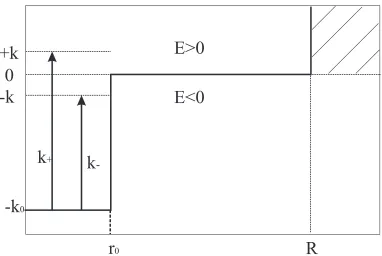
Let us start by considering the continuum states for E > 0 and l = 0. The equation for the radial wave function can be solved in the different zones, giving
u0 =Asin(k+r) 0< r < r0
u0 =Bsin(kr+δ0) r0 < r < R
u0 = 0 r > R
r
0R
-k
0k
-k
++k
-k
0
E>0
E<0
Figure 2.6: Square well potential with the related notations
wherek=√2mE/~,k0 =√2mV0/~, and k2
+ =k02+k2. By imposing the continuity of the wavefunction inR, we get
sin(kR−δ0)→k→0 sin(k(R−a)) = 0 . (2.59) The limit follows from the very definition of a. This implies the quantization of k
by
kn =
nπ
R−a . (2.60)
If the interaction potential was not present, the previous expression with a = 0 would have given the energy of one particle in the box with size R. The presence of the second particle changes the energy, increasing it for positive a (repulsion) and decreasing it for negative a (attraction). Now we impose the continuity of the logarithmic derivative of the wave-function atr0:
Solving for k≈0, the following equation can be found for the behavior of the phase
δ0 at non-zero energy[34]
tan(δ0)
k ≈ −a−
1 2a
2r
ek2 . (2.62)
The parameter re is the effective radius that, in the case of a square well potential,
is approximately equal to r0. Since the second term has a fixed sign, when the scattering length is found to be negative and small, a zero in the phase δ0 is pre-dicted for low energy 2. This is the so-called Ramsauer-Townsend effect[35], which
represents a serious issue when evaporatively cooling some atomic species (85Rb and
39K are two examples). Indeed, when the typical energy of the cloud approaches the
Ramsauer-Townsend minimum, the system is no more able to thermalize and the
evaporation becomes inefficient or stops completely. Let us go back to the continuity
equation 2.61, fork = 0 it reads 1
r0−a
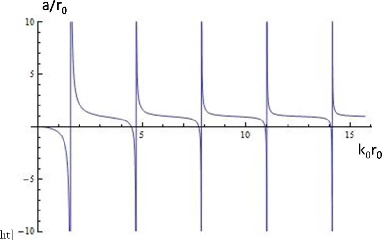
=k0cot(k0r0) . (2.63) Solving it for a, we get
a=r0−
tan(k0r0)
k0
. (2.64)
A plot of this formula is on Fig.2.7: a divergence in the scattering length is predicted
each timek0r0 = π2 +nπ.
To get some more insight we can consider the same problem but now for a very
shallow bound state (E <0). The solution to the radial wave equation, in this case,
is:
u0 =Asin(k−r) 0< r < r0
u0 =Be−kr r0 < r < R
u0 = 0 r > R .
2Actually, the expansion of the phase in series of k is no more appropriate at the position of
the zero. Nevertheless, more accurate calculations still predicts its presence. Its position cannot
[ht]
Figure 2.7: Scattering length in units of r0 as a function of the parameter k0r0. A resonant behavior is apparent every time a new bound state is added to the potential.
The continuity of the logarithmic derivative of the wavefunction in r0 leads to
−k =k0cot(k0r0) . (2.65) In the limit of a very shallow bound state, k →0, the condition of Eq.2.65 has to connect to the one for E >0, Eq.2.63. This is only possible if a diverges. This means that, each time a new bound state is added to the potential, the scattering
length shows a divergence. When the bound state is about to show up,ais negative and large. When instead it is just appeared, a is positive and large.
2.3.2
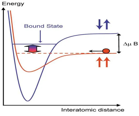
Fano-Feshbach resonances
The simple picture, given by the analysis of the square well potential, applies also
in practical situations, in which many molecular adiabatic potentials are present.
behavior is found in the scattering length any time a new bound state is added
to the interatomic potential. In practice, a new bound state can be added to the
potential exploiting the presence of many different interatoimic potential curves due
to collision into different spin channels. For large distances, those curves connect to
the sum of the energies of the free colliding atoms. Such energies have a magnetic
component that can be changed by applying an external magnetic field. Doing so,
two of these potential curves can be shifted in energy with respect to each other (see
Fig.2.8). Due to residual interactions (spin orbit couplings, dipolar interactions,
etc.), the two potential curves are not completely independent. For this reason,
whenever a bound state of one of the potentials is close to the dissociation threshold
of the potential in which the collision takes place, the scattering length shows a
resonant behavior.
Figure 2.8: Sketch of the basic principle of a Feshbach resonance.
Those resonances are named Fano-Feshbach resonances and they are used in
experiments to have control over the inter-atomic interaction, simply applying a
the lab can be of the order of a few tens of mG and, therefore, tuning the interactions
on sharp resonances can be challenging. The resonances, in exceptional situations
(experimentally identified for39K,6Li,7Li, Na, Cs), can be as wide as 10-100 G and
they can take place at easily accessible values of the magnetic field. To understand
what can lead to wide resonances, we can consider the coupling between the two
states involved in the process. The initial state is a continuum state, which has a
typical extension given by the De Broglie wavelength. We consider its coupling with
a bound state of a molecular potential, whose wavefunction is typically contained
within the range of action of the interaction potential. Since λDB ≫ r0 for the typical temperatures of our samples, the overlap between the two wave-functions
(Frank-Condon factor) is typically very small. Anyway a significant tunneling of
the wave function outside the interaction range can be present for the case of very
loosely bound states. This can increase the coupling between the states and therefore
gives rise to wide resonances.
Close to the resonance, the scattering length as a function of the applied magnetic
field, is given by the formula
a=abg
1− ∆
B−B0
(2.66)
abg is the scattering length value far from the resonance,B0 is the resonance position and ∆ is the resonance width, which is defined as the distance between the resonance
and the zero crossing of the scattering length. The ability to tune the scattering
length to zero, and therefore to create a non interacting BEC, is measured by the
quantity da dB a=0 = abg
∆ . (2.67)
Therefore a small abg and a large ∆ are desirable to get a high degree of tunability
Chapter 3
Quantum interferometry
3.1
Two-mode atom interferometry
In this section is introduced the problem of a BEC in a double well potential in
the two-mode approximation. It is also discussed its possible application in the
field of atomic interferometry. We consider to have prepared a BEC in a harmonic
trap and, by using some appropriate technique, we slice it in two halves by rising
a potential barrier in the middle of it. If the barrier is high enough, the single
particle Hamiltonian will have two low-energy levels which are close in energy and
are separated from the other excited levels. The ground state will have a symmetric
wave-function and the first excited level an anti-symmetric one.
The two-mode approximation consists in supposing that all other levels will have
a very low population with respect to the two low-lying ones. This is valid if all the
energy scales of the system (temperature, interaction energy, tunneling energy) are
much lower than the separation from the other excited levels, separation that one
which is of the order of the harmonic oscillator energy for the original trap. We note
that this condition is much more stringent than the BEC transition, since usually
Figure 3.1: Sketch of the double well potential with its two low-lying eigenstates.
Their energy difference is the single atom tunneling energy J.
wavefunction of the system can be described by using only the two low lying states
b
Ψ =ψgag+ψeae (3.1)
here ag (ae) is the destruction operator for a particle in the ground (excited) state.
We can now introduce the destruction operators of an atom into the left or right
well localized wave-functions by
al,r =
1
√
2(ag ±ae), (3.2)
ψl,r =
1
√
2(ψg±ψe) . (3.3) By plugging this form for the wavefunction into the Hamiltonian (Eq.2.34) the
two-modes Hamiltonian is found
b
H = Ec
4 (nl(nl−1) +nr(nr−1))−
EJ
N (a
+
l ar+a
+
ral) (3.4)
where nl,r =a+l,ral,r are the number of atoms in the two sites and
Ec =
8π~2a
m
Z
|ψl, r|4dr (3.5)
EJ =N
Z
ψl∗
~2
∇2
2m −V(r)
are the charging energy, proportional to the two-body interaction energy and the
Josephson coupling energy, equal to N times the tunneling energy.
It is easy to see that theg, ebasis is the natural one to diagonalize the tunneling term, since it contains only single particle operators. In thel, rbasis, the interaction part is instead diagonal. An additional term is added to the Hamiltonian in the case
in which the two wells are shifted in energy by an amount ∆, giving
b
H = Ec
4 (nl(nl−1) +nr(nr−1))−
EJ
N (a
+
l ar+a+ral) +
∆
2(nl−nr) (3.7) for the complete Hamiltonian.
Let us focus on the case with no interaction (Ec = 0). In this case, if one prepares
the BEC on the left side and if ∆ = 0, the system will undergo Rabi oscillations
between the left and right well due to the tunneling term. The magnitude of the
tunneling can be tuned by acting on the height of the barrier, so it is possible to
stop the Rabi oscillations at any time. If we stop the oscillation, at a time for which
the probability for the BEC to be on each of the two sides is 50 %, we realize aπ/2 pulse or a 50-50 beam splitter for atoms. Let us now focus on the effect of the last
term in the Hamiltonian. In the case in which both Ec and EJ are zero, the ∆ term
cannot change the populations on the two sides, since it is diagonal. Its only effect
is to give a differential phase φ, which is increasing with time (φ = ∆t
~ ), to the two
parts of the wavefunction. An atomic interferometer is realized by a Mach-Zehnder
scheme, composed by: a π/2 pulse, a phase accumulation, a second π/2 pulse and finally by the detection of the number of atoms on the two sides of the double-well.
At the end of the sequence, the difference between the number of atoms on the two
sides is given by
hnl−nri=n=
N
2 sin(φ) (3.8) in which N is the total number of atoms and it is supposed to be constant.
m times independently, by applying error propagation formula, the following equa-tion is found for the variance of φ:
∆φ2 = ∆n 2
mdndφ2
. (3.9)
Since we never used the interaction term, the atoms during the sequence are
inde-pendent and the fluctuation on their relative number is supposed to be Poissonian
∆n2 = N
4 sin
2(φ). The result for the phase resolution is ∆φ = √1
mN , (3.10)
which implies that, doing the experiment withN atoms, it is effectively as repeating
N times the same measurement. This resolution is the best one achievable in non interacting interferometers and it is called the standard quantum limit (SQL)[36].
In the following section we will see how the picture changes by adding interactions.
3.1.1
Bloch sphere representation
By using the creation and destruction operators of the double well, it is possible to
define three operators, given by
Jx =
a+l ar+a+ral
2 (3.11)
Jy =
a+l ar−a+ral
2i (3.12)
Jz =
a+l al−a+rar
2 . (3.13)
From the commutation rules for the creation and destruction operators, one gets
that these new operators follow the angular momentum algebra. The total angular
momentum J2 is found to be equal to N/2(N/2 + 1). This means that the total momentum is conserved and the whole dynamics can be thought to happen on a
the Hamiltonian, written using the angular momentum operators, is
H = Ec 2 J
2
z −2
EJ
N Jx+ ∆Jz . (3.14)
From this we see that theπ/2 pulse can be represented by a rotation ofπ/2 around the x axis and the phase accumulation is nothing but a rotation around the z axis by an angle φ. To describe the evolution on the Bloch sphere, one just needs to calculate the mean valuehJiiof the three momenta and their spreadhJi2i − hJii2 on
the initial state. The state will be described as a disk centered on the mean value
and with radius given by the spread. If the state is prepared without interactions
in the ground state ofJx, the fluctuations will be equally shared betweenJz andJy
(see Fig.3.2). This kind of initial state will lead to a phase resolution given by the
SQL.
Let us now try to figure out the action of the non-linear term inJ2
z on the initial
state. In the upper hemisphere, the effect ofJ2
z is in the same direction as the one of
Jz, while in the lower hemisphere the effects are opposite. Moreover, points further
away from the equator are influenced the most. The initial circle, representing the
coherent state, is therefore stretched, resulting in larger spread along the equator
than along the rotation axis. This number squeezing in the initial state leads to
higher sensitivity in the phase measurement,
∆φ= √ξ
mN (3.15)
whereξ <1 is the squeezing parameter. The enhanced sensitivity, caused by squeez-ing, can be visualized in Fig.3.3.
The interferometric sequence, as I describe it, assumes that the non-linear term
is negligible during the sequence. Its effect would be an interaction induced
deco-herence. The interferometric sequence needs therefore to be realized fast enough
not to be influenced by the non-linearity. Usually the measured phase results from
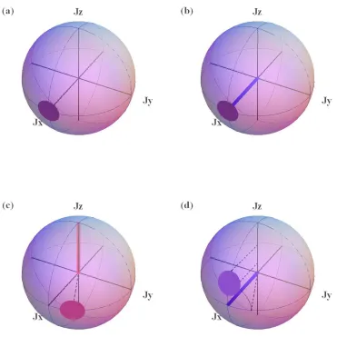
Figure 3.2: Representation of the interferometric sequence on the Bloch sphere: the
initial state (a) is represented by a disk centered around the mean value of the
momentum operators and with radius given by its spread. The first π/2 pulse (b) rotates the disk around its axis, it is followed by a phase accumulation (c) and the
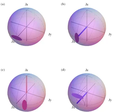
Figure 3.3: Representation of the interferometric sequence for a squeezed state on
the Bloch sphere: the initial state (a) is represented by an ellipse centered around
the mean value of the momentum operators and with axis given by its spreads.
desirable. The use of a system with tunable interactions is therefore necessary, on
the one hand, to exploit the interactions to create a squeezed state and, on the other,
to reduce the interactions to zero during the interferometric sequence, allowing for
long phase accumulation.
3.1.2
Entanglement and Fisher information
The resource exploited in order to beat the SQL in the example of the last section is
actually entanglement. The system cannot be described any longer as an ensemble
of independent particles but will be in an entangled state because of the introduction
of an interaction term in the Hamiltonian. However, not all entangled states are
actually able to lead to sub-shot noise sensitivity, but only a part of them[37].
Entanglement is a necessary condition but not sufficient. In order to distinguish
useful entanglement, the tools of estimation theory are exploited. The interesting
quantity we have to introduce is the Fisher information. Let us start by defining
a parameter φ we want to measure and the generator of the translations of that parameter Gb by
idψ
dφ =Gψ .b (3.16)
The measurement itself is performed by collapsing the wavefunction ψ onto the eigenstates of the measured quantity |ni. The probability to measure n, given the true value ofφ, is, therefore:
P(n|φ) =|hn|ψ(φ)i|2 . (3.17) Under this assumptions we can write the Fisher information F as:
F =
Z
P(n|φ)
dlog(P(n|φ))
dφ
2
dn . (3.18)
The relevance of the Fisher information is related to the Cramer-Rao lower bound
independent measurements to
∆φ = √1
mF . (3.19)
In the case of independent particles, it can be proven that the Fisher information is
additive
|ψi=⊗Ni=1|ψii (3.20)
F(|ψi) =
N
X
i=1
F(|ψii) . (3.21)
In connection to the uncertainty principle, an upper bound for the Fisher information
is given by:
F ≤4∆2G .b (3.22) By using these properties of the Fischer information, we can derive the SQL and the
ultimate limit to the sensitivity or Heisenberg limit (HL). If we deal with independent
particles, the Fisher will have the following upper bound:
F(|ψi) =
N
X
i=1
F(|ψii)≤N Fmax ≤N∆2maxG .b (3.23)
The maximum uncertainty of an operator can be realized by using an equal
super-position of its eigenstates with maximum and minimum eigenvalues
|ψi=⊗Ni=1|minii√+|maxii
2 . (3.24)
The value of ∆2
maxGb in the single particle case is going to be a constant. The
sensitivity limit therefore reads
∆φ∝ √1
mN (3.25)
which is the SQL. If instead we relax the independent particles assumption, we can
only rely on the upper limit for the Fisher information. Proceeding as before, we
time in a many-body Hilbert space. If the operator is a single particle one, the
maximum (minimum) eigenvalue is given by all particles being in the higher (lower)
single particle eigenstate. The superposition of this two states is called NooN-state
or, sometimes, a Schr¨odinger cat
|ψi= |min1, min2, ..., minNi√+|max1, max2, ..., maxNi
2 . (3.26)
The uncertainty ∆2
maxGb in this case is N2 times larger than in the single particle
case, leading to the HL
∆φ ∝ √1
mN . (3.27)
In principle a NooN-state can be experimentally realized by driving the system
into the ground state in presence of strong attractive interactions in a double well
|ψi= |N,0i√+|0, Ni
2 .
1 (3.28)
The BEC is anyway not stable in such a situation2. A more feasible strategy is to
use strong repulsive interactions to drive the system in a twin-Fock state
|ψi=
N 2, N 2 . (3.29)
Thia state is characterized by an exactly half filling of both wells. The uncertainty
for it is larger than the one given by the NooN state, nevertheless the scaling with
N of the uncertainty of the phase measurement can be proven to be the same. Such highly entangled states have anyway drawbacks, since they are more subject
to any form of loss or decoherence than the normal product states. As an example
we can imagine to have prepared a NooN state and, by some process (as three body
losses or collisions with the background gas), one atom is lost from the double well.
1here, differently from the previous analysis, the mean occupation of the wells (the value of
nl, nr) is indicated to describe the state instead of the single particle state.
2a more effective strategy to create a noon state that does not involve attractive interactions
It is in principle possible to get informations about the state of the system by using
a suitable detector to trace the lost atom back to its original position in one of the
two wells. The system therefore is forced to collapse in only that one well, losing its
Chapter 4
Experimental apparatus
In this chapter I describe the realized experimental apparatus, which comprises of a
great part of my PhD work. The design of the apparatus had to take into account the
crucial aspects of laser and evaporative cooling of potassium as well as the required
conditions to perform high-precision interferometry. The main components of the
apparatus are presented in Fig.4.1. The system is composed of three main vacuum
chambers. In the first one, the atoms are collected from the background gas into
a two-dimensional magneto-optical (2D-MOT) trap, producing an atomic beam.
The atomic beam is directed to the second chamber where a three-dimensional
magneto-optical trap (3D-MOT) is hosted. In the 3D-MOT, the sample is cooled
to sub-Doppler temperatures. Once the atoms are prepared, they get transferred to
a magnetic trap. Such magnetic trap is moved by mean of a motorized translation
stage up to the third chamber (science chamber). In the science chamber the atoms
gets trapped into a dipole trap and evaporative cooling performed employing a
Pump1
Pump2
Pump3
2D-MOT
3D-MOT
Magnetic transport
Science chamber
Rear window
Figure 4.1: Simplified sketch of the main parts of the apparatus. The atoms from
the 2D-MOT are collected into the 3D-MOT. Moving colis are used to transfer the
atoms from the 3D-MOT chamber to the science chamber. The last vacuum pipe is
not parallel to the magnetic coil motion, for this reason the last part of the atomic
transfer has to be purely magnetic from the moving coils to the Feshbach coils. The
distance between the coil’s centers is about 10 cm. This allows for an extra optical
access through the rear window.
4.1
Experimental design
A very long lifetime of the atomic sample is desired for high resolution interferometry,
in order to achieve long phase accumulation. A very large optical access is also
necessary, because of the particular implementation of a light-made double-well
interferometer and of all-optical evaporation of the atomic sample. A large optical
access will enable us to use many trapping beams as well as to implement high
spatial resolution imaging.
In order to satisfy these conditions, we decided to use a scheme with three
vacuum chambers (see Fig.4.2). In the passage from each chamber to the next one,
a differential pumping stage reduces the pressure an thus it increases the lifetime of
Figure 4.2: Overview of the vacuum system. The three chambers are indicated
as 2D-MOT, 3D-MOT and science chamber. The position of the potassium solid
sample and of the potassium dispensers is indicated. To make the sublimation pump
visible, the vacuum pipe containing it was omitted from the drawing.
pressure of potassium vapor, of around 10−8 mbar, ensures a fast loading rate and
thus a large atomic flux towards the second cell. In the second cell, large laser beams
are used in order to trap a large number of atoms; here the pressure drops to around
10−9 mbar. The atoms are then transferred to the last chamber, using trapping coils
mounted on a moving cart. The last chamber allows a very large optical access, due
to its shape and to the absence of MOT beams for the cooling. The last differential
pumping stage also allows to achieve pressures as low as 10−11 mbar.
4.2
Choice of the building materials
Since the interferometer will be performed with magnetic atoms, particular care was
taken in order to reduce any magnetic field fluctuation or instability, in particular
table, that holds the vacuum system, is a custom TMC realization made of the 304
low magnetic stainless steel alloy. The 316L alloy, characterized by an even lower
magneticity, is used for the topmost and lowermost planes of the table.
The MOT chambers are realized in Ti-6Al-4V, for its low magneticity (four
times lower than for steel) and high resistivity. High resistance materials allows for
fast variation of the magnetic fields thanks to the rapid fall off of Eddie currents.
Components that are close to the atoms, like vacuum chambers, pipes, valves and
bellows through which the sample is passing during the transport, are realized in
low magneticity stainless steel compounds like the SS304 or the SS316 compounds.
For the vacuum connections towards the pumps the SS321 alloy is employed instead.
The science cell itself is realized in glass and it is placed with its center 15cm away
from the first metallic element (its own vacuum valve), realized in 316L stainless
steel. The Feshbach coils, used to tune the interactions, are held by a fully plastic
mount and kept in physical contact with the cooling water.
4.3
Vacuum pumps
In this section, I will justify the choices made for what concerns the pumping of
the vacuum assembly and I will give indications of the achieved vacuum levels in
the apparatus with their limitations. Finally, I will be report the measurements
of the achieved atomic sample lifetime in the various vacuum sections, yielding
the final confirmation of the achievement of low pressures. The sample lifetime is
proportional to the inverse of the background pressure. A simple calculation based
on the background collisions cross section yields a lifetime of the sample between
2 and 8 s (depending on the chemical composition of the background gas) for a
pressure of 10−9 mbar.
that eliminates condensed water laying onto the internal surfaces of the system and
most of the hydrogen accumulated in the steel during its fusion process. We baked
all the steel components separately in an oven for approximately one day at 400◦ C
to eliminate most of the hydrogen. After the system was assembled we baked the
2D-MOT and 3D-MOT parts at 120◦ C for five days. The chosen temperature was
limited by the sealing glue used for the vacuum windows. The science chamber
section was added later on and separately baked. Since there was no glue on this
section, the baking temperature was chosen to be 200◦ C; again the procedure lasted
for five days.
In Fig.4.2, the position of the various pumps is depicted. The pumps used in the
first two cells are Varian Diode Vaclon ionic pumps with different pumping speeds.
These pumps are particularly indicated for pumping of active gases such as N2, O2,
CO2, H2. Especially Hydrogen is supposed to be abundantly outgassed from the steel
composing the vacuum chambers due to its fabrication process. For the pumping of
the science chamber we chose, instead, a StarCell ion pump in combination with a
Titanium sublimation pump (TSP). The StarCell achieves slightly lower pumping
speeds for active gases than the Diode model but can pump much better noble gases
as He and Ar or Methane. The pumping of active gases is provided by the Titanium
sublimation pump in this case.
The current reading on the pumps provides an indication of the pressure in
the first two vacuum chambers. The reading performed this way is limited by
leakage currents of about 10 µA. This represents a limit pressure reading of about 10−7-10−8 mbar. Both the pumps reports current readings comparable to their
leakage currents. Close to the StarCell a Varian UHV-24p nude Bayard-Alpert type
ionization gauge tube was placed. Its pressure reading is 7×10⁻¹² mbar which is
represents the lower detectable value. However, those readings are performed close
conductances and the outgassing rates.
The 2D-MOT section of the vacuum is pumped by a 20 l/s Varian Diode Vaclon
ion pump. The effective pumping speed at the chamber decreases to 6.8 l/s due
to the conductance of the connections (all the values are calculated for air). By
calculating the outgassing of the various surfaces, we estimate an achievable
pres-sure of 1.5×10⁻⁹ mbar. The conductance to the 3D-MOT chamber is negligible
(0.03 l/s). During normal operation, the outgassing rate is deliberately increased by
releasing potassium in the chamber, either by passing current through dispensers or
by heating a solid sample. We measured the absorption of a laser beam tuned to
the D2 resonance to estimate the partial pressure of potassium in the chamber. We
estimated a partial pressure of 10−8 mbar, under the assumption that the atomic
velocity distribution is in thermal equilibrium at room temperature.
For the 3D-MOT we used a 55 l/s Varian Diode Vaclon ion pump. The effective
pumping speed at the chamber is estimated to be 17 l/s. The leading contribution
to the outgassing comes from the sealing glue used for the windows. The nominal
value for the outgasing of such a glue is 1.3×10⁻⁹mbar×l/(s×cm2). Such outgassing
rate would limit the attainable press