On Optimizing Distributed Tucker Decomposition for Dense Tensors
Venkatesan T. Chakaravarthy, Jee W. Choi, Douglas J. Joseph, Xing Liu, Prakash Murali, Yogish Sabharwal, Dheeraj Sreedhar
IBM Research
{vechakra,prakmura,ysabharwal,dhsreedh}@in.ibm.com {jwchoi,djoseph,xliu}@us.ibm.com
Abstract—The Tucker decomposition expresses a given ten-sor as the product of a small core tenten-sor and a set of factor matrices. Our objective is to develop an efficient distributed implementation for the case of dense tensors. The implementa-tion is based on the HOOI (Higher Order Orthogonal Iterator) procedure, wherein the tensor-times-matrix product forms the core routine. Prior work have proposed heuristics for reducing the computational load and communication volume incurred by the routine. We study the two metrics in a formal and systematic manner, and design strategies that are optimal under the two fundamental metrics. Our experimental evaluation on a large benchmark of tensors shows that the optimal strategies provide significant reduction in load and volume compared to prior heuristics, and provide up to 7x speed-up in the overall running time.
Keywords-Tensor compression, HOSVD, HOOI.
I. INTRODUCTION
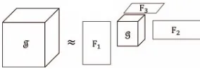
Tensors are the higher dimensional analogues of matrices. While matrices represent two-dimensional data, tensors are useful in representing data in three or higher dimensions. Tensors have been studied extensively via generalizing con-cepts pertaining to matrices. The Tucker decomposition [1] is a prominent construction that extends the singular value decomposition (SVD) to the setting of tensors. Given an N-dimensional tensor T, the decomposition approximately expresses the tensor as the product of a smallN-dimensional core tensorGand a set ofNfactor matrices, one along each dimension (or mode); see Figure 1 for an illustration. The core is much smaller than the original tensor leading to data compression. Prior work [2] has reported compression rates to the tune of 5000 on large real tensors. Apart from data compression, the decomposition is also useful in analysis such as PCA, and finds applications in diverse domains such as computer vision [3] and signal processing [4]. A detailed discussion on the topic can be found in the excellent survey, by Kolda and Bader [5].
Tucker decomposition has been well-studied in sequential, shared memory and distributed settings for both dense and sparse tensors (e.g., [2], [6], [7]). Our objective is to develop an optimized implementation for dense tensors on dis-tributed memory systems. The implementation is based on the popular STHOSVD/HOOI procedures. The STHOSVD (Sequentially Truncated Higher Order SVD) [8] is used to produce an initial decomposition. The HOOI (Higher Order Orthogonal Iterator) [9] procedure transforms any
Figure 1: Illustration for Tucker decomposition on a 3-dimensional tensor: T - input tensor, G - core tensor, Fn - factor matrices.
given decomposition to a new decomposition with the same core size, but with reduced error. The procedure is applied iteratively so as to reduce the error monotonically across the iterations. We focus on the latter HOOI procedure which is invoked multiple times. The tensor-times-matrix product (TTM) component forms the core module of the procedure. Prior work has proposed heuristic schemes for reducing the computational load and communication volume of the component. Our objective is to enhance the performance by constructing schemes which are optimal in these two fundamental metrics.
Prior Work
Heuristics for computational load: The TTM compo-nent comprises of a set of tensor-times-matrix multiplication operations. Based on the observation that the operations can be rearranged and reused in multiple ways, prior work has proposed heuristics for reducing the computational load. A naive scheme for implementing the component performs N(N −1) TTM operations. Baskaran et al. [10] focused on reducing the number of TTM operations, and proposed a scheme with (approximately) N2/2 operations, which was further improved to NlogN by Kaya and Uc¸ar [11]. However, minimizing the number of TTM operations is not sufficient and it is crucial to consider the cost of the operations, especially in the context of dense tensors. Austin et al. [2] measure the cost in terms of the number of floating point operations (FLOP). They empirically showed that the performance of the navie scheme can be improved by permuting (ordering) the modes of the input tensor and proposed a greedy heuristic for mode ordering. A similar heuristic is given by Vannieuwenhoven et al. [8].
parallel distribution which generalizes the block distribution technique used in the context of matrices. The processors are arranged in the form of an N-dimensional grid and a tensor is partitioned into blocks by imposing the grid on the tensor; the blocks are then assigned to the processors. They showed that the communication volume is determined by the choice of the grid, and presented an empirical evaluation of the effect of the grid on the communication volume.
Our Contributions
Our objective is to enhance the performance of distributed Tucker decomposition for dense tensors by designing opti-mal schemes for the two metrics and we make the following contributions.
• Optimal TTM-trees:As observed in prior work [11], the different TTM schemes can be conveniently represented in the form of trees, called TTM-trees. We present an efficient algorithm for constructing the optimal TTM-tree, the one having the least computational load, mea-sured in terms of number of floating operations (FLOP).
• Dynamic Gridding: Prior work uses a static gridding scheme, wherein the same grid is used for distributing the tensors arising in the different TTM operations. We propose the concept ofdynamic griddingthat uses dif-ferent grids tailored for the difdif-ferent operations, leading to significant reduction in communication volume, even when compared to the optimal static grids.
• Optimal Dynamic Gridding: We present an efficient algorithm for finding the dynamic gridding scheme achieving the optimal communication volume. Our distributed implementation builds on the work of Austin et al. [2] and incorporates the optimal schemes described above. We setup a large benchmark consisting of about1700 tensors whose metadata are derived from real-life tensors. Furthermore, we also include a set of tensors with metadata derived from simulations in combustion science. Our exper-imental evaluation on the above benchmark demonstrates that the combination of optimal trees and the dynamic gridding scheme offers significant reduction in computa-tional load and communication volume, resulting in up to 7-factor improvement in overall execution time, compared to prior heuristics. To the best of our knowledge, our study is the first to consider optimal algorithms for the Tucker decomposition.
We note that prior work [8], [2] has provided evidence that STHOSVD may be sufficient for particular application domains. They present experimental evaluations on a sample of tensors arising in image processing and combustion sci-ence showing that for these tensors, STHOSVD is sufficient and HOOI does not provide significant error reduction. Our optimizations on HOOI would be useful for other tensors/domains where HOOI provides error reduction over STHOSVD. Furthermore, the ideas developed in this paper can be recast and used for improving STHOSVD as well.
Related Work
Tucker decomposition has been studied in sequential and parallel settings for dense and sparse tensors. For dense tensors, the MATLAB Tensor Toolbox provides a sequential implementation [12]. Li et al. [13] proposed performance enhancements for a single TTM operation and their tech-niques can be incorporated within our framework. Austin et al. [2] described the first implementation for distributed memory systems, wherein they proposed heuristics for mode ordering and experimentally demonstrated the effect of grid selection on communication time. For sparse tensors, se-quential [7], shared memory [10] and distributed implemen-tations [6] are known. Other tensor decompositions have also been considered (see [5]). In particular, CP decomposition which generalizes the concept of rank factorization has been well studied (e.g. [14]).
Note: Certain details are omitted from the discussion in this paper, due to space limitations. These can be found in the full version of the paper (available as ArXiv preprint).
II. TUCKERDECOMPOSITION
A. Preliminaries
Fibers: Consider an N-dimensional tensor T of size
L1×L2× · · · ×LN. Let|T|denote the cardinality (number of elements) of the tensor. The elements of T can be canonically indexed by a coordinate vector of the form l1, l2, . . . , lN, where each indexln belongs to [1, Ln], for all modes 1 ≤ n ≤ N. A mode-n fiber −→x is a vector of length Ln, containing all the elements that differ on the
nth coordinate, but agree on all the other coordinates, i.e., l1, . . . , ln−1,∗, ln+1, . . . lN. The number of mode-nfibers is|T|/Ln. In the analogous case of matrices, two types of fibers can be found: row vectors and column vectors.
Tensor Unfolding: The tensor T is stored as a matrix and there areN different matrix layouts are possible, called the unfoldings. The mode-n unfolding of T refers to the matrix whose columns are the mode-nfibers of the tensor. The columns are arranged in a lexicographic order (the details are not crucial for our discussion). This matrix is of sizeLn×(|T|/Ln), and we denote it asT(n).
TTM-Chain: The TTM-chainoperation refers to mul-tiplying T along multiple distinct modes. For two modes
n1 and n2 and matrices A1 and A2, we first multiply T by A1 along mode n1, and then multiply the output tensor along mode n2 by A2. An important property of the operation is commutativity [9], namely the two TTM operations can be performed in any order: (T×n1A1)×n2 A2= (T×n2A2)×n1A1. In general, for a subset of distinct modesS={n1, n2, . . . , nr}, and matricesA1,A2, . . . ,Ar, where Aj has size Kj × Lnj, the output is a tensor
Z=T×n1A1× · · · ×nrAnr. The length ofZremains the
same as T along modes not belonging to S, and changes to Kj, for all nj ∈ S. Commutativity implies that the multiplications can be performed in any order.
B. Tucker Decomposition and HOOI
The Tucker decomposition ofT approximates the tensor as the product of a core tensorG of sizeK1×K2× · · · × KN, with each Kn ≤ Ln, and a set of factor matrices F1,F2, . . . ,FN: T ≈ Z= G×1F1×2F2× · · · ×N FN. The factor matrixFn has sizeLn×Kn. The decomposition compresses the length of T along each mode from Ln to Kn. We write the decomposition as {G;F1,F2, . . . ,FN}. The error of the decomposition is measured by comparing the recovered tensor Z and the input tensor T under the normalized root mean square metric.
The HOOI procedure [9] transforms a given decomposi-tion into a new decomposidecomposi-tion having the same core size, but with reduced the error. Given an initial decomposition, the procedure can be invoked repeatedly to reduce the error monotonically, until a desired convergence is achieved. An initial decomposition can be found using methods such as STHOSVD [8].
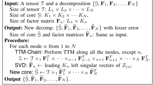
The HOOI procedure (a single invocation), shown in Figure 2, takes as input the tensor T, and a decomposition {G,F1,F2, . . . ,FN} with core sizeK1×K2× · · · ×KN. It produces a new decomposition{G˜,F1,F2, . . . ,FN}with lesser error, but having the same core and factor matrix sizes. For computing each new factor matrix Fn, the procedure utilizes the alternating least squares paradigm and works in two steps. First, it performs a TTM-chain operation by skipping mode n and multiplying T by the transposes of all the other factor matrices Fj (with j = n) and obtains a tensor Z. The tensor Z has length compressed from Lj to Kj along all modes j=n. In the next step, it performs an SVD on Z(n), the mode-nunfolding of the Z. The new factor matrix Fn is obtained by arranging the leading Kn singular vectors as columns. Once all the new factor matrices are computed, the new core tensor is computed.
Figure 3 (a) depicts the process in the form of a tree. The root represents the input tensorT, each node with label
n represents multiplication along mode n, and each leaf represents a new factor matrix. For dense tensors, the SVD operations tend to be inexpensive (see [2]). Therefore, we
Input:A tensorTand a decomposition{G,F1,F2, . . . ,FN} Size of tensorT:L1×L2× · · · ×LN
Size of coreG:K1×K2× · · ·KN, Size of factor matrixFn:Ln×Kn
Output:New decomp.{G˜,F1,F2, . . . ,FN }with lesser error Size of coreG˜and factor matricesFn : Same as input. Procedure:
For each modenfrom1toN
TTM-Chain:Perform TTM along all the modes, exceptn.
Z←T×1FT1 × · · · ×n−1FTn−1×n+1FTn+1× · · · ×NFTN. SVD:Fn ←leadingKnleft singular vectors ofZ(n) New core:˜G←T×1FT1 × · · · ×NFTN
Output{G˜,F1,F2, . . . ,FN }.
Figure 2: HOOI Procedure
focus on optimizing the TTM component comprising of the
NTTM-chains, from the perspectives of computational load and communication volume.
III. COMPUTATIONALLOAD
The TTM component performs N TTM-chains, each involving (N−1) TTM operations. Commutativity allows us to rearrange and reuse the operations in multiple ways, all of which can be represented in the form of TTM-trees, as observed in prior wok [11]. We measure the computational load of a tree by the number of floating point operations incurred. Our objective is to design an efficient algorithm for finding the optimal TTM-trees. Below, we first formalize the above model and rephrase prior schemes, and then describe the optimal algorithm.
A. TTM-trees and Cost
In a TTM-tree, the root represents the input tensor T, each leaf node represents a unique new factor matrix and each internal node (nodes other than the root and the leaves) represents TTM along a particular mode. The root-to-leaf path leading to a new factor matrix Fn realizes the TTM-chain required for computingFn.
1) TTM-Trees: Formally, aTTM-treeH is a rooted tree with a functionlbl(·)that assigns a labellbl(u)to each node
usuch that the following properties are satisfied: (i) the label of the root node is lbl(root) = T; (ii) there are exactly N
leaves, with each leaf u being labeled with a unique new factor matrix lbl(u) = Fn; (iii) each internal node u is labeled with a mode lbl(u) ∈ [1, N]; (iv) for each leaf u
with label lbl(u) = Fn, the path from the root to u has exactly(N−1)internal nodes and all the modes except n
appear on the path.
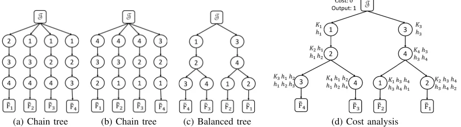
(a) Chain tree (b) Chain tree (c) Balanced tree (d) Cost analysis
Figure 3: Example TTM-trees and cost analysis. Tree (a) and (b) are both chain trees, but use different orderings,1,2,3,4 and 4,3,2,1, respectively.
Given a treeH, the HOOI procedure can be executed via a natural top-down process by associating each node with an input tensorIn(u)and an output tensorOut(u). For the root node, In(root) = Out(root) = T. Each internal node u with lbl(u) = n takes as input the tensor output by its parentv, multiplies it along modenby the factor matrixFTn, and outputs the resultant tensor, i.e., In(u) =Out(v)and Out(u) =In(u)×nFTn. Each leaf nodeuwithlbl(u) =Fn constructs the new factor matrixFnby performing an SVD on the tensor output by its parent. The correctness of the procedure follows from the commutativity property of the TTM-chain operation. In the above procedure, we reuse the tensor output by a node for processing all its children. By executing the process via an in-order traversal, we can ensure that the maximum number of intermediate tensors stored at any point is bounded by the depth of the tree.
2) Computational Load: We define the cost (or com-putational load) of a TTM-tree H to be the number of floating point operations (FLOP) performed. Each internal node u with labellbl(u) =n executes the TTMOut(u) = In(u)×nFTn. Recall that the operation involves the matrix-matrix multiplication, wherein the matrix-matrix FTn is multiplied by the mode-n unfolding of In(u). The matrix has size Kn×Lnand the unfolded tensor has sizeLn×(|In(u)|/Ln) and so, the cost of the TTM isKn· |In(u)|. The cardinality of the output tensor is|Out(u)|= (Kn/Ln)|In(u)|; namely, the node compresses the tensor by a factor(Kn/Ln). We can compute the cost incurred at all the nodes and the cardinality of their output tensors by performing the above calculations in a top-down manner. Then, the cost of the treeH is given by the sum of costs of its internal nodes. We can see that each modenis associated with two parameters: acost factor Kn and acompression factor (Kn/Ln), which we denote as hn. At each node, the cost incurred and the cardinality of the output tensor can be expressed in terms of these two parameters.
Figure 3 (d) provides an illustration. The cost incurred and the cardinality of the output tensor are shown at each
node. For the ease of exposition, we have normalized all the quantities by|T|. The root node has cost0and its cardinality of its output is|T|, which is1after normalization. Each node u with labelnincurs a cost ofKn times the cardinality of the tensor output by its parent; it outputs a tensor having cardinality compressed by a factor hn.
B. Prior Schemes
We rephrase the prior schemes in terms of TTM-trees. Chain trees: These trees encode the naive scheme, with N independent chains, each comprising of (N−1) nodes (see figure 3 (a) and (b)).
Balanced trees: Chain trees performN(N−1)TTMs. Kaya and Uc¸ar [11] improved the count to approximately NlogN, via a divide-and-conquer strategy. The idea is to divide the modes into two groups{1,2, . . . , m} and{m+ 1, m+ 2, . . . , N}, wherem=N/2. We create a chain of nodes of lengthmwith labels from the first group and attach it to the root. Then, we recursively construct a subtree for the second group and attach it at the bottom of the chain. We then repeat the process by reversing the roles of the two groups. Figure 3 (c) shows an example for N = 4. The number of internal nodes is approximatelyNlogN.
C. Constructing Optimal Trees
In this section, we present our algorithm for constructing the optimal TTM-tree, the tree with the minimum cost. The algorithm is based on dynamic programming and runs in timeO(4N). In practice, the algorithm takes negligible time, since the number of dimensions of dense tensors is fairly small (typically,N≤10).
Towards developing the dynamic programming algorithm, we first claim that the optimal TTM-tree is binary, namely every node has at most two children. The proof is based on the observation that if a node u has three children, then the children can be rearranged so that only two of the nodes remain as children of u. The proof can be found in full version of the paper. Below, we identify a set of subproblems and derive a recurrence relation relating them. This is followed by a description of the algorithm and an analysis of the running time.
1) Subproblems: Consider any binary treeH and letube an internal node in it. With respect tou, the modesncan be partitioned into three groups: (i) pre-multiplied: nis found along the path from the root tou, includingu; (ii)computed underu: the leaf bearing labelFnis found under the sub-tree rooted at u; (iii) ndoes not belong to either category. Let
P,QandRdenote the set of modes belonging to the three categories. For an illustration, consider the tree in Figure 3 (c) and let u denote the right child of the root labeled 3; with respect this node, P = {3}, Q= {1,2} and R =
{4}. Notice that the triple(P, Q, R)forms a partitioning of [1, N]. We can characterize any node u in a TTM-tree via the above3-partition.
We next make an observation regarding the setR. Con-sider the stage in the HOOI execution, wherein we have completed the processing of the node u. At this stage, we have already completed multiplication along all modes in
P. For any mode n ∈ Q, the corresponding TTM-chain involves multiplication along all modes, exceptn. Of these modes, we are yet to perform multiplication along the modes inRandQ\{n}. The multiplications along modes inRare common to the TTM-chains corresponding to all the modes inQ. Therefore, at this stage, we can potentially select any mode from R, perform multiplication along the mode and reuse the output tensor. Hence, we call the modes in R as reusable. For instance, mode 4 is reusable in the example discussed earlier (Figure 3).
The idea behind the dynamic programming algorithm is to consider a subproblem for each possible triple(P, Q, R)as follows: construct the optimal subtree given that the modes inP have been multiplied already, the modes inQneeds to be computed and R are the reusable modes. We formalize the concept using the notion of partial TTM-trees.
Partial TTM-tree: Consider a triple (P, Q, R) with |Q| ≥1. LetT[P]denote the tensor obtained by multiplying Tby the factor matrices along all the modes found inP. A partial TTM-tree for (P, Q, R) is a rooted tree with labels
on its nodes such that the following properties are satisfied: (i) the root is labeled X=T[P]; (ii) there are exactly |Q|
leaves, with each leaf ubeing labeled with a unique factor matrixFn, forn∈Q; (iii) each internal nodeu is labeled with a mode from[1, N]\P; (iv) for each leaf nodeuwith labelFn, the path from the root touhas exactlyN−|P|−1 internal nodes and all the modes exceptP∪ {n}appear on them. Figure 4 shows two example partial-TTM trees for the tripleP ={3},Q={1,2} andR={4} discussed earlier. The cost of a partial-TTM tree is defined analogous to the usual TTM-trees. LetH∗(P, Q, R)denote the optimal par-tial TTM-tree for the triple(P, Q, R)and letcost∗(P, Q, R)
be the cost of the optimal tree. The optimal tree for the original problem is given by H∗(P, Q, R) with P = ∅, Q= [1, N]and R=∅.
2) Recurrence Relation: We discuss the subproblem structure and derive a recurrence relation. Consider a triple (P, Q, R). Since optimal trees are binary, the root of
H∗(P, Q, R) can have either one or two children. The recurrence relation considers both the possibilities, which we refer to asreuseandsplitting.
Reuse: This option is available, if R =∅. In this case,
we select a mode n ∈ R and multiply X = T[P] along mode n. The result is then reused for computing the new factor matrices of all the modes in Q. In terms of TTM-trees, the operation corresponds to adding a single child with labelnto the root of the partial TTM-tree. Once the above TTM operation is performed, we are left with solving the subproblem corresponding to the triple(P∪{n}, Q, R\{n}). The cost is given by sum of the cost of the TTM operation X×nFTn and the cost of recursively solving the subproblem. Recall that the former cost is Kn· |X|. The latter cost is cost∗(P∪{n}, Q, R\{n}). In the above process, any mode from R can be reused and we can find the best option by considering all the choices.
Splitting: The second possibility is to split (or partition)
Qinto setsQ1 andQ2 and independently solve the triples
(P, Q1, R) and (P, Q2, R). The total cost is given by the sum of costs of optimal subtrees of the two subproblems, i.e., cost∗(P, Q1, R) +cost∗(P, Q2, R). Any (non-trivial) partition (Q1, Q2) of Q with Q1, Q2 = ∅ can be used in the above process and the best choice can be found by an exhaustive search.
The above discussion yields the following recurrence relation for computing the optimal cost of a triple(P, Q, R):
cost∗(P, Q, R) = min{cost∗reuse,cost∗split},where
cost∗reuse = min
n∈RKn· |T[P]|+cost
∗(P∪ {n}, Q, R\ {n})
cost∗split = min Q1,Q2⊆Q
cost∗(P, Q1, R) +cost∗(P, Q2, R).
Figure 4: Example partial TTM-trees withN = 4,P ={3}, Q={1,2}, andR={4}.X=T[P] =T×3FT3
number of table lookups is at most2·4N. Thus, algorithm runs in time O(4N).
Remarks: Given that N is small, we may consider constructing the optimal TTM-trees via an exhaustive search. A naive search over all TTM-trees is prohibitively expensive. The TTM operation corresponding to a mode n involves multiplication along all the other(N−1)modes, which can be performed in any of the ((N−1)!) orderings. Over all the nodes, the number of combinations is((N−1)!)N), all which can be realized as chain trees. We can expedite the search by considering only the binary TTM-trees. We are not aware of any closed form expression for the number of binary TTM-trees. We note that our algorithm can be mod-ified to enumerate all these trees. Instead of enumeration, the algorithm incorporates memoization and computes the optimal tree efficiently in timeO(4N).
IV. COMMUNICATIONVOLUME
Our strategy is to fix a TTM-treeH(based on the heuristic or the optimal tree) and devise schemes for minimizing the volume. Our distributed implementation uses the same strategy as that of Austin et al. [2] for distributing the tensors and performing TTM in a distributed manner. We propose a dynamic gridding scheme that offers significant reduction in volume and design an efficient algorithm for finding the optimal scheme.
A. Distributed Setup
Tensor Distribution: Fix a TTM-treeHand letP be the number of processors. We arrange the processors in anN -dimensional gridg=q1×q2×· · ·×qN such thatP =jqj. To distribute a tensor, we impose the grid on the tensor and partition it into P blocks, and assign each block to a processor; see Figure 5 (a) for an illustration. The input tensor T and all the intermediate tensors gets partitioned using the same grid.
Distributed TTM and Volume: Each nodeuwith label n and parent v performs the TTM operation Out(u) = In(u)×nFTn. For the gridg, we denote the communication volume incurred by the operation as vol(u, g). As observed in the prior work vol(u, g) = (qn −1)|Out(u)|; a brief outline of the argument in the following paragraph. The total communication volume of g, denoted vol(H, g), is defined to be the sum of volumes incurred at all the internal nodes.
Recall that the TTM operation Out(u) =In(u)×nFTn can be viewed as applying the linear transformation FTn to every mode-n fiber −→x of In(u). That is, we need to perform the matrix-vector product−→y =FTn · −→x. Since the factor matrices are small in size, we can afford to keep a copy of them at every processor. However, each mode-n fiber−→x gets distributed equally among someqn processors and so, computing the product requires a reduce operation. Similarly, the output fiber −→y must be distributed among the same processors using a scatter operation. See Figure 5 (b) for an illustration. The reduce-scatter operation is performed over the output fiber −→y of Kn, for which we incur(qn−1)Kn units of communication. Summed up over all the fibers, the total communication volume for the TTM is(qn−1)|Out(u)|.
In the above distribution method, if qn > Ln for some mode n, then some processor would receive an empty block while partitioning T. Similarly, if qn > Kn then same scenario would arise on some intermediate tensor. We avoid the load imbalance by considering only grids with qn ≤ Kn, for all n; we call these valid grids. In the rest of the discussion, unless explicitly mentioned, we shall only consider valid grids.
B. Finding the Optimal Static Grid
We observe that the optimal static grid, the one achieving the minimum communication volume, can be found via an exhaustive search in negligible time. The number of grids, including the invalid ones, is the same as number of ways in which the integer P can be expressed as the product of N factors, which we denoteψ(P, N). If the prime factorization ofP isP =pe1
1 ·pe22· · ·pess, then we have that ψ(P, N) =
s
i=1
ei+N−1 N−1
When the quantity becomes large, the search can be paral-lelized in a straightforward manner. Even for the extreme case of P = 220 and N = 10, the number of grids to be scanned per processor is approximately10.
C. Dynamic Gridding Scheme
(a) Example grids (b) Matrix-fiber multiplication
Figure 5: Distributed setup: (a) the two figures use the grids 4,2,1and2,2,2, respectively.
if the tensor output by the parentvis represented in a gridg and we have selected a different gridgfor representing it at u, then the tensor must be regridded (redistributed) among the processors. The process incurs a volume of |In(u)|. Thus, a dynamic grid scheme must decide whether or not to regrid at each node, and furthermore, if it decides to regrid, the new grid must be selected in a manner beneficial for the TTM operations performed later in the subtree, so that the overall communication is minimized.
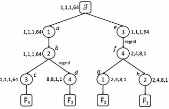
In Figure 6, we have shown an example, carefully con-structed so as to highlight the different aspects of dynamic gridding. Assume that the number of processors is P = 64 and the core is of size 8× 8× 8× 64. The choice of the initial grid 1,1,1,64 makes the TTM operations at nodes a, b, c and e are communication-free. However, the grid is not suitable for the TTM at noded, since the volume incurred is63× |Out(d)|. Instead, we switch to a new grid 8,8,1,1, making the operation communication-free. We perform another regrid operation at node f by selecting the new grid2,4,8,1, The choice of the new grid is motivated by the following considerations. The subtree beneathf does not involve any TTM along mode 3and so, it is prudent to assign a high value along the mode. However, we must select a valid grid, and the constraint implies that the maximum possible value is 8 (since the core length along mode 3 is K3 = 8). We next assign a value of 1 to mode 4, thereby making the TTM at nodedcommunication-free. The remaining of value of8is assigned to the modes1and2in a balanced manner.
Dynamic Grid Scheme: Formally, a dynamic grid scheme is a mapping π that associates a grid π(u) with each nodeu. The volume incurred by the scheme, denoted dvol(H, π)is defined as follows. For each nodeuwith label nand parentv, we compute the volume incurred at the node as the sum of two components: (i) TTM operation volume: (qn−1)|Out(u)|, where qn is the assignment to mode n underπ(u); (ii) regridding volume: ifπ(u)is the same as the parent grid π(v), then the volume is zero, and otherwise, it is|In(u)|. The volume of the schemeπ, denoteddvol(H, π), is defined to be the sum of communication incurred over all the nodesu. At the root node, we represent the input tensor T under the grid π(root) and we do not have the regrid
Figure 6: Example dynamic grid scheme
option. Let dvol∗(H) denote the optimal communication volume achievable among all dynamic grid schemes, and letOpt(H)denote an optimal scheme.
D. Optimal Dynamic Gridding Scheme
In this section, we develop an efficient dynamic program-ming algorithm for computing the optimal dynamic grid scheme for a given tree H. For a nodeu, letH(u)denote the subtree rooted at u. A partial grid scheme for H(u) refers to a mappingπ that specifies a grid for each node in H(u). For each node uand each grid gpar, we shall define
a subproblem with the following connotation: assuming that the tensor output by the parent is represented under the grid gpar, find the optimal partial grid scheme for the subtree H(u). We solve these subproblems via a bottom-up traversal of the tree, wherein the optimal solution at u is computed from the optimal solutions of its children.
1) Subproblems: Consider a pair (u, gpar), whereu is a
node andgpar is a grid. For a partial grid schemeπ for the
subtree, let dvol(H(u), π|gpar) denote the volume incurred
otherwise, it is |In(z)|. Then, the volumedvol(Hu, π|gpar)
is defined to be the sum of volumes associated with all the nodesz∈H(u). Letdvol∗(H(u)|gpar)denote the minimum
volume possible among all partial grid schemes π. We do not regrid at root and so, define dvol∗(H|gpar) to be the
minimum volume given thatT is represented undergpar.
2) Recurrence Relation: We derive a recurrence relation for computing dvol∗(H(u)|gpar). Let v1, v2, . . . , vs be the children of u. In determining the optimal partial scheme, we have two options: (i) regrid: select a new grid rg∗(u)
for representing In(u); (ii) do no regrid: represent In(u)
under the given gridgpar. In the first case, we selectrg∗(u)
to be the grid yielding the minimum volume for the child subtrees:
rg∗(u) = argming s
j=1
dvol∗(H(vj)|g).
We can now write the recurrence for dvol∗(H(u)|gpar). Letnbe the label ofuandvbe the parent ofu. Letgpar=
p1, p2, . . . , pNand letrg∗(u) =q1, q2, . . . , qN. Then:
dvol∗(H(u)|gpar) = min{vol∗1,vol∗2},where
vol∗1=|In(u)|+(qn−1)|Out(u)|+ s
j=1
dvol∗(H(vj)|rg∗(u))
vol∗2= (pn−1)|Out(u)|+ s
j=1
dvol∗(H(vj)|gpar)
The two quantities correspond to the optimal solutions for the two choices of regridding and not regridding. In both the cases, we incur communication for the TTM operation and communication in the subtrees. In addition, the first case incurs a regrid volume of|In(u)|. Under the two choices, the
tensors In(u) and Out(u) get represented under the grids rg∗(u) and gpar, respectively. Consequently, the recursive
calls for the two choices are made with the corresponding grids. At the root node, we represent T under gpar and do
not regrid and so, we consider only the first choice at the root. The optimal volume for the whole tree dvol∗(H) is given by minimum ofdvol∗(H|gpar), over all the choices of
gpar and can be computed via enumerating the choices.
The algorithm can be implemented with a running time
O(|H| ·ψ(P, N)). As in Section IV-B, it can be parallelized so that the execution time is negligible in practice.
V. EXPERIMENTALEVALUATION
A. Distributed Implementation
The distributed implementation consists of two modules, aplanner that constructs TTM-trees and selects grids, and an engine, which implements distributed TTM, SVD and regrid (tensor redistribution in the case of dynamic gridding scheme) operations. The TTM operation is implemented
Tensor Dimensions Core Tensor Dimensions HCCI (672, 672, 627, 16) (279, 279, 153, 14) TJLR (460, 700, 360, 16, 4) (306, 232, 239, 16, 4) SP (500, 500, 500, 11, 10) (81, 129, 127, 7, 6)
Table I: Real tensors used in our study
using the algorithm proposed by Austin et al. [2]. We im-plement the SVD component using distributed Gram matrix computation (AAT) followed by eigen value decomposition (EVD) via dsyrk and dsyevx calls. All the processors use the same TTM-tree and there is synchronization at each tree node.
B. Setup
1) System: The experiments were conducted on an IBM BG/Q system. Each BG/Q node has 16 cores and 16 GB memory. Our implementation is based on MPI and OpenMP, with gcc 4.4.6 and ESSL 5.1. Each MPI rank was mapped to a single node and spawns 16 threads which are mapped to the cores. All the experiements use32nodes.
2) Tensors: As discussed in the introduction, the execu-tion time of the HOOI algorithm is crucially dependent on the metadata (dimension lengths of the input tensor and the core tensor), and independent of the elements in the tensor. We exploit this property to construct a large benchmark of tensors with metadata derived from real world tensors considered in prior work.
We also include a set of tensors with metadata derived from simulations in combustion science [2]. The metadata of these tensors is shown in Table I. Due to memory limitations, we curtailed the length along certain dimensions; while the length along all the spatial dimensions were retained as such, we reduced the length along the axes of variables/timesteps and proportionately reduced the length of the core along these axes. We fill these tensors with randomly generated data.
The benchmark is constructed as follows. We constructed 5 and 6-dimensional tensors with dimension lengths Ln drawn from the set {20,50,100,400}. We selected the
core dimension lengthsKn by fixing the compression ratio hn = Kn/Ln. The value for hn was drawn from the set {1.25,2,5,10}. Given the above two sets of choices, an input for the HOOI procedure can be generated as follows: for each dimensionn∈[1,N], we selectLnfrom the first set of choices, and selecthnfrom the second set of choices, and setKn=hn·Ln. We placed an upper limit of8·109on the cardinality ofT. We enumerated all possible HOOI inputs in the above manner and obtained a benchmark consisting of1134 5-dimensional and642 6-dimensional tensors.
C. Evaluation
(a) Overall time (5D) (b) Overall time (6D) (c) Real Tensors. CK:(chain,K), CH: (chain,
h), B: (balanced), OPT:(opt-tree, dynamic grid)
Figure 7: Overall Execution Time
(a) Computational Time (5D) (b) Computational Time (6D) (c) Computational Load (5D)
(d) Computational Load (6D) (e) Commnunication Time (f) Communication Volume
Figure 8: Analysis of Benchmark Results
trees, and the mode ordering to be K-ordering and h -ordering. In the case of balanced trees, we observed that
K-ordering andh-ordering do not impact the execution time and so, we use the input (naive) mode ordering. For all these heuristics, we use the optimal static grids. We compare the heuristics with our algorithms: the optimal tree algorithm with static grids and the same algorithm with dynamic grids. The following metrics were studied: overall execution time, computational load and time, and communication volume and time. The dimensions of the tensors/matrices arising in the computations are identical across different HOOI iterations (only data elements change). Consequently, any two HOOI iterations will incur the same computational load and communication volume. Thus, the running times would be approximately the same across iterations. Hence, we executed each algorithm on all the benchmark tensors
and measured these metrics for a single HOOI invocation. 1) Overall Execution Time: We compared overall execu-tion time of the opt-tree algorithm with dynamic gridding against the prior heuristics. For each tensor, we normalized the execution times w.r.t the execution time of the opt-tree algorithm (which becomes1unit). Given that the benchmark is large, we summarize the results using a percentile plot. Figure 7a and 7b shows the plots for 5D and 6D tensors. In these plots, normalized time of t on percentile value k
that the heuristic performs better.
The curves corresponding to the prior work lie above the opt-tree algorithm, i.e., it outperforms all the prior algo-rithms on every tensor in the benchmark. The performance gain is dependent on the meta-data. and varies from 1.5x to 7x. The tensors that achieved the minimum and the maxi-mum gains are: Min -400×400×20×20×20compressed to320×40×10×10×10; Max -400×100×100×50×20 compressed to 80 × 80 × 10 × 40 × 10. The median improvement is 3.4x for 5D and 4.0x for 6D tensors. A detailed study is required to characterize the gain in terms of meta-data.
We also studied the performance of the algorithms on the real tensors. Figure 7c shows the actual execution time for one HOOI invocation. For each tensor, we show 4 bars, corresponding to three prior algorithms and the opt-tree algorithm with dynamic grids. For all the tensors, we see that balanced tree outperforms the chain algorithms, because it reuses TTM operations. The opt-tree algorithm offers improvements as high as 4.6x over (chain, h), 5.8x over (chain,K) and 4.1x over (balanced). For these tensors, the superior performance of the opt-tree algorithm is mainly because of drastic reduction in communication time and partial reduction in computation time. Remarkably, the opt-tree algorithm becomes near communication-free under all the three tensors.
2) Computation Optimization: Here, we study the perfor-mance gains from optimal computation tree construction by comparing heuristics and the opt-tree algorithm on computa-tion time and load for the TTM-component. We normalized the quantities with respect to the opt-tree algorithm. The time and load for each algorithm-tensor pair was normalized w.r.t the time and load of the opt-tree algorithm. The comparison of the time for 5D and 6D tensors are reported in Figure 8a and 8b. The opt-tree algorithm offers 1.5-1.7x median improvement compared to prior algorithms for 5D tensors and 1.4-2.0x median improvement for 6D tensors. The maximum gain is as high as 2.8x and 3.7x for5D and6D. Figure 8c and 8d show the normalized computational load for 5D and 6D. We see that the opt-tree algorithm offers up to 2.8x (5D) and3.6x (6D) reduction in load over the best prior algorithm, corroborating the improvements seen in time. The improvements are higher for 6D, compared to 5D, because opt-tree has more opportunities for careful placement and reuse of the TTMs.
3) Communication Optimization: In this experiment, we study the benefits of dynamic gridding. To do so, we com-pare the opt-tree algorithm with the static and the dynamic gridding schemes under the metrics of communication time and volume. For the latter, we include the time incurred in TTM multiplication, as well as regridding. The quantities are normalized with respect to the dynamic gridding scheme. The results are shown in Figure 8e and 8f. In Figure 8f, we can see that dynamic gridding offers up to 6x factor
improvement in communication volume over static gridding, whereas in Figure 8e, we can see improvements up to17x factor (median 9.4x) in communication time. The reason for higher improvements on communication time is that regridding (based on all-to-all collective) turns out to be faster than TTM multiplication (based on reduce-scatter over group communicators) for the same communication volume. Remarkably, the dynamic grid scheme outperforms static grid scheme on almost all the tensors in the benchmark, with a gain of at least 3-factor on 90% of the tensors. The gain in communication time is a result of improvement in communication volume, a machine independent statistic. Thus, we expect similar gains on other distributed memory systems as well.
Acknowledgements: We thank Woody Austin, Grey Ballard and Tamara G. Kolda for sharing their insights with us, and the reviewers for helpful comments.
REFERENCES
[1] L. R. Tucker, “Some mathematical notes on three-mode factor analysis,”Psychometrika, vol. 31, pp. 279–311, 1966. [2] W. Austin, G. Ballard, and T. G. Kolda, “Parallel tensor
compression for large-scale scientific data,” inIPDPS, 2016. [3] M. A. O. Vasilescu and D. Terzopoulos, “Multilinear analysis
of image ensembles: Tensorfaces,” inECCV, 2002.
[4] D. Muti and S. Bourennane, “Multidimensional filtering based on a tensor approach,”Signal Processing, vol. 85, pp. 2338– 2353, 2005.
[5] T. G. Kolda and B. W. Bader, “Tensor decompositions and applications,”SIAM Review, vol. 51, pp. 455–500, 2009. [6] O. Kaya and B. Uc¸ar, “High performance parallel algorithms
for the tucker decomposition of sparse tensors,” in ICPP, 2016.
[7] T. G. Kolda and J. Sun, “Scalable tensor decompositions for multi-aspect data mining,” inICDM, 2008.
[8] N. Vannieuwenhoven, R. Vandebril, and K. Meerbergen, “A new truncation strategy for the higher-order singular value decomposition,” SIAM J. on Scientific Computing, vol. 34, no. 2, pp. 1027–1052, 2012.
[9] L. D. Lathauwer, B. D. Moor, and J. Vandewalle, “On the best rank-1 and rank-(R1, R2, . . . , RN) approximation of high-erorder tensors,”SIAM J. Matrix Analysis and Applications, vol. 21, pp. 1324–1342, 2000.
[10] M. Baskaran, B. Meister, N. Vasilache, and R. Lethin, “Ef-ficient and scalable computations with sparse tensors,” in HPEC, 2012.
[11] O. Kaya and B. Uc¸ar, “High-performance parallel algorithms for the tucker decomposition of higher order sparse tensors,” Inria, Tech. Rep. RR-8801, HAL-01219316, 2015.
[12] B. W. Bader and T. G. Kolda, “Efficient MATLAB computa-tions with sparse and factored tensors,”SIAM J. on Scientific Comp., vol. 30, no. 1, pp. 205–231, 2007.
[13] J. Li, C. Battaglino, I. Perros, J. Sun, and R. Vuduc, “An input-adaptive and in-place approach to dense tensor-times-matrix multiply,” inSC, 2015.
![Figure 4: Example partial TTM-trees with N = 4, P = {3},Q = {1, 2}, and R = {4}. X = T[P] = T ×3 FT3](https://thumb-us.123doks.com/thumbv2/123dok_us/586217.2057846/6.612.147.215.68.136/figure-example-partial-ttm-trees-n-p-ft.webp)