BBN Technical Memorandum No. TM-2023
Ultra Low Latency MANETs
Job Number: 13234001
September 25, 2006
Prepared for:
DARPA
3701 North Fairfax Drive Arlington, VA 22203
Prepared by:
BBN Technologies 10 Moulton Street Cambridge, MA 02138
Ultra Low Latency MANETs
Ram Ramanathan
Internetwork Research Department BBN Technologies Cambridge, MA 02138 Email: [email protected]
Fabrice Tchakountio
Mobile Networking Systems Department BBN Technologies
Cambridge, MA 02138 Email: [email protected]
Abstract— While the capacity of Mobile Ad Hoc Networks
(MANETs) has received considerable attention, the issue of
end-to-endlatencyhas been largely ignored. As MANETs get larger
and denser with an increasing number of end-to-end hops, the la-tency and jitter experienced by packets will be prohibitively high for existing and emerging real-time applications. We present and evaluate a design concept for achieving an order-of-magnitude latency reduction in large-scale MANETs. Our approach includes
two key components: a relay oriented physical layer that uses
cut-through relaying by pipelining the bits through the receive
and transmit chains; and a path access control mechanism for
reserving thefloor multiple hops at a time. We present a rough
numerical analysis of the relative performance gain from our ideas, complemented by a simulation-based analysis. Our study shows that, depending upon the parameters used, a 4x - 10x reduction in latency over legacy systems is possible using the mechanisms described in this paper. Finally, we present some thoughts on implementation of our proposed system.
I. INTRODUCTION
In a mobile ad hoc network (MANET)1 a packet
typically travels over several hops enroute to the
final destination. Each hop consists of a relay node receiving the packet, processing it, queueing it, deciding the next hop, re-contending for the chan-nel and finally retransmitting the packet. Thus, the packet experiences a number of delays at each hop: the per-hop transmission delay, the processing delay, the channel access delay and the propagation delay. While the sum of these delays in not a problem for small-diameter networks, they are significant enough to pose a serious problem to scaling a MANET to a large number of hops.
MANETs are trending toward larger numbers of nodes due to increasing demand and ever-decreasing radio cost. They are also trending toward shorter range hops for a number of reasons. First, higher capacity (data rate) implies a higher frequency band because that is where more spectrum is available. However, propagation characteristics are poorer at
1The term is used here to mean peer-peer, self-organizing, wireless, possibly
mobile, multihop networks, and broadly includes mesh networks, sensor networksandmilitay packet radio networks
higher frequencies, implying short ranges. Second, higher data rates are obtained by higher modulation schemes which require higher SNR, which in turn point to short ranges. Finally, many MANETs need to be energy conserving which again implies shorter ranges. We are already seeing the trend in 802.11 which moved from 900 MHz in the mid-90’s to 2.4 GHz and now increasing presence in the 5.8 GHz ISM band. Increasing network size and shortening communication ranges foretell MANETs with very large diameters. Indeed, an architecture where dense low-cost relays self-form into a topology consisting of short-range high-data-rate links is emerging as a blueprint for next generation MANETs, and for example, is the basis of the visions in [1], [2].
Limiting the end-to-end latency and jitter is of paramount importance in a number of real-time applications such as high-definition interactive video, packetized voice, real-time imaging, and ad-vanced distributed virtual-reality applications such as telemedicine. In order for these applications to seamlessly extend to wireless MANETs, we need to provide comparable latency and jitter performance – something possible today only with small MANETs. While the capacity challenges of these applications have been much researched, the latency challenges remain unsolved.
about 8 ms per hop2 even under light load. What is more, even if we hypothetically eliminated all delays except transmission/ reception delay it would still take 400 usec per hop and by shy of our goal! In other words, improving efficiency by nifty MAC layer protocols and good engineering helps but will not even come close. There is a need for a radical rethink of multi-hop relaying.
We present a design concept for ultra low la-tency MANETs for an order-of-magnituude latency reduction in large-scale MANETs. We re-examine two basic tenets of current day MANET thinking, namely, the need to re-contend at every hop, and the need to first receive before transmitting. We show that both of these needs can be relaxed considerably, enabling a new approach that pushes latency to a new performance plane altogether. Our design includes two key components: arelay oriented phys-ical layer (ROPL) that uses cut-through relaying by pipelining the bits through the receive and transmit chains; and apath access control(PAC) mechanism for reserving thefloor multiple hops at a time. Pack-ets departing the source are switched at the physical layer, without re-contention, until they encounter an ongoing flow at which point that particularsegment
is terminated and a new segment is initiated, and so on until the destination is reached.
We make two architectural shifts in our solution for ultra low latency: access control is no longer a purely local mechanism and has semi-global scope; switching/forwarding of a packet is no longer done at the network layer, it is done at the physical layer, and is cut-through. The PAC reduces the average re-contention and switching delay, whereas the ROPL reduces the effective per-hop transmission time to the length of the packet header rather than the entire packet. This concept was initially introduced in [4]. In this paper, we take it to the next several levels of detail, design and analyze our mechanism.
We analyze the performance of our proposed design in two ways. We present a numerical analysis of the latency reduction using PAC. We also present a simulation-based study of the latency reduction using NS-2 on stationary networks. Finally, since our approach involves modifying the physical layer,
2Based on [3], our own experience, commercial mesh network specifi
ca-tions. Assumes data rate of 10 Mbps, packet size of 500 bytes (see section III for a rationale of these numbers)
a natural question is that of practicality. We argue that the use of software radios eliminates many of the common hurdles with proprietary hardware and present an implementation sketch based on the open source GNU software radio that we are enhancing as part of the DARPA ACERT program [5].
Ultra low latency MANETs would be of interest in a number of future scenarios: a rooftop based community or municipal mesh network with one backhaul node every 10,000 or so homes (to reduce cost, which is currently an issue); future military networks of robots, vehicles and soldiers [1]; large-scale sensor networks that are also used for remote controlling mobile sensors, etc. It would also be an enabling technology for visions such as Smart-Dust [2]. While motivating the need is important, we also note that applications have a tendency to emerge once the technology is there (“build it and they will come”).
To summarize, our contributions are: the first approach to MANET delay reduction that goes beyond just switching time reduction; a viable de-sign for cut-through routing at the physical layer; theoretical and experimental analysis of the relative performance of our design.
The rest of the paper is organized as follows. In section II we survey prior work in this area. In section III, we describe the basic architecture, our relay oriented physical layer design, and two mechanisms for path access control, along with a numerical analysis of relative performance. In section IV, we present a simulation-based analysis of path access control over relay oriented physical layer, and in section V
II. RELATEDWORK
Medium access control in ad hoc network has been a much-studied topic. The research is moti-vated by the fact that standards designed for wireless LANs (such as IEEE 802.11 [6]) do not work well in ad hoc networks. These and most research in this area attempt to increase the MAC efficiency by allowing as many simultaneous transmissions as possible. While increasing efficiency reduces channel access delay, most of these techniques are
per hop techniques in the sense that packet has to re-contend all over again after being relayed one hop, thereby increasing the latency. In contrast, we use path oriented access where a packet, acquires the channel for multiple hops at a time so that there is no recontention delayy.
In the context of mobile ad hoc wireless net-works, there exists work on “label switching” at the medium access or link layer [9], [10] which pushes the forwarding function one layer down. In [9], access time is reduced by having the ACK for a packet double up as an RTS for the next hop. Our architecture involves a more fundamental change compared to these works – switching is done not at the MAC but the physical layer, and
floor acquisition is done for multiple hops at a time. Unlike the other works, our architecture allows sending a part of the packet while receiving another part - this is key in bringing down the latencies so as to meet the stated goals.
III. SYSTEMDESCRIPTION
In this section, we describe the design of a system for ultra-low-latency packet transport in MANETs. We begin by describing our proposed system ar-chitecture that hosts the Path Access Control (PAC) and the Relay-oriented Physical Layer (ROPL). The basic ideas underlying this system concept werefirst presented in [4], but without sufficient detail. Here we take those high level ideas and flesh out the details.
A node in our system consists of a single trans-mitter and a single receiver, each consisting of the RF front end and modem functions. These are independently and quickly tunable to one out of k
mutually orthogonal channels3, and have separate
3In the current design, a channel is a frequency but our approach can work
equally well if channels based on orthogonal codes are used
antennas. Thus, full-duplex operation (transmitting while receiving) is possible.
Packets go from a source s to a destination d in units of segments. A segment (r0, rt) is a sequence
of nodes r0, r1, r2, ... , rt, t >0, such that at each
relay node ri, 1< i < t, the packet is cut-through
switched at the physical layer without going to the PAC or higher layers. Atrt, the segment terminates,
that is, the packet is sent up to the PAC. Peer PAC processes at the two ends of the segment (r0 andrt)
communicate to implement the segment. The PACs in the intermediate relay nodes are not involved in the transport of a packet over a segment. We shall refer to the node at which a segment begins (e.g.
r0) as the Segment Start Node (SSN) and the node
at which a segment ends (e.g. rt) as Segment End
Node (SEN).
Note that, as shown in Figure 1, unlike conven-tional architectures where the packet has to go up three layers and down three layers at each hop, our system only involves the physical layer most of the time, and even at SENs requires going up only two layers. Another difference is that routing control (topology updates, route requests, Hellos etc.) is a cross-layer function, with the forwarding table being stored at the physical layer.
Proposed Stack (end−segment)
Network
Transport
PAC
ROPL
Conventional Stack
Proposed Stack (mid−segment)
Physical MAC Network Transport
Transport
Network
ROPL PAC
Fig. 1. Conventional layering and data path (left), our layering in the intermediate nodes (middle), and our layering at segment ends (right).
or fading might have broken the chosen path; or the segment length may have exceeded a maximum dictated by the source (estimated based on, say, expected error accumulation, more on this later), etc. When a segment is terminated, the packet goes up to PAC layer which initiates a new segment. Thus the minimum number of segments in the path from
S to D is one, and the maximum number is the hop-length of the path.
A number of solutions are possible for implement-ing the concepts of path-oriented medium access and cut-through relaying. This paper presents an ini-tial set of mechanisms that work together to achieve ultra-low-latency transport. These mechanisms will be described in detail in the forthcoming sections – here we briefly overview their operation.
The ROPL works as follows. As soon as a node receives the preamble and the first few bytes of a packet, it uses information this (physical layer header) to determine whether to relay, discard, or keep the packet. The routing protocol, which could be any scalable table-driven protocol (e.g. [11], [12], provides cross-layer topological information to help make this decision. If the decision is to relay the packet, and this node is not the end of a segment, then the ensuing bits are pipelined out through the transmit chain. That is, the incoming bit stream goes through the receive chain and is demodulated, decoded, despread if necessary just as in conventional receivers. Immediately, and without waiting for the rest of the packet to arrive, the received bits are sent to the transmit chain and transmitted on a channel different from the one it was received in.
For the ROPL cut-through pipelining to work, the relay node must have secured access to the channel prior to receiving the packet. We contend that access has to path oriented, reserving the floor for multiple hops at a time. We have developed two approaches for path access control: simple PAC (S-PAC) and tailgating PAC (T-PAC). Both are based on extending the CSMA/CA philosophy to multiple hops. In S-PAC, the floor is reserved for the entire segment before the DATA packet leaves the source. In T-PAC, the DATA packet trails (“tailgates”) the
floor acquisition so that the floor is acquired “just in time”. Simple PAC is easier to understand and im-plement but wastes capacity and has higher latency.
Tailgating PAC is more efficient. Both are multi-channel mechanisms in that the control and DATA packets may use different channels at each hop. The PAC ensures that the channels are chosen so that full-duplex pipelining (transmitting part of the packet while receiving another part) is enabled and at the same time inter-flow interference is avoided. This allows ROPL to do its job without worrying about next hop access.
The next two subsections describe our design in detail. Along with the descriptions, we also provide some quantitative insights based on rough numerical analysis on simple network topologies (line, man-hattan grid, etc.).
A. Relay-Oriented Physical Layer
Our design concept for a Relay Oriented Physical Layer (ROPL) is shown in Figure 2. The key idea is to couple thereceive chain of a physical layer to the transmit chain and control the coupling so that the node can, if necessary, transmit the one part of the packet while a later part is being received. Such a coupling conventionally occurs at the network layer. By doing it at the physical layer, we are able to pipeline the bits, dramatically decreasing the switching latency.
The ROPL leaves the receive chain and the trans-mit chain themselves completely unchanged. Thus, the ROPL inherits the properties of the conventional physical layer in terms of transmit and receive capa-bilities, including data rate, error recovery, spread-ing etc. A few simple processspread-ing blocks are added on the “relay path” within the physical layer, as shown in the figure and explained below.
The transit buffer is a conflict-protected circular buffer that stores the incoming bit stream and allows simultaneous read/write so that the transmit chain can access and transmit the bits. Thetransit control
Front End/ Tuner
Front End/ Tuner Analog to
Digital
Filter and Amp.
Filter and Amp. Digital to Analog
Demodulation Modulation
Relay Table
Floor State
TRANSIT CONTROL
Switch From
Routing
To PAC From
PAC
Receive Chain
Transmit Chain
write read DROP
KEEP
RELAY
Fig. 2. Block diagram of our Relay Oriented Physical Layer design concept. The new components are the ones outside of the Transmit and Receive chains.
The floor state is populated by the PAC and says whether or not the floor is currently “acquired” for transmission. For example, if a neighboring node has an ongoingflow, then the PAC, using techniques described in section III-B, marks the floor as busy for a certain duration. In such a case, the node cannnot further relay the packet and delivers it to the PAC.
We note that all of the new components we have added pertain to processing logic, table look up or buffer management, and nothing to do with signal processing. As such, this new functionality may be easily implemented as an add on FPGA or if soft-ware radios are used, as straightforward additional lines of code. We discuss the latter approach in section V.
The physical layer header format is inherited from the 802.11 DSSS Physical Layer Convergence Procedure (PLCP), with three new fields added, as shown in Figure 34. The new fields are shown in
bold in the figure and are as follows.
The mode field indicates whether the packet is to
4We have chosen 802.11 because it is the most commonly available chipset,
but the same enhancements can certainly be done to most other physical layers.
Sync
(128 bits) (16)SFD Signal(8) Service(8) Mode(2) Dest(48) Next Hop(48) Length(16) (16)CRC
Fig. 3. Relay Oriented Physical Layer header
be pipelined or not. The destination field contains the address of the final destination of the packet. The next hop field contains the the address of the one-hop reachable node for which this packet is intended. The other field semantics are exactly as in 802.11. Briefly, the sync and SFD comprise the preamble, the signalfield indicates the data rate used (1, 2, 5.5 or 11 Mbps), the service field is unused, the length is the number of microseconds needed to transmit the payload, and CRC is the error detecting check on the header (which will now be over the three new fields). We refer the reader to [6] for details.
When a packet synchronization is acquired and the header is completed in the transit buffer, first the mode field is examined. If the mode is non-pipelined, the rest of the packet is received and handed over to PAC for processing. If mode is pipelined, then the next hop field is examined. If the next hop is not equal to this node, the switch is set to “keep” the packet and send it up to the PAC5,
otherwise the destinationfield is used to perform a lookup in the relay table. The result of the lookup is either a “keep” (when this node is the segment end) or “relay”. In the “keep” case, the packet is delivered to PAC.
In the “relay” case, the “floor state” is checked. If it is BUSY, the packet is delivered to PAC. Otherwise, the ROPL rewrites the next hop field of the header (which resides at this time in the transit buffer) and sets the switch to connect to the transmit chain. This happens concurrently with the reception of the remainder of the packet, and as soon as this happens, the transmit chain may (also concurrently) start reading and transmitting the packet.
When the PAC originates a packet, as it will if this node is an SSN, the ROPL header fields such as destination and next hop are left unfilled to honor layering. The ROPL puts the packet in the transit buffer,fills the destinationfield using the call
5Why not discard? Because the DATA packet could have some information
parameter and the next hop field using the relay table. It then sets the switch to relay and gets the transmit chain to send the bits over the air.
A key issue in pipelining is the need for orthog-onal (frequency) channels. The frequencies must be far enough apart and there must be enough isolation between the transmit and receive chains so that there is no “leakage” that interferes with the reception. This is easier to do in higher frequency bands. We favor the use of the 5.8 GHz U-NII band (IEEE 802.11a operates in this band) which has a large number of channels and a wide enough spread between them to enable orthogonality.
What kind of relay latency improvement does the ROPL give? To get a rough idea, we present a back-of-the-envelope analysis. LetP be the payload size (excluding any protocol headers) in bytes, and
r be the data rate in bits/usec (which is same as Mbps). Suppose this is a voice packet and uses UDP/RTP/IP/802.11, which implies a header size of 98 bytes (40 bytes UDP/RTP/IP, 34 bytes MAC header and 24 bytes PLCP header). We assume that the total time to process a frame is approximately the same with and without ROPL (in reality ROPL would likely be faster since the packet does not have to leave the physical layer), and is 5 usec6. Then,
conventional switching latency is
λconv=
8·(98 +P)
r + 5usec (1)
With ROPL, we only have to receive the ROPL header and process it, rather than the entire packet. From Figure 3, the size of the ROPL header is 290 bits. Thus, the ROPL switching latency is
λropl=
290
r + 5usec (2)
Then, the ratio between the latencies of conven-tional switching and ROPL is given by
Γconv
ropl =
(98 +P)·8 + 5r
290 + 5r (3)
Figure 4 plots Γconv
ropl, referred to as the latency
reduction factor as a function of the data rate for different values of P.
6This is likely to be a gross overestimate. We use this, conservatively,
because we could not find any work that measures this in current hardware. Using a lower number would only increase the absolute and relative perfor-mance of ROPL
5 10 15 20 25 30
20 40 60 80 100 120 140
Latency reduction factor
Datarate (Mbps)
P=300 P=600 P=900
Fig. 4. Latency reduction factor of ROPL switching over conventional switching
We observe that at today’s data rates, ROPL reduces latency well in excess of a factor of 10. As the data rate increases, the latency reduction factor reduces because the processing/switching latency of 5 usec starts to dominate the transmit delay. Nonetheless, even at very high data rates, there is a 400% to 800% improvement in switching latency. This is actually very conservative because we have not factored in the decrease in processing speed that is inevitable. Also, clearly the gain is more for larger packets. Another way of looking at it is that ROPL allows us to use larger packets and still meet latency requirements while cutting down on the header overhead.
B. Simple PAC
The Simple PAC (S-PAC) is an extension of the traditional CSMA/CA mechanism to a segment-oriented regime. That is, everything that happened over a hop – control packets,floor reservation, error detection, re-contention – now happens over a seg-ment. Recall that CSMA/CA consists of a Request-To-Send (RTS), Clear-Request-To-Send (CTS), DATA, and ACK handshake between the sender and receiver over one hop. Nodes that hear the RTS and CTS de-fer using a Node Allocation Vector (NAV), thereby enabling the communicating pair to acquire the
SSN is the packet source (originator) and the SEN is the packet end-destination. We shall refer to the control packets in PAC as RTS, CTS, and S-ACK (indicating “segment RTS etc”). An additional packet S-TRM (Segment Termination) is used for terminating segments (see below).
The S-PAC allows for multiple DATA-ACK pack-ets within a single RTS-CTS handshake. This is because ultra low latency is motivated real-time applications such as voice and video and most such applications generate bursts of back-to-back packets. It makes sense to flush all packets queued to a destination rather than do an RTS-CTS every single packet. This facility has been proposed for hop-based conventional 802.11 in [13] by making use of the “More Fragments” bit. We have used this bit in a similar manner. Further, we assume that the conventional baseline for comparison purposes is this enhanced burst mode MAC.
The S-PAC uses four orthogonal frequency chan-nels, named 0, 1, 2 and 3 for description purposes (in an implementation these numbers can serve as an index into actual frequencies). One channel (channel 3) is the control channel and carries the RTS, S-CTS, S-TRM and S-ACK. The other three channels are DATA channels. The control packets are all relayed using the non-pipelined mode of the ROPL (see section III-A) wheras the DATA packets use the pipelined mode. When idle, nodes are tuned to the control channel.
The packet formats for S-RTS, S-CTS, S-ACK and S-TRM are shown in Figure 5 and explained below
S−RTS
S−CTS
S−DATA
S−ACK
S−TRM
(48 bits)
Frame Cntrl (16 bits) (16 bits)
Hop count (16 bits)
Relay Address (48 bits)
Source Address CRC (32 bits)
(16 bits) Duration(16 bits) Source Address(48 bits) CRC(32 bits)
(16 bits) Source Address(48 bits) DATA PAYLOAD(up to 2400 bits) CRC(32 bits)
Frame Cntrl (16 bits)
Source Address (48 bits)
CRC (32 bits)
Frame Cntrl
(16 bits) Transmitter Address(48 bits) Receiver Address(48 bits) CRC(32 bits) Max Seg
Frame Cntrl Frame Cntrl
Fig. 5. Control and data packet headers for Simple Path Access Control
First, the Frame Control and CRC fields are similar to those in 802.11. The basic function of the frame control field is to indicate the control packet type, and the CRC is used to detect errors.
In the S-RTS, theMax Segis the maximum length of the initiated segment and is set by the SSN when it originates an S-RTS. The Hop count field indicates the number of hops the S-RTS has traveled thus far and is incremented by each relay node. The
Relay Address is the address of the intermediate relaying node transmitting the S-RTS. The Source Addressis the address of the originator of the packet (the SSN).
In the S-CTS, the Duration field indicates the maximum duration from current time that the hand-shake will be active. It is calculated and set by the SEN. The Source Address here is the address of the packet destination (SEN), which originates the S-CTS.
In the S-DATA, the Source Address is again the SSN, and the DATA is the payload. In the S-ACK, the Source Address is the address of the SEN. In the S-TRM, the Transmitter Address is the address of the node sending the S-TRM, and the Receiver Addressis the address of the node for whom the S-TRM is intended. The S-S-TRM is a one hop control packet.
We note that the neither the end-destination nor the immediate (next hop) receiver address are indi-cated in the above packets. This is because they are part of the ROPL header.
We now describe the S-PAC operation in terms of the steps involved in sending a packet form a source
S to a destination D in a connected network. 1) S becomes theSegment Start Node (SSN) and
initates a segment.
2) The SSN sends an S-RTS with a configured “maximum segment”, initalizes hop count to zero, and sets the relay and source addresses to its address. It includes the destination and next hop (R) in the ROPL header. The S-RTS is transmitted on the control channel.
3) Node R processes the S-RTS in non-pipeline mode as follows.If the hop count is within the maximum segment size, and the floor state is not BUSY, it does the following:
• Increment the hop count in the S-RTS.
S-RTS with R
• Retransmit the S-RTS by giving it to the ROPL. Recall from section III-A that the ROPL fills out the next hop field in the ROPL header before transmitting.
Otherwise, it terminates this segment. It con-structs an S-TRM packet with the TA set to this node (R) and RA equal to the relay address field. Thus, the S-TRM is addressed to the previous hop on the path.
4) Nodes other than R that receive the S-RTS process it as follows. They set their floor state to BUSY. These nodes are called sentinelsfor the S-D flow as they protect that flow by refusing to forward other S-RTS’s.
5) The S-RTS continues to be relayed until it either reaches the destination, the maximum segment length is exceeded, or it hits a busy node. In the first two cases the current node becomes theSegment End Node(SEN) and the last case the previous hop is made the SEN by virtue of the S-TRM.
6) The SEN constructs an S-CTS with itself as the source address, and puts the SSN as the destination in the ROPL. It also enters the Duration field as Ls∗(TSctsh +TSdatah +TSackh )
where Ls is the length of the current segment,
taken from the hop count field of the S-RTS, and Th
Scts, TSdatah and TSackh are the per hop
delays of the S-CTS, S-DATA and S-ACK packets respectively. This captures the total duration for which the packet transfer will be ongoing relative to the time at the SEN. It also initializes the frequency field to 0, and tunes its receiver to F0
7) The S-CTS is relayed back to SEN in non-pipelined mode. At each relay node, the transmitter is tuned to the frequency Fi in
the received S-CTS, the receiver is tuned to
F(i+1)mod3 and the frequency field is updated
to F(i+1)mod3. We assume that the S-CTS is
relayed back along the same path of relay nodes as the S-RTS7
8) All nodes receiving the S-CTS set their NAV
7While this is typically the case when symmetric links or shortest hops are
used, it is not a crucial assumption. The S-CTS can be made to “reverse the route” of the S-RTS by having each relay node pick as the next hop of the S-CTS the previous hop in the path fromStoD, which it can compute using the topology table.
duration to equal the duration field in the S-CTS. Note that because the S-CTS takes some time to travel from the SEN, and the duration field is relative to the SEN, the NAV duration slightly overestimates the handshake duration. We ignore this minor inefficiency for this version of the design.
9) The SSN transmits the DATA which is relayed in the pipelined mode. Each relay uses the transmit and receive frequencies that were set when the S-CTS went back. The DATA con-tains as the “destination” the SEN and when it reaches the SEN a CRC is performed. If there are more packets in the current burst, the “more fragments” flag in the Frame Control
field is set. Sentinels use this information to increment their BUSY durations.
10) If the CRC is successful, an S-ACK is relayed to the SSN. Otherwise, the DATA is silently discarded. The S-ACK is relayed in non-pipeline mode. A node, including a sentinel, receiving the S-ACK changes thefloor state to NOT-BUSY. It is also changed to NOT-BUSY after the expiration of the duration timer (this is in case the S-ACK is lost).
11) The SSN either times out and retransmits the same DATA or sends the next DATA in the burst, if any.
12) If the SEN is not equal to thefinal destination of the packet, it now becomes the SSN. After a random duration after the duration period terminates, it initates another segment toward the destination (in other words, we start again from step 2).
LetF(ti) andF(ri) denote the frequencies of the
transmitter and receiver respectively at node i. We note that by virtue of 7,
F(ti) = F(ri+1), i= 0,1,2....(k−1) F(ti) = F(ri), i= 0,1,2...k
F(ri) = F(ti+1), i= 1,2...k
Thus, pipelined, full duplex relaying without intra-path interference is achieved conflict-free us-ing just three frequencies.
both interfere and communicate with only its four nearest nodes8. We assume that the transmission
time for each hop for control packets is 1 unit and DATA is 10 units. We ignore propagation and all other delays. Suppose there are no flows to begin with. Then, flow 1 is initiated from S1 to D1.
The frequencies are set up as shown in the figure (see caption for legend information). Notice that the frequencies are assigned in round robin order starting from thedestination, not the source, because it is the S-CTS that carries and is used to assign frequencies. This sets up the sentinel nodes (shown darkened) to have a floor state of BUSY with a duration value of 18 units. Then the DATA starts.
Segment end node
S
−
RTS
S
−
TRM
Pipelined DATA
S
−
CTS
0 0 2 2 1 1 0 0
frequencies sentinels
X Y
S1
D2
D1 S2
Fig. 6. Example illustrating segment termination and sentinel nodes
While this is ongoing, flow 2 is initiated from S2 to D2. When the S-RTS for this reaches the the sentinel forflow 1, namely node X which has afloor state of BUSY, it responds with a S-TRM (segment terminate) frame. The node Y preceding node X in the path then becomes the segment-end-node, and sends an S-CTS back to S2.
S2 sends the DATA packet (in pipelined mode) which at Y is sent up to PAC. Provided the DATA is received error-free, Y sends an ACK to S2. When
flow 1 ends, (S-TRM will contain the duration from node X), flow 2 is re-initiated with Y as segment-start-node. A backoff algorithm is used to
8We recognize that communication range is in general shorter than
inter-ference range, but since the example is for illustration purposes only, we overlook this for simplicity
ensure that multiple flows waiting for flow 1 to
finish do not all start at the same time. Note that the segment needs to terminate not at the sentinel itself but before it because the sentinel’s DATA frequencies may be busy fromflow 1 packets. Note also that the S-RTS and S-TRM do not interfere with those DATA packets being on a completely different frequency.
All error detection and correction is done only at the end of each segment. Thus, nodes within a segment may relay a packet with (accumulated) errors. The number of errors will depend upon the segment length and the nature of channel coding, if any, available in the TX/RX chain used. We note that channel coding allows the receive chain to correct errors at relay nodes without violating cut-through pipelining. If block encoding is used, this functionality may also be done as part of transit control, still retaining the ability to pipeline (in the granularity of blocks). We also note that pipelining allows the luxury of choosing short hops with good SNRs and this may significantly reduce the error rate so that even with multiple hops the error rate may be similar to that of a single conventional hop. The segment-end-node sends an ACK if the packet is received without errors, and silently discards the packet if there are uncorrectable errors. The segment-start-node will then retransmit the packet. Sophisticated schemes are possible that increase or decrease the maximum segment length based upon the receipt or non-receipt of ACKS (in a manner reminscent of “backoff” schemes). These are the subject of future research.
arriving at the destination9
Let r be the data rate in bits/usec,b be the burst size (number of back-to-back data packets).
The end-to-end latency for conventional (802.11 based) relaying is given by
λconv = h
r ·(Srts +Scts +b·(Sdata +Sack)) (4)
where Srts, Scts, Sdataand Sackare the length in
bits for RTS, CTS, DATA and ACK respectively, inclusive of the PLCP (physical layer) header. The PLCP header is 192 bits, the RTS, CTS and ACK frames alone (without the PLCP) are 160 bits, 112 bits, and 112 bits respectively [6]. We assume a 400 byte payload exclusive of all headers10 The
RTP/UDP/IP headers amount to 40 bytes, and the 802.11 MAC only header is 34 bytes.
Thus, we have the total sizes in bits as
Srts = 352, Scts = 304, Sack = 304, Sdata = 3984
(5) From 5 and 4, the latency for conventional net-works is
λconv = h
r ·(656 +b·4288)usec (6)
We now consider end-to-end latency of Simple PAC with ROPL. In this case, an S-RTS, S-CTS and S-ACK travels h hops each in non-pipelined mode. Note that this is irrespective of the number of segments, that is, if there are multiple segments, there are multiple different S-RTS/S-CTS/S-ACK packets that together travel h hops each. The data packet, however, is in pipelined mode except at segment-ending nodes. At other nodes, it only incurs the time to receive and process the ROPL header.
Let SSrts, SScts, SSdataand SSackbe the per-hop
transmission times for the S-RTS, S-CTS, S-DATA and S-ACK respectively, and Sroplis the size of the
ROPL header, and Nsen is the number of segment
end nodes. Let Ls be the maximum segment length.
9An alternative would be to define it as the time between (thefirst bit of)
a packet leaving the source and (the last bit of) the packet arriving at the destination, in which case an additional packet transmission time should be added to the account. The difference is immaterial for comparison purposes since we use the same metric for both conventional and S-PAC
10Assuming a real-time voice application going over RTP/UDP/IP/802.11,
the total header size is 98 bytes. The payload size is extremelyflexible for most applications, but to have an efficiency of at least 25%, we need the payload to be about 400 bytes, for a total of about 500 bytes per packet.
For simplicity, let us assume that Ls is a factor of
h. Then, the latency for S-PAC is given by
λpac = h· SSrts
r +h·
SScts
r +
b·h·SSack
r +b·(h−Nsen)·
Sropl
r +
Nsen·b· SSdata
r +Nsen(
SStrm
r +
SSrts
r )
= h
r ·(SSrts +SScts +b·SSack +b·Sropl +
Nsen·b
h (SSdata −Sropl) +
Nsen
h (SStrm +SScts))
= h
r(SSrts +SScts +b·(SSack +Sropl) +
Nsen
h ·(SStrm +SSrts +b·(SSdata −Sropl)))
Note that because of pipelining, each relay node (non SENs) only incurs a cost of Sropl/ r and not
SSdata/r. Also, for each SEN, there is an additional
S-TRM and S-RTS transmission that needs to be counted.
The ROPL header size is 290 bits, and the lengths of the RTS, CTS, DATA, ACK, and S-TRM from Figure 5 (without ROPL header) are 176 bits, 112 bits, 96 bits, and 144 bits respectively. The S-DATA packet is 400 bytes plus the 40 byte RTP/UDP/IP headers plus 96 bits in the PAC header.
Thus, the sizes in bits are
SSrts = 466, SScts = 402, SSack = 386, SStrm = 434, SSdata = 3906
The number of segments Nsen is (h/Ls)−1.
Substituting for Nsen and using size values from
above, we have
λpac ≤ h
r·(868+b·676+ h
Ls−1·(
900 +b·3616
h ))
(7) The latency reduction factor for PAC over con-ventional is thus
Γconv
pac =
λconv
λpac =
656 +b·4288
868 +b·676 +Lhs −1 ·(900+hb·3616)
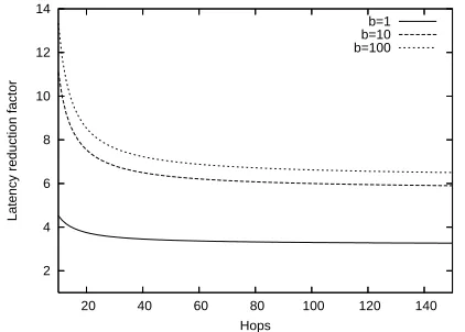
Figure 7 shows a plot of latency gain when the segment length is 10 for various values of b (h
assumed a multiple of 10) using equation 8.
2 4 6 8 10 12 14
20 40 60 80 100 120 140
Latency reduction factor
Hops
b=1 b=10 b=100
Fig. 7. Latency reduction factor of Simple PAC over conventional forwarding for different packet burst lengths.
The latency reduction factor is nearly constant for higher h’s. Noting that (h/Ls)−1 ≤ h/Ls, we
can get a conservative (lower bound) estimate of the latency reduction factor that is independent of h, as
Γconv
pac =
λconv
λpac ≥
656 +b·4288
868 +b·676 + 900+Lbs·3616 (9)
Figure 8 shows a plot againstLsfor various values
of b. As expected, S-PAC does better when the segment length is longer since a packet can be cut-through switched for a longer time before needing to be fully received. At a segment length of 1, the scheme falls back to the conventional scheme (notably, there is no degradation in performance). At reasonable Ls, say 15, there is a 2.5x to 5x
reduc-tion. Note that this analysis is under a single stream so the main advantage of PAC – not having to repeat MAC contention, is not utilized. Given this, it is remarkable that even a very simple protocol like S-PAC achieves significant gains.
One negative feature of Simple PAC is that there may be a significant lag between acquiring the floor and using it. In particular, consider a relay node
R within a single segment path. When it transmits the multi-hop S-RTS, it acquires the floor (blocks its neighbors from transmitting). However, for R
to actually use the acquired floor, that is, transmit DATA, it takes two path roundtrip times during which the neighbors are unnecessarily blocked. In
1 1.5 2 2.5 3 3.5 4 4.5 5 5.5
5 10 15 20 25 30
Latency reduction factor
Segment Length
b=1 b=10 b=100
Fig. 8. Latency reduction factor of Simple PAC over conventional forwarding as a function of segment length.
contrast, in conventional transport, only one hop is reserved at a time and so the wastage is only on the order of the hop roundrip time.
While this does not affect latency performance on a relative basis, the question arises whether there is an impact on relative capacity. To study this comprehensively requires analysis beyond the scope of this paper. Here we present a rough analysis with a view to obtaining insight into the tradeoffs.
To simplify the analysis, we have invented and used the notion of spatial disuse. The spatial disuse
ψf created by a flow f is the total amount of
time that nodes have been blocked from transmitting or receiving packets other than those belonging to flow f. While spatial disuse does not measure capacity or its wastage directly, it is strongly in-versely correlated. In particular, the relative spatial disuse between two schemes can be taken as an inverse measure of relative capacity with reasonable confidence.
We consider a Manhattan grid as in section III-B, with each node being in communication and interference range of eight of its neighbors. A single segment path goes from source S to destination D as shown in Figure XXX. All of the nodes (and only the nodes) in the grid that are affected by this path are shown.
Node M is blocked when A is the receiver of a frame, when A sends the frame again (and B
receives it), when B sends it (and C receives it) and whenC sends it, making a total of 4 handshake times, or 4·T. The blocking times for nodes on the boundary (one hop from the source or destination) are less and are as shown in the figure. The spatial disuse for conventional is given by
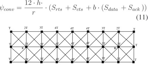
ψconv= (3·(4·(h−3) + 2∗3 + 2∗1))·THconv (10)
where Tconv
H is the time for a handshake of RTS,
CTS, a burst b of DATA-ACK. Denoting the data rate byr, and the sizes asSrts,Scts,SdataandSack,
we haven
ψconv= 12·h·
r ·(Srts +Scts +b·(Sdata +Sack))
(11) T 0 0 1 1 0 0 1 1 00 00 11 11 0 0 1 1 0 0 0 1 1 1 0 0 1 1 00 00 11 11 00 00 11 11 0 0 1 1 0 0 1 1 0 0 1 1 0 0 1 1 0 0 1 1 0 0 1 1 00 00 11 11 0 0 1 1 0 0 1 1 0 0 1 1 00 00 11 11 0 0 1 1 0 0 1 1 0 0 1
1 000
1 1 1 0 0 1 1 0 0 1 1 0 0 1 1 0 0 0 0 0 0 0 0 0 0 0 0 0 0 0 0 0 0 0 0 1 1 1 1 1 1 1 1 1 1 1 1 1 1 1 1 1 1 1 1 0 0 0 0 0 0 0 0 0 0 0 0 0 0 0 0 0 0 0 0 1 1 1 1 1 1 1 1 1 1 1 1 1 1 1 1 1 1 1 1 0000000000 0000000000 0000000000 0000000000 0000000000 0000000000 0000000000 0000000000 0000000000 0000000000 0000000000 0000000000 0000000000 0000000000 0000000000 0000000000 0000000000 0000000000 0000000000 0000000000 1111111111 1111111111 1111111111 1111111111 1111111111 1111111111 1111111111 1111111111 1111111111 1111111111 1111111111 1111111111 1111111111 1111111111 1111111111 1111111111 1111111111 1111111111 1111111111 1111111111 00000000000 00000000000 00000000000 00000000000 00000000000 00000000000 00000000000 00000000000 00000000000 00000000000 00000000000 00000000000 00000000000 00000000000 00000000000 00000000000 00000000000 00000000000 00000000000 00000000000 00000000000 11111111111 11111111111 11111111111 11111111111 11111111111 11111111111 11111111111 11111111111 11111111111 11111111111 11111111111 11111111111 11111111111 11111111111 11111111111 11111111111 11111111111 11111111111 11111111111 11111111111 11111111111 0000000000 0000000000 0000000000 0000000000 0000000000 0000000000 0000000000 0000000000 0000000000 0000000000 0000000000 0000000000 0000000000 0000000000 0000000000 0000000000 0000000000 0000000000 0000000000 0000000000 1111111111 1111111111 1111111111 1111111111 1111111111 1111111111 1111111111 1111111111 1111111111 1111111111 1111111111 1111111111 1111111111 1111111111 1111111111 1111111111 1111111111 1111111111 1111111111 1111111111 0000000000 0000000000 0000000000 0000000000 0000000000 0000000000 0000000000 0000000000 0000000000 0000000000 0000000000 0000000000 0000000000 0000000000 0000000000 0000000000 0000000000 0000000000 0000000000 0000000000 1111111111 1111111111 1111111111 1111111111 1111111111 1111111111 1111111111 1111111111 1111111111 1111111111 1111111111 1111111111 1111111111 1111111111 1111111111 1111111111 1111111111 1111111111 1111111111 1111111111 000000000000 000000000000 000000000000 000000000000 000000000000 000000000000 000000000000 000000000000 000000000000 000000000000 000000000000 000000000000 000000000000 000000000000 000000000000 000000000000 000000000000 000000000000 000000000000 000000000000 000000000000 111111111111 111111111111 111111111111 111111111111 111111111111 111111111111 111111111111 111111111111 111111111111 111111111111 111111111111 111111111111 111111111111 111111111111 111111111111 111111111111 111111111111 111111111111 111111111111 111111111111 111111111111 00000000000 00000000000 00000000000 00000000000 00000000000 00000000000 00000000000 00000000000 00000000000 00000000000 00000000000 00000000000 00000000000 00000000000 00000000000 00000000000 00000000000 00000000000 00000000000 00000000000 00000000000 11111111111 11111111111 11111111111 11111111111 11111111111 11111111111 11111111111 11111111111 11111111111 11111111111 11111111111 11111111111 11111111111 11111111111 11111111111 11111111111 11111111111 11111111111 11111111111 11111111111 11111111111 00000000000 00000000000 00000000000 00000000000 00000000000 00000000000 00000000000 00000000000 00000000000 00000000000 00000000000 00000000000 00000000000 00000000000 00000000000 00000000000 00000000000 00000000000 00000000000 00000000000 00000000000 00000000000 11111111111 11111111111 11111111111 11111111111 11111111111 11111111111 11111111111 11111111111 11111111111 11111111111 11111111111 11111111111 11111111111 11111111111 11111111111 11111111111 11111111111 11111111111 11111111111 11111111111 11111111111 11111111111 000000000000 000000000000 000000000000 000000000000 000000000000 000000000000 000000000000 000000000000 000000000000 000000000000 000000000000 000000000000 000000000000 000000000000 000000000000 000000000000 000000000000 000000000000 000000000000 000000000000 000000000000 111111111111 111111111111 111111111111 111111111111 111111111111 111111111111 111111111111 111111111111 111111111111 111111111111 111111111111 111111111111 111111111111 111111111111 111111111111 111111111111 111111111111 111111111111 111111111111 111111111111 111111111111 00000000000 00000000000 00000000000 00000000000 00000000000 00000000000 00000000000 00000000000 00000000000 00000000000 00000000000 00000000000 00000000000 00000000000 00000000000 00000000000 00000000000 00000000000 00000000000 00000000000 00000000000 11111111111 11111111111 11111111111 11111111111 11111111111 11111111111 11111111111 11111111111 11111111111 11111111111 11111111111 11111111111 11111111111 11111111111 11111111111 11111111111 11111111111 11111111111 11111111111 11111111111 11111111111 00000000000 00000000000 00000000000 00000000000 00000000000 00000000000 00000000000 00000000000 00000000000 00000000000 00000000000 00000000000 00000000000 00000000000 00000000000 00000000000 00000000000 00000000000 00000000000 00000000000 00000000000 11111111111 11111111111 11111111111 11111111111 11111111111 11111111111 11111111111 11111111111 11111111111 11111111111 11111111111 11111111111 11111111111 11111111111 11111111111 11111111111 11111111111 11111111111 11111111111 11111111111 11111111111 00000000000 00000000000 00000000000 00000000000 00000000000 00000000000 00000000000 00000000000 00000000000 00000000000 00000000000 00000000000 00000000000 00000000000 00000000000 00000000000 00000000000 00000000000 00000000000 00000000000 00000000000 11111111111 11111111111 11111111111 11111111111 11111111111 11111111111 11111111111 11111111111 11111111111 11111111111 11111111111 11111111111 11111111111 11111111111 11111111111 11111111111 11111111111 11111111111 11111111111 11111111111 11111111111 00000000000 00000000000 00000000000 00000000000 00000000000 00000000000 00000000000 00000000000 00000000000 00000000000 00000000000 00000000000 00000000000 00000000000 00000000000 00000000000 00000000000 00000000000 00000000000 00000000000 11111111111 11111111111 11111111111 11111111111 11111111111 11111111111 11111111111 11111111111 11111111111 11111111111 11111111111 11111111111 11111111111 11111111111 11111111111 11111111111 11111111111 11111111111 11111111111 11111111111 0000000000 0000000000 0000000000 0000000000 0000000000 0000000000 0000000000 0000000000 0000000000 0000000000 0000000000 0000000000 0000000000 0000000000 0000000000 0000000000 0000000000 0000000000 0000000000 0000000000 1111111111 1111111111 1111111111 1111111111 1111111111 1111111111 1111111111 1111111111 1111111111 1111111111 1111111111 1111111111 1111111111 1111111111 1111111111 1111111111 1111111111 1111111111 1111111111 1111111111 0000000000 0000000000 0000000000 0000000000 0000000000 0000000000 0000000000 0000000000 0000000000 0000000000 0000000000 0000000000 0000000000 0000000000 0000000000 0000000000 0000000000 0000000000 0000000000 0000000000 1111111111 1111111111 1111111111 1111111111 1111111111 1111111111 1111111111 1111111111 1111111111 1111111111 1111111111 1111111111 1111111111 1111111111 1111111111 1111111111 1111111111 1111111111 1111111111 1111111111 S D
T 2T 3T 4T 4T 4T
4T 4T 4T 4T 4T 4T 3T 3T 3T 3T 3T 2T 2T 2T 2T 2T T T T T 0 0 1 1
Fig. 9. Amount of time, in units of T, that each node is blocked from sending, when a packet is sent fromStoDin conventional systems.
Now consider PAC. Consider a node M that is
m hops from the source toward the destination as shown in Figure XXX (b). This node and its neighbors are free until the time the S-RTS from the source reaches M, and busy thereafter. Further, it is busy for a period that is the sum of the time taken for the S-RTS to reach the destination, for the S-CTS to go from the destination to the source, and a burst b of S-DATA and S-ACK to complete. And since there are three such rows, we have
ψpac = 3·(
h
m=1
(h−m+ 1)Srts
r +
(h+ 3)
r (Scts +b·(Sdata +Sack)))
Using size numbers from before, the disuse ratio
is thus
∆pac
conv =
699·(h+ 1) + (3h+ 9)·(290b+ 836)
3624 + 47808b)
(12)
The disuse ratio is plotted in Figure 10.
0 1 2 3 4 5 6 7 8
10 20 30 40 50 60 70 80 90 100
Capacity reduction factor
Hops
b=1 b=10 b=20 Breakeven
Fig. 10. Disuse ratio (Conventional disuse divided by S-PAC disuse. When disuse ratio is less than one, S-PAC is doing better than Conventional in terms of capacity.
Figure 10 shows that there is a tension between the advantage of quickly getting a packet trans-mission completed and the disadvantage of waiting around without utilizing the acquiredfloor. There is a cut-off number of hops beyond which S-PAC has more spatial disuse than conventional. The cut-off point depends upon the burst length b – the more
b is, the higher the hop number at which the S-PAC becomes worse. What is interesting is not that S-PAC wastes capacity (this is intuitively obvious) but that for smaller networks, we can actually get the latency gains without losing capacity gains.
Nonetheless, this calls for more intelligent Path Access Control, where the DATA packet might follow the S-RTS rather than wait for the S-CTS. This idea, termed tailgating PAC is under research.
IV. EXPERIMENTALANALYSIS
We have implemented a simulation model for the ultra low latency system described in the previous section using NS-2 (version 2.28) [14]. We chose NS-2 due to its relative ease of use. NS-2 is a discrete event simulator whose source code is split between C++ for core implementation and OTcl for configuration and scripting. NS-2 supports wireless networks such as MANETs and Wireless LANs and its implementation includes an 802.11 module.
two major changes to the source code. The first change is for S-PAC and enables multihop support of 802.11 MAC frames. That is, we augmented the RTS,CTS,DATA,ACK frames with a target destina-tion field. On the transmission path of the 802.11 MAC, we inserted appropriate hooks to allow the update of relevant frame fields, and to allow access to the forwarding table at each hop. On the reception path, intermediate hops can relay any 802.11 MAC frame while only segment termination nodes can generate CTS and ACK frames.
The second change is for the ROPL in which pipelining of frame bits occurs. In our model, when thefirst bit of frame is detected by the WirelessPHY module, the entire frame is retrieved and forwarded after a delay equivalent to the time to transmit an RTS-sized block. A two-orthogonal-channel model (one channel for control traffic and another for data) has been added to support ROPL. All frames are transmitted based on information contained in the
transit table. The transit table is an array (indexed by source and destination) of keep/relay/discard
enumerations and is populated based on information learnt through 802.11 frames and/or the forwarding table. For carrier sensing to work effectively in our PAC-enabled environment, the NAV duration has been set to a function of the number of hops and transmit times of RTS and DATA frames.
With the aforementioned NS-2 changes, an in-stance of a multihop wireless mesh network is created by placing a set of N2 nodes in a N x N
square area. Nodes are stationary and are placed in a Manhattan grid. Routes among nodes are statically configured with the help of a NO Ad-Hoc Routing Agent (NOAH) [15]. In all our experiments, we assume a channel rate of 11Mbps for both 802.11 and S-PAC. We have experimented with two modes of PHY operation using S-PAC. The first mode is ROPL while the second mode is the conventional 802.11 PHY in which the entire packet is received by the PHY, passed to upper layers (including Routing) before possible re-contention on the same channel. For traffic generation, a fraction p of all nodes are selected randomly to be sources of traffic while nodes, not too close from sources, are picked randomly as destinations. Each source can generate CBR traffic at a rate of R packets per second. To speed up simulations, we use longer packets (of
8000 bits in base size) instead of many packets. This abstractly models back-to-back packet transmissions within RTS/CTS round trips. Each simulation lasts
S seconds. A traffic session starts at a time uni-formly distributed between 1 and(S−2D)seconds and lasts for a duration uniformly distributed around
D seconds (namely [0.8D,1.2D]).
A. PAC Performance
We now analyze the performance of PAC versus that of 802.11 as a function of the network size and the offered load. Both aforementioned PHY modes are considered for PAC. In all our experiments,
(R, D, S) = (1,50,200)11. Metrics of particular
interest are
• Latency: The end-to-end delay of the applica-tion traffic.
• Average number of segments: The total number of segments per path over total number of paths. In all cases considered, the packet delivery rate is 100 %.
Figure (11) depicts the latency as a function of the number of hops for a single traffic flow (no contention). In this experiment, 802.11 has been considered with and without use of RTS/CTS. Not surprisingly, PAC outperforms both 802.11 cases by at least a factor of 4. This result confirms our numerical analysis.
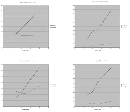
For the remaining section, we shall consider that RTS,CTS frames are always in use with 802.11. Figure (12) shows a set of results with multiple traffic flows (p = 12%). In all associated figures, the latency is depicted as a function of the network size for various rates of flow and packet burst. PAC still outperforms 802.11 but the gap increases sig-nificantly with an increased traffic burst. Overall we obtain 3.5x to 8x gain (depending upon burstiness) at moderate, and realistic loads. Gains are higher with smaller number of higher-rate flows than with a larger number of lower-rate flows. analysis.
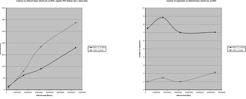
Figure (13) shows results with PAC operating on top of a conventional PHY. Unlike earlier figures, the X axis has offered load rather than number of hops befause of the difficulty in controlling the number of hops per flow while preserving random-ness. Without ROPL, PAC does slightly worse than
Simple PAC vs 802.11/CSMA (1 flow)
0 20 40 60 80 100 120
0 5 10 15 20 25 30 35 40 45 50
number of hops
la
ten
cy (m
sec) Simple PAC
802.11 (+RCDA) 802.11
Fig. 11. Singleflow (one source to one destination), relay-oriented PHY.
latency vs N, p=12%, burst = 1pkt
0 5 10 15 20 25 30 35 40
0 5 10 15 20 25
N (mesh of NxN)
802.11 PAC
latency vs N, p = 12%, burst = 32 pkts
0 50 100 150 200 250 300 350 400 450 500
0 5 10 15 20 25
N (mesh of NxN)
802.11 PAC
latency vs N, p=20%, burst = 1 pkt
0 5 10 15 20 25 30 35
0 5 10 15 20 25
N (mesh of NxN)
802.11 PAC
latency vs N, p =20%, burst = 32 pkts
0 50 100 150 200 250 300 350 400 450
0 5 10 15 20 25
N (mesh of NxN)
802.11 PAC
Fig. 12. Multipleflows (many source-destination pairs) with various bursts, relay-oriented PHY.
802.11 in terms of latency. Indeed all PAC frames now have to re-contend for channel access at each hop, which increases the per-hop delay. This result shows that PAC must be used in conjunction with ROPL to obtain maximal gains.
V. IMPLEMENTATIONCONSIDERATIONS
Latency vs offered load, 10x10 net, p=20%, regular PHY (block size = data size)
0 50 100 150 200 250 300 350
0 10000000 20000000 30000000 40000000 50000000 60000000 70000000
offered load (B/sec)
la
te
n
cy(
msec) 802.11, p=20%
PAC, p=20%
number of segments vs offered load, 10x10 net, p=20%
0 1 2 3 4 5 6 7 8 9 10
0 10000000 20000000 30000000 40000000 50000000 60000000 70000000
offered load (B/s)
num
be
r of
s
e
g
m
e
nt
s
802.11, p=20% PAC, p=20%
Fig. 13. Multipleflows (many source-destination pairs), conventional PHY.
In this section, we show why this is not as hard as it may appear. First, as noted earlier, the ROPL does not involve any changes in the signal processing elements in the receive or transmit chain. Given any legacy physical layer RF and modem compo-nents, ROPL simply adds processing at the end of the receive chain and at the head of the transmit chain. Thus, if there is an on-board CPU, simple code can be written to implement the algorithm described in section III-A. Alternatively, one can use a Field Programmable Gate Array (FPGA) into which the logic is burnt in. The floor state and the relay table are loaded into the FPGA as and when they change. If the transmit and receive processing (modem functions) are part of an existing FPGA whose source code (e.g. Verilog) is available, they can be upgraded with the same logic. Thus it is relatively easy for a chipset manufacturer (such as Atheros), or even a wireless LAN card vendor (such as Cisco) to build an ROPL.
A more exciting and flexible avenue is through the use of a software radio. A software radio gets code as close to the antenna as possible [17]. In contrast to conventional radios which processing is done using analog circuitry and digital chips, in a software radio the software defines the trans-mitted waveforms and demodulates the received waveforms. Software radios are beginning to find increasing usage both in the military and commer-cial [16] worlds.
We consider a design based on the open source GNU Software Radio [17]. While this is currently
not fully capable of full-fledged packet based com-munications and protocols, work is underway that will make it a viable platform for hosting MANET-like protocols. Specifically, the DARPA ACERT program is investing heavily in the GNU Radio to make it usable by researchers. It will have a full digital transceiver and a flexible MAC protocol. Given these, to upgrade to an ROPL is simply a question of additional code.
The Gnu Radio architecture is based upon a number of processing blocks written in C++ that are strung together in real-time using the Python lan-guage. The processing blocks perform such receive functions as demodulation, decoding, descrambling etc. and transmit functions such as modulation, cod-ing, scrambling etc. When a block B1 is connected
to block B2, the bit stream that is out put from B1
becomes the input stream for B2 on which it acts.
implemented on the daughterboards.
New
Rcv Front End
Xmt Front End ADC
DAC
GNU Radio Existing Blocks (Rcv)
GNU Radio Existing Blocks (Xmt) Mem with tables
USRP
block
Fig. 14. Implementation outline of ROPL using GNU Radio
The implementation sketch for ROPL using the GNU Radio is given in Figure 14. The solution consists of creating a new processing block (called
relay processing, and having the output of the last processing block in the receive chain be connected to the input of relay processing and the output of
relay processing be connected to the first block in the transmit chain. The relay processing block reads the header, looks up the routing tables in the memory, decides whether or not to relay and activates the sending of the stream, as was discussed in more detail in section III-A. Writing a new block is relatively easy by inheriting from gr block class, and is described in [19].
The PAC is, of course, not so hard to imple-ment even in conventional hardware, but is even more easy in Gnu Radio environment. Under the aforementioned DARPA ACERT project, common elements needed for MAC are being built and can easily be adapted for PAC.
VI. CONCLUDINGREMARKS
If current trends in MANET topologies and real-time applications continue, the ability of conven-tional MANET mechanisms to support the end-to-end latency requirements of applications will be under serious threat. Incremental advances in MAC and network layer will be insufficient to provide the dramatic reduction in latency that is required.
We have described two key components of a solution for ultra low latency packet transport in MANETs. Our Relay-Oriented Physical Layer (ROPL) performs cut-through switching using or-thogonal frequencies for transmit and receive, and by pipelining the received bits as soon as the first few bytes of the packet are received and a decision
is made on relaying. A proactive routing protocol injects next-hop forwarding table information into the physical layer. The ROPL cuts the switching time by a factor of more than 10x at expected data rates and packet size.
We also described S-PAC – a simple mechanism for path access control. S-PAC extends the hop-oriented RTS/CTS/DATA/ACK handshake to a path oriented regime. It works in units of segments, multiple segments constituting an end-to-end path. The S-PAC terminates and re-initates segments, allows packet bursts, assigns frequencies and creates
sentinel nodes for protecting the transfer. Simple numerical analysis shows that the S-PAC reduces the end-to-end latency by more than a factor of 5, and may even increase the capacity upto a certain number of hops.
Using NS-2, we have conducted experiments on an abstract model of the ROPL and S-PAC on a Manhattan grid topology with random streams of traffic. Our simulations show a gain of 3.5x to 8x in latency over the baseline.
A number of exciting research directions need to be explored. The S-PAC, while simple, has a number of obvious inefficiencies that can be removed. New path access control mechansims where the DATA packet does not have to wait at the source till the RTS/CTS is complete also need to be inves-tigated. TDMA-oriented PAC is another promising but unexplored direction. The concept of adaptively controlling the segment length based on error and other characteristics is a challenging yet fruitful topic. Finally, implementing the ROPL and the PAC into a prototype testbed, either using conventional hardware or the GNU Radio will be the ultimate validation of this concept.
REFERENCES [1] http://www.darpa.mil/ato/solicit/WANN/index.htm
[2] J. M. Kahn and R. H. Katz and K. S. J. Pister, “Next century challenges: mobile networking for smart dust”,Proc. ACM MobiCom, 1999. [3] J. Bicket, D. Aguayo, S. Biswas, R. Morris, “Architecture and Evaluation
of an Unplanned 802.11b Mesh Network”,Proc. ACM Mobicom, 2005. [4] R. Ramanathan, “Challenges: A Radically New Architecture for Next
Generation Mobile Ad Hoc Networks,”Proc. ACM Mobicom, 2005. [5] http://www.darpa.mil/ipto/Programs/acert/index.htm
[6] M.S. Gast, e Definitive Guide”, O’Reilly and Associates, April 2002. [7] P. Kermani and L. Kleinrock, “Virtual Cut-through: A New Computer
Communication Switching Technique”, Computer Networks, 3(3):267– 286, September 1979.
[9] A. Acharya, A. Misra, and S. Bansal, “A Label-switching Packet Forwarding Architecture for Multi-hop Wireless LANs,”IBM Tech. Rep., 2002.
[10] D. Raguin, M. Kubisch, H. Karl, A. Wolisz, “Queue-Driven Cut-through Medium Access in Wireless Ad Hoc Networks”IEEE Wireless Commu-nications and Networking Conference (WCNC), Atlanta, Georgia, USA, March 2000
[11] P. Jacquet, P. Muhlethaler, and A. Quayyum, “Optimized link state routing protocol”, IETF MANET Working Group Internet-Draft, Work in Progress
[12] C. Santivanez, S. Ramanathan, I. Stavrakakis, “Making Link State Routing Scale for Ad Hoc Networks,” in Proc. ACM MobiHocLong Beach, CA, Oct. 2001.
[13] B. Sadeghi, V. Kanodia, A. Sabharwal, E. Knightly, “OAR: An Op-portunistic Auto-rate Media Access Protocol for Ad Hoc Networks”
Wireless Networks, Vol 11, Nos 1-2, Jan 2005
[14] The Network Simulator, NS-2. http://www.isi.edu/nsnam/ns. [15] NO AdHoc Routing Agent (NOAH).
http://icapeople.epfl.ch/widmer/uwb/ns-2/noah/ [16] Vanu Inc. http://www.vanu.com