Symmetrical Trapezoidal Normal Distribution and its Parameter Estimation

(1)

Vol. 20, No. 1, 2019, 35-47

ISSN: 2279-087X (P), 2279-0888(online) Published on 11 September 2019

www.researchmathsci.org

DOI: http://dx.doi.org/10.22457/apam.623v20n1a6

35

Annals of

Symmetrical Trapezoidal Normal Distribution

and its Parameter Estimation

Soontorn Boonta1 and Somchit Boonthiem2

1

Department of General Science, Kasetsart University

Sakon Nakhon 47000, Thailand. E-mail: soontorn.bo@ku.th

2

Mathematics and Statistics Program, Sakon Nakhon Rajabhat University, Sakon Nakhon 47000, Thailand. E-mail: somchit_math@snru.ac.th

Received 20 July 2019; accepted 2 September 2019

Abstract. The trapezoidal rule is applied for construction a new distribution based on normal distribution, is called trapezoidal normal distribution under the same conditions. Furthermore, we illustrate the parameter estimation of the trapezoidal normal distribution using standard differential evolution (DE) algorithm for the sample sizes equal to 10 to 100. The results show the K-S statistic of the trapezoidal normal distribution is less than the K-S statistic of the normal distribution of each sample size data.

Keywords: Trapezoidal normal distribution, Differential evolution algorithm. AMS Mathematics Subject Classification (2019): 62F10

1. Introduction

Normal distribution is one of the most important continuous probability distribution which is widely used in statistical analysis and other fields such as biology, economics, engineering, and so forth. The random variable X is called a normal distribution with the real location parameter µ and the positive scale parameterσ, denoted by

(

2

)

,

X ∼N µ σ

and its probability density function is of the form

(

)

2

1 2

1

; , , .

2 x

X x e x

µ σ

φ µ σ

σ π

−

 

− _ _

= ∈ℝ

The cumulative distribution function is of the form

(

; ,

)

x

(

; ,

)

.

X X

F x µ σ φ x µ σ dx

−∞

=

_∫

(2)

36

used to join exponential distribution and to determine the inefficiency level of the firms due to the effect of exogenous factors [5]. Furthermore, a few researchers studied some properties of generalized trapezoidal distribution and its applications which triangular and uniform distributions are special cases of the trapezoidal family. Van Dorp and Kotz [6] allows for a non-linear behavior at its tails and a linear incline (or decline) in the central stage and another. Van Dorp et al. [7] developed two novel elicitation procedures for the parameters of a special case of the generalized trapezoidal family by restricting ourselves to a uniform (horizontal) central stage in accordance with the central stage of the original trapezoidal distribution.

In this paper, we shall introduce a new distribution based on normal distribution which is called trapezoidal normal distribution by applying trapezoidal rule.

2. Definitions and main theorems

We propose definition, theorem and corollary that relate to the probability density function g x

(

; ,Ρφ

)

in case of 2n+1 nodes and 2n+2 nodes.

Definition 1. Let k≥3 be an integer, ℓ,d>0_{be real numbers. A set}

{

}

1, 2, , k

x x x

Ρ = …

is called a

(

k x, , ,1 ℓ d

)

node if x1<x2< <⋯ xk such that x2− =x1 xk −xk−1=ℓ and

1 ,

i i

x₊ − =x d i=2,3,…,k−2.

The node Ρis denoted by the notationNode k x

(

, , ,1 ℓ d

)

.

Remark 1. Let k≥3 be an integer, ℓ,d>0_{be real numbers.}

1.1 If Ρbe a

(

k x, , ,1 ℓ d

)

node, x2= +x1 ℓ, xk = +x1 2ℓ+ −

(

k 3

)

d and

( )

1 1 1 ,

i

x₊ = + + −x ℓ i d _where_i=_2,3,…_,_k−_2.

1.2 Let f be a function and I be the identity function on Ρ,we denote ∆f x

( )

k = f x

( ) ( )

k − f xk−1

∆x_k = ∆I x

( )

_k =x_k −x_k₋₁

f x

( )

_k

(

( ) ( )

1

)

1

2 f xk f xk−

= +

x k

( )

(

1

)

1

. 2

k k k

I x x x ₋

= = +

Remark 2. Let k≥3,n≥1 be integers, ℓ,d>0_{be real numbers and}_C_{be a center node.}

2.1 CeNode

(

2n+2, , ,C ℓ d

)

₂ _2, 1 _{, ,}

2

Node n C n d d

=  + − −  − 

 

(3)

37

Theorem 3. Let µ∈ℝ,σ >0,d>0,n∈ℕ,φ_{be a probability density function} of

(

2

)

,

N µ σ , and Ρ =

{

x x₁, ₂,…,x₂_n₊₁

}

_be_CoNode

(

₂_n+_{1, , ,}µ ℓ _d

)

_{. If}

( )

2 3 0 1 n k k x d φ =

<

∑

< ,

( )

2 3 2 1 1 n k k x d x φ φ =   =  −  

∑



ℓ _and

(

; ,

)

g x Ρφ

( ) ( )(

)

( )

( )(

)

( ) ( )(

)

2

2 2 1 2

1

2

2 2 2 2 1

; ,

; , 3, 4, , 2

; , k

k k k k

n

n n n n

x

x x x x x x

x

x x x x x x k n

d x

x x x x x x

φ φ φ φ φ φ − + 

+ − < ≤

 

∆ 

= + − < ≤ =

 

− − < ≤

  ℓ … ℓ (1)

when the other of g x

(

; ,Ρφ

)

is zero. Then g x

(

; ,Ρφ

)

is a probability density function.

Proof: We will show that g x

(

; ,Ρφ

)

≥0 for all x∈ℝ and ∞ g x

(

; ,φ

)

dx 1

−∞ Ρ =

∫

.

Since φ

( )

x is increasing on

[

x x1, n+1

]

and φ

( )

x is decreasing on

[

xn+1,x2n+1

]

,

(

; ,

)

0

g x Ρφ ≥ for all x . Next, we consider

(

)

2 1

(

)

1

; , xn ; ,

x

g x φ dx + g x φ dx

∞

−∞ Ρ = Ρ

∫

so we

have

(

; ,

)

g x φ dx

∞ −∞ Ρ

∫

2

(

)

(

)

2 1

(

)

1 1 2

2

3

; , k ; , n ; ,

k n

n

x x x

k

g x φ dx g x φ dx + g x φ dx

− = =

∫

Ρ +

∑

∫

Ρ +

∫

Ρ

( )

2 2 2 3 2 2 n n k k x x x d φ _φ φ = = ℓ+

∑

+ ℓ

( )

2 2 2 3 2 2 n k k x x x d φ _φ φ = = ℓ+

∑

+ ℓ

( )

2 2 3 . n k k

x x d

φ φ = = ℓ+

∑

Since

( )

2 3 2 1 1 n k k x d x φ φ =   = _ − _ 

∑



ℓ is an appropriate value,

(

)

(

)

2 1

1

; , 1 ; ,

n x

x g x φ dx g x φ dx

+ ∞

−∞

Ρ = = Ρ

∫

(4)

38

Theorem 4. Let µ∈ℝ,σ >0,d>0,n∈ℕ,φ_{be a probability density function of}

(

2

)

,

N µ σ , and Ρ =

{

x x1, 2,…,x2n+2

}

be CeNode

(

2n+2, , ,µ ℓ d

)

. If

( )

2 1

3

0 1

n k k

x d

φ

+ =

<

∑

< ,

( )

2 1

3 2

1 1

n k k

x d

x φ

φ

+ =

 

= _ − _



∑



ℓ _and

(

; ,

)

g xΡφ

( ) ( )(

)

( )

( )(

)

(

) (

)(

)

2

2 2 1 2

1

2 1

2 1 2 1 2 1 2 2

; ,

; , 3, 4, , 2 1

; , k

k k k k

n

n n n n

x

x x x x x x

x

x x x x x x k n

d x

x x x x x x

φ φ

− +

+ + + +



+ − < ≤

 

∆ 

= + − < ≤ = +

 

− − < ≤

 

ℓ

…

ℓ

(2)

when the other of g x

(

; ,Ρφ

)

is zero. Theng x

(

; ,Ρφ

)

is a probability density function.

Proof: The proof of Theorem 4 follows from Theorem 3.

Definition 2. The random variable X has trapezoidal-normal distribution for parameters

(

µ σ,

)

such that µ ∈ℝ and σ >0 corresponding to Conode

(

2n+1, , ,µ ℓ d

)

or

(

2 2, , ,

)

Cenode n+ µ ℓ d _{denoted by}

(

2

)

, , ,

X ∼TN µ σ n Ρ _{, if there exists a probability}

density function satisfying equations (1) and (2), respectively.

Definition 3. A probability distribution is said to be symmetric if and only if there exists a value x such that 0 f x

(

0−δ

)

= f x

(

0+δ

)

for all real number δ,where f is the

probability density function if the distribution is continuous or the probability mass function if the distribution is discrete.

Theorem 5. Let g x

(

; ,Ρφ

)

be the probability density function of trapezoidal-normal distribution for parameters

(

µ σ,

)

,

(

; ,

) (

; ,

)

g µ− Ρx φ =g µ+ Ρx φ

for all real number x , g x

(

; ,Ρφ

)

is called symmetric.

Proof: Let x∈

[

x xk, k+1

]

for all x∈ℝ. Let x lie in a segment that has the first point,

( )

(

xk,φ xk

)

and the end point,

(

xk+1,φ

( )

xk+1

)

. We have a straight line equation in the

(5)

39

( )

( )(

1

) ( )

1

k

k k k

k

x

y x x x x

x

φ

+ +

∆

= − +

∆ .

Since φ

( )

x is symmetry,

(

x

) (

x

)

φ µ− =φ µ+ .

We will show that g

(

µ+ Ρx; ,φ

) (

=g µ− Ρx; ,φ

)

. Here, we consider only 5 cases of odd node and similarity to consider of even node:

Case 1. For µ+ <x x1, we get µ− >x x2n+1.

Since µ− >x 2µ− =x₁ x₂_n₊₁, we have g

(

µ+ Ρx; ,φ

)

=0 and g

(

µ− Ρx; ,φ

)

=0. Thus, g

(

µ+ Ρx; ,φ

) (

=g µ− Ρx; ,φ

)

.

Case 2. For µ+ >x x2n+1, by similar process as in Case 1, we get

(

; ,

)

(

( )

; ,

)

(

; ,

)

g µ+ Ρx φ =g µ− −x Ρφ =g µ− Ρx φ

Case 3. For x1< + <µ x x2, we get

(

µ+x g,

(

µ+ Ρx; ,φ

)

lie in a segment that has a

straight line equation

( )

(

2

)

(

) ( )(

2

)

1 1 1

2

; ,

g x x

y x g x x x

x

φ _φ φ

∆ Ρ

= + Ρ = −

∆ ℓ

Thus,

(

)

(

) ( )(

2

) ( )(

2

) ( )

1 1 2 2

; , x x

g µ+ Ρx φ =y µ+x =φ µ+ −x x =φ µ+ −x x +φ x

ℓ ℓ

Conversely, we consider for x₂_n< − <µ x x₂_n₊₁, we get

(

µ−x g,

(

µ− Ρx; ,φ

)

lie in segment that has straight line equation

( )

(

2 1

)(

) (

)

( )(

2

) ( )

2 2 2 2 2

2 1

; ,

n n

n n n n n

n

g x x

y x x x g x x x x

x

φ φ

+ +

∆ Ρ

= + + Ρ = − − +

∆ ℓ

Thus,

g

(

µ− Ρx; ,φ

)

=y_2n

(

µ−x

)

= −φ

( )(

x2n µ− −x x₂_n

) ( )

+φ x₂_n

ℓ

=φ

( )(

x2 µ+ −x x₂

) ( )

+φ x₂

ℓ .

Therefore, g

(

µ+ Ρx; ,φ

)

=g

(

µ− Ρx; ,φ

)

.

Case 4. For x2n< + <µ x x2n+1, by similar process as in Case 3, we have

(

)

(

µ+x g, µ+ Ρx; ,φ

)

lie in a segment that has a straight line equation

( )

(

2 1

)(

) (

)

( )(

2

) ( )

2 2 2 2 2

2 1

; ,

n n

n n n n n

n

g x x

y x x x g x x x x

x

φ φ

+ +

∆ Ρ

= − + Ρ = − − +

(6)

40

thus g

(

µ+ Ρx; ,φ

)

=y2n

(

µ+x

)

( )(

2 2

) ( )

2

n

n n

x

x x x

φ

µ φ

= − + − +

ℓ

( )(

2

) ( )

2 2

x

x x x

φ _µ _φ

= − + +

ℓ .

Conversely, we consider for x₁< − <µ x x₂, we have

(

µ+x g,

(

µ+ Ρx; ,φ

)

lie in segment that has straight line equation

( )

(

2

)( ) (

) ( )(

2

)

1 1 1 1

2

; ,

g x x

y x x x g x x x

x φ φ φ ∆ Ρ = − + Ρ = − ∆ ℓ , thus

(

)

(

) ( )(

2

) ( )(

2

) ( )

1 1 2 2

; , x x

g µ− Ρx φ =y µ− =x φ µ− −x x =φ µ− −x x +φ x

ℓ ℓ .

Therefore, g

(

µ− Ρx; ,φ

)

=g

(

µ+ Ρx; ,φ

)

.

Case 5. For xk < + <µ x xk+1and k=2,3,…, 2n−1, we have

(

µ+x g,

(

µ+ Ρx; ,φ

)

lie in

segments that have straight line equations

( )

(

1

)(

) (

)

( )(

1

) ( )

1 1

; ,

k k

k k k k k

k k

g x x

y x x x g x x x x

x x φ φ φ φ + + + + ∆ Ρ ∆ = − + Ρ = − + ∆ ∆ ,

thus g

(

µ+ Ρx; ,φ

)

=yk

(

µ+x

)

( )(

) ( )

1 1 k k k k x

x x x

x φ µ φ + + ∆ = + − + ∆ .

Consider g

(

µ− Ρx; ,φ

)

=yk

(

µ−x

)

(

2 4

)(

) (

)

2 3 2 3

2 4

n k

n k n k

n k x

x x x

x φ µ φ − + − + − + − + ∆ = − − + ∆

( )(

1

) ( )

1

k

k k

k x

x x x

x φ µ φ + + ∆ = + − + ∆ .

Therefore, g

(

µ+ Ρx; ,φ

)

=g

(

µ− Ρx; ,φ

)

.

The proof is complete.

Theorem 6. Let µ∈ℝ,σ >0,d>0,n∈ℕ,φ_{be a probability density function of}

(

2

)

,

N µ σ , and Ρ =

{

x x₁, ₂,…,x₂_n₊₁

}

_be_CoNode

(

₂_n+_{1, , ,}µ ℓ _d

)

_{. If}

( )

2 3 0 1 n k k x d φ =

<

∑

< ,

( )

2 3 2 1 1 n k k x d x φ φ =   =  −  

∑



ℓ _,

( )

_max

{

_:

}

k

N t = k x ≤t , G x

(

; ,φ

)

x g s

(

; ,φ

)

ds

−∞

(7)

41

(

; ,

)

G x Ρφ

( )(

) ( )

(

)

( )

_{( )}

(

_{( )}

)

( ) ( )

( )

( ) ( ) 1 2 2 2 1

2 1 2 1 1 2

1

3

2 2

1

0 ; , ; , 2

2 N x

k N x N x

k

N x N x

N x

x x

x x x

x x x x x x x x x

x d x x x

x x x

x x d φ φ φ φ φ − = − ≤  ₋ 

− +  − −  < ≤

  + − = _∆ − + − −

∑

ℓ ( )

(

)

( )(

) ( )

(

)

2 2 1 2 2 2 2

2 2 2 2 2 2 1,

2 1

; ,

; 2

1 ; , n N x

n n

n n n n n n

n

x x x x

x x x

x x x x x x x x x

x x φ φ − + +          _ _

 _ _ _{< ≤}

 _ _

 



 _ ₋ _

 ₋ ₋ _ ₋ ₋ _ _{< <}

 _ _  ≥  ℓ

then G x

(

; ,Ρφ

)

is called the cumulative distribution function.

Proof: By using Theorem 3, we get obviously

(

)

(

)

1

2 1

; , 0 ; ,

n x

x

g x φ dx g x φ dx

+

∞

−∞ Ρ = = Ρ

∫

.

We consider in case of x₁< <x x₂,

G x x x

(

;

(

₁, ₂

)

,φ

)

x g s x x

(

;

(

₁, ₂

)

,φ

)

ds

−∞

=

_∫

x φ

( ) ( )(

x₂ φ x2 s x₂

)

ds

−∞   =  + −   

∫

_ℓ

( )(

) ( )

(

)

2 2 2 1

2 1 2 1

2 2

x x x

x x x φ x x x

φ  − 

= − +  − − 

 

ℓ .

For x=x2, we get

(

)

(

)

( )

2

1 2

; , , .

2

x

G x x x φ =φ ℓ

Next, we consider in case of x_k₋₁< <x x_k, k=3, 4,…, 2n_{and since}

( )

max

{

: k

}

N t = k x ≤t , so we get

(

)

(

; 2, 2n ,

)

G x x x φ

(

)

2

2 2

; , ,

x

n

x g s x x φ ds

=

_∫

( ) ( )(

)

2 x k k k x x

x s x ds

d φ φ   =  + −   

∫

( )

( ) ( )

( )

(

( )

)

1 3 N x

k N x N x

k

x d x x x

φ φ

− =

(8)

42

( )

( ) ( ) _{( )}

(

_{( )}

)

2 2 1 1 2

N x N x

x x x

d φ ₋ − ∆  ₋   ₋ ₋      . For all x=x_k, k=3, 4,…, 2n, we get

(

)

(

; 2, 2n ,

)

G x x x φ

( )

2 3 n k k x d φ = =

∑

.

Next, we consider in case of x2n< <x x2n+1,

(

)

(

; 2n, 2n 1 ,

)

G x x x ₊ φ

(

)

2

2 2 1

; , ,

n x

n n

x g s x x + φ ds

=

_∫

( ) ( )(

)

2 2 2 2 x _n n n x x

x φ s x ds

φ   =  − −   

∫

_ℓ

( )(

) ( )

(

)

2 2 2 2

2

n n

n n n n

x x x

x x x φ x x x

φ  − 

= − −  − − 

 

ℓ .

For all x=x2n+1, we get

(

)

(

; 2n, 2n1 ,

)

G x x x ₊ φ

( )

2

2 n

x

φ

= ℓ_.

We combine all cases of x∈

(

x x1, 2n+1

)

, and since

( )

2 3 2 1 1 n k k x d x φ φ =   =  −  

∑

 ℓ _, consequently,

(

; ,

)

g x φ dx

∞ −∞ Ρ

∫

( )

2 2

( )

2

3 1. 2 2 n n k k x x x d φ φ φ = = ℓ+

∑

+ ℓ=

The proof is complete. □ Theorem 7. Let µ∈ℝ,σ >0,d>0,n∈ℕ,φ_{be a probability density function of}

(

2

)

,

N µ σ , and Ρ =

{

x x₁, ₂,…,x₂_n₊₂

}

_be_CeNode

(

₂_n+_{2, , ,}µ ℓ _d

)

_{. If}

( )

2 1 3 0 1 n k k x d φ + =

<

∑

< ,

( )

2 1 3 2 1 1 n k k x d x φ φ + =   = _ − _ 

∑



ℓ _,

( )

_max

{

_:

}

k

N t = k x ≤t , G x

(

; ,φ

)

x g s

(

; ,φ

)

ds

−∞

(9)

43

(

; ,

)

G x Ρφ

( )(

) ( )

(

)

( )

(

( )

)

1

2 2

2 1

2 1 2 1 1 2

0 ; , ; , 2

k N x N x

x x

x x x

x x x x x x x x x

x d x x x

φ φ

≤

 ₋ 

− +  − −  < ≤

 

+ −

=

ℓ

( )

(

( )

)

(

)(

) (

)

(

)

1

3

2 2

1

2 2 1

1

2 2

2 1 2 1

2 1 2 1 2 1 2 1 2 1 2 2,

; ,

2

; 2

1 N x

k

N x N x

n N x N x

n n

n n n n n n

x x x

x x x x x x

d

x x x

x x x x x x x x x

φ

φ φ

− =

−

+ −

+ +

+ + + + + +

∆  ₋ 

 

+ _ − − _ < ≤

 

 ₋ 

− −  − −  < <

 

∑

ℓ

2 2

;x x _n₊ . 

              

≥ 

Then G x

(

; ,Ρφ

)

is called the cumulative distribution function.

Proof: The proof of Theorem 7 follows from Theorem 6.

Let X₁∼TN( ,µ σ2)_{be a random variable of trapezoidal-normal distribution, we found} that Pr

(

X₁ ≤M

)

=1, for some M >0, i.e., X1 is a bounded random variable. At the

same time, if X2∼N

(

µ σ, 2

)

is a random variable of normal distribution, we found that

(

2

)

0<Pr X >M <1 for all M >0.

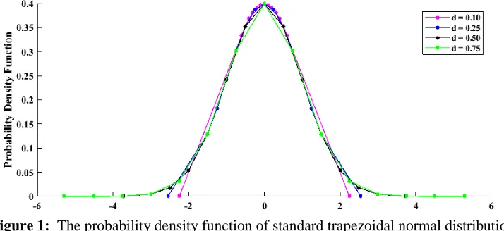
We illustrate the probability density function of trapezoidal-normal distribution, TN

( )

0,1 for n=6 as shown in Figure 1. We can see that the probability density function of different d has also different kurtosis.

(10)

44

Next, we illustrate the probability density function of standard trapezoidal normal distribution, TN

( )

0,1 for n=17, d =0.20(a) and d=0.25 (b) as shown in Figure 2.

(a) (b)

Figure 2: The probability density function of standard trapezoidal normal distribution

3. Parameters estimation method

In this section, we propose a parameter estimation by using standard differential evolution (DE) algorithm. In part of experiment, we random a sample size of standard normal distribution varying from 10 to 100 data (increase by 10) in each test. After that, we approximate parameters using DE algorithm by setting F=2, CR=0.8. The results of these experiments are shown in Table 1 and Table 2. The last figure shows the K-S statistic in some cases.

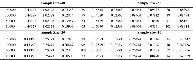
Table 1: The results of parameter estimation of trapezoidal-normal distribution for

2,

F= CR=0.8 by using DE algorithm

Iterations µ σ2 d n K-S

Statistic

µ σ2 d n K-S

Statistic

Sample Size=100 Sample Size=90

150000 0.07930 0.97158 0.01983 93 0.06720 -0.06336 0.95725 0.04793 39 0.06654 100000 0.07930 0.97158 0.05004 31 0.07550 -0.06336 0.95725 0.10366 8 0.05708 50000 0.07930 0.97158 0.01121 19 0.05616 -0.06336 0.95725 0.04055 105 0.06678 10000 0.07930 0.97158 0.00550 24 0.05497 -0.06336 0.95725 0.02598 20 0.06704

150000 0.03236 0.99864 0.04220 38 0.05476 0.04277 1.00452 0.01640 60 0.04798 100000 0.03236 0.99864 0.01021 58 0.04944 0.04277 1.00452 0.01995 50 0.04873 50000 0.03236 0.99864 0.00884 95 0.04787 0.04277 1.00452 0.03388 64 0.05539 10000 0.03236 0.99864 0.00867 41 0.04633 0.04277 1.00452 0.02641 58 0.05187

(11)

45

150000 -0.44127 1.02128 0.04353 70 0.15545 -0.02563 1.09464 0.09477 70 0.08398 100000 -0.44127 1.02128 0.02074 59 0.14520 -0.02563 1.09464 0.07912 48 0.08474 50000 -0.44127 1.02128 0.03457 74 0.15179 -0.02563 1.09464 0.10440 17 0.08161 10000 -0.44127 1.02128 0.03963 63 0.15370 -0.02563 1.09464 0.08341 102 0.08314

150000 0.11367 0.75473 0.01080 39 0.12893 0.10983 0.76474 0.01446 14 0.148247 100000 0.11367 0.75473 0.00847 96 0.12899 0.10983 0.76474 0.01798 10 0.149168 50000 0.11367 0.75473 0.02413 105 0.13761 0.10983 0.76474 0.01105 52 0.147956 10000 0.11367 0.75473 0.00508 33 0.12673 0.10983 0.76474 0.00470 14 0.143389

Table 2: The results of parameter estimation normal distribution for F=2,CR=0.8

by using DE algorithm

Iterations µ σ2 _{K-S Statistic} µ σ2 _{K-S Statistic}

150000 0.22599 0.97165 0.27227 0.00481 1.17743 0.39991 100000 0.27899 0.98001 0.27849 0.18436 1.00489 0.30379

50000 0.11309 0.99637 0.29032 0.09503 0.97272 0.27392

10000 0.39801 0.98497 0.29094 -0.00359 0.96379 0.26686

150000 0.19754 1.02924 0.31309 0.23089 1.07715 0.34367 100000 0.11769 1.02289 0.30878 0.13398 1.02191 0.30813

50000 0.03704 1.00809 0.29861 0.23396 1.04248 0.32184

10000 0.10523 1.07488 0.34222 0.05478 1.01354 0.30240

150000 0.15024 0.94613 0.28936 0.06817 1.08629 0.34906 100000 0.05286 0.93960 0.25572 0.23876 1.02708 0.31154

50000 0.15628 0.97604 0.30893 0.23782 1.02915 0.31292

10000 0.06606 0.99806 0.29799 0.28146 1.05709 0.33109

150000 -0.29152 1.04021 0.35826 0.29018 1.15093 0.39023 100000 -0.41545 1.10236 0.35858 0.34995 1.12379 0.37673 50000 -0.39285 1.02440 0.31591 0.02528 1.11353 0.36658 10000 -0.40140 1.11653 0.36672 0.11752 1.12652 0.37464

150000 0.24826 0.76134 0.22952 0.07190 0.90608 0.24649 100000 0.14258 0.80298 0.21002 0.11593 0.76654 0.18650

50000 0.12668 0.81678 0.21297 0.19940 0.81705 0.25883

10000 0.06381 0.82125 0.18932 0.13269 0.92577 0.28197

(12)

46

(c) (d)

Figure 3: K-S statistic of normal distribution (ND) and trapezoidal normal distribution (TND) for 10,000 iterations (c) and 50,000 iterations (d).

4. Conclusions and recommendations

This research presents the approach to construct the trapezoidal normal distribution. We obtain that its properties are similar to the normal distribution, but trapezoidal normal distribution has bounded, i.e., Pr(X <M) 1= for some M >0 such that it explains some situations better than the normal distribution.

In the future, we will compare the normal distribution with the trapezoidal-normal distribution through parameter estimator. In order to show that it is credible and useful for data analysis as well as the normal distribution. Moreover, we will study trapezoidal-normal distribution and its application for a real world situation. In addition, we should compare our algorithm with other algorithms such as Particle Swarm Optimization algorithm [8] or fuzzy number to reverse order trapezoidal [9].

Acknowledgement. This research was partially supported by Mathematics and Statistics Program, Sakon Nakhon Rajabhat University and Department of General Science, Kasetsart University, Chalermphrakiat Sakon Nakhon Province Campus, Thailand. Moreover, we are very grateful to the referees for their valuable suggestions to improve this research in its present form.

REFERENCES

1. S.R.Bowling, M.T.Khasawneh, S.Kaewkuekool and B.R.Cho, A logistic approximation to the cumulative normal distribution, Journal of Industrial Engineering and Management, 2(1) (2009) 114 – 127.

2. M.Kiani, J.Panaretos, S.Psarakis and M.Saleem, Approximations to the normal function and an extended table for the mean range of the normal variables, Journal of the Iranian Statistical Society, 7(1) (2008) 57 – 72.

3. C.R.Kikawa, M.Y.Shatalov, P.H.Kloppers and A.C.Mkolesia, On the estimation of a univariate gaussian distribution: A Comparative Approach, Open Journal of Statistics, 5 (2015) 445 – 454.

(13)

47

5. S.H.Khan and M.Louis.L, Normal Exponential exogenous model and its application,

Annals of Pure and Applied Mathematics, 16(1) (2018) 235 – 239.

6. J.R.Van Drop, and S.Kotz, Generalized trapezoidal distributions, Metrika, 58 (2003) 85 – 97.

7. J.R.Van Dorp, S.C.Rambaud, J.G.Pérez and R.H.Pleguezuelo, An elicitation procedure for the generalized trapezoidal distribution with a uniform central stage,

Decision Analysis Journal, 4 (2007) 156 – 166.

8. D.K.Biswas and S.C.Panja, Advanced optimization technique, Annals of Pure and

Applied Mathematics, 5(1)(2013) 82 – 89.

9. T.Pathinathan1 and K.Ponnivalavan, Reverse order triangular, trapezoidal and