Adaptive, transparent frequency and voltage scaling of communication phases in MPI programs

(1)

Adaptive, Transparent Frequency and Voltage Scaling of

Communication Phases in MPI Programs

∗

Min Yeol Lim† Vincent W. Freeh∗ David K. Lowenthal‡

Abstract

Although users of high-performance computing are most interested in raw performance, both energy and power consumption have become critical concerns. Some microprocessors allow frequency and voltage scaling, which enables a system to reduce CPU per-formance and power when the CPU is not on the crit-ical path. When properly directed, such dynamic fre-quency and voltage scaling can produce significant energy savings with little performance penalty.

This paper presents an MPI runtime system that dynamically reduces CPU performance during com-munication phases in MPI programs. It dynamically identifies such phases and, without profiling or train-ing, selects the CPU frequency in order to minimize energy-delay product. All analysis and subsequent frequency and voltage scaling is within MPI and so is entirely transparent to the application. This means that the large number of existing MPI programs, as well as new ones being developed, can use our sys-tem without modification. Results show that the aver-age reduction in energy-delay product over the NAS benchmark suite is 10%—the average energy reduc-tion is 12% while the average execureduc-tion time in-crease is only 2.1%.

1 Introduction

High-performance computing (HPC) tends to push performance at all costs. Unfortunately, the “last

∗_{This research was funded in part by NSF grants}

CCF-0234285 and CCF-0429643, and an University Partnership award from IBM.

†_{Department of Computer Science, North Carolina State}

University,{mlim,vwfreeh}@ncsu.edu

‡_{Department of Computer Science, The University of}

Geor-gia,dkl@cs.uga.edu

drop” of performance tends to be the most expen-sive. One reason is the cost of power consumption, because power is proportional to the product of the frequency and the square of the voltage. As an ex-ample of the problem that is faced, several years ago it was observed that on their current trend, the power density of a microprocessor will reach that of a nu-clear reactor by the year 2010 [17].

To balance the concerns of power and perfor-mance, new architectures have aggressive power controls. One common mechanism on newer micro-processors is the ability of the application or operat-ing system to select the frequency and voltage on the fly. We call thisdynamic voltage and frequency scal-ing(DVFS) and denote each possible combination of voltage and frequency a processor state, orp-state.

While changing p-states has broad utility, includ-ing extendinclud-ing battery life in small devices, the pri-mary benefit of DVFS for HPC occurs when the p-state is reduced in regions where the CPU is not on the critical path. In such a case, power consumption will be reduced with little or no reduction in end-user performance. Previously, p-state reduction has been studied in code regions where the bottleneck is in the memory system [19, 18, 5, 14, 13] or between nodes with different workloads [21].

(2)

reduc-ing the p-state at the start of a region and increasreduc-ing it at the end.

Because our system is built strictly with code ex-ecuted within the PMPI runtime layer, there is no user involvement whatsoever. Thus, the large base of current MPI programs can utilize our technique with both no source code change and no recompilation of the MPI runtime library itself. While we aim our system at communication-intensive codes, no per-formance degradation will occur for computation-intensive programs.

Results on the NAS benchmark suite show that we achieve up to a 20% reduction in energy-delay prod-uct (EDP) compared to an energy-unaware scheme where nodes run as fast as possible. Furthermore, across the entire NAS suite, our algorithm that re-duces the p-state in each communication region saved an average of 10% in EDP. This was a sig-nificant improvement compared to simply reducing the p-state for each MPI communication call. Also, importantly, this reduction in EDP did not come at a large increase in execution time; the average increase across all benchmarks was 2.1%, and the worst case was only 4.5%.

The rest of this paper is organized as follows. In Section 2, we provide motivation for reducing the p-state during communication regions. Next, Sec-tion 3 discusses our implementaSec-tion, and SecSec-tion 4 discusses the measured results on our power-scalable cluster. Then, Section 5 describes related work. Fi-nally, Section 6 summarizes and describes future work.

2 Motivation

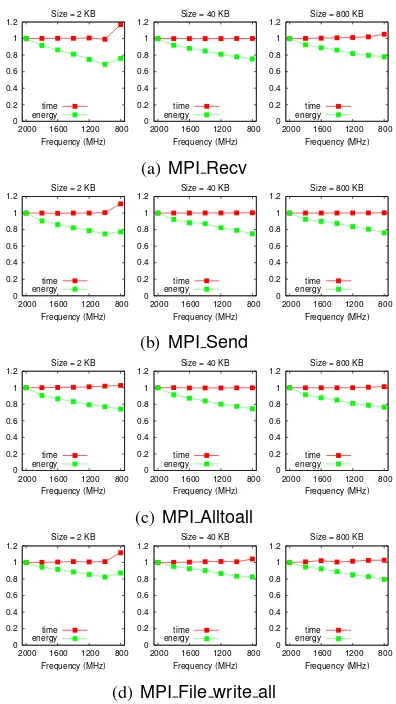
To be effective, reducing the p-state of the CPU should result in a large energy savings but a small time delay. As Figure 1 shows, MPI calls provide an excellent opportunity to reduce the p-state. Specifi-cally, this figure shows the time and energy as a func-tion of CPU frequency for four common MPI calls at several different sizes. (Function MPI File writeis included because it is used in BT and it communi-cates with a remote file system, which is a different action from other MPI communication calls.) For all MPI operations, at 1000 MHz at least 20% energy is saved with a time increase of at most 2.6%. The

0 0.2 0.4 0.6 0.8 1 1.2 800 1200 1600 2000 Frequency (MHz) Size = 2 KB

time energy 0 0.2 0.4 0.6 0.8 1 1.2 800 1200 1600 2000 Frequency (MHz) Size = 40 KB

time energy

(a)MPI Recv

time energy

(b)MPI Send

time energy

(c)MPI Alltoall

time energy

(d)MPI File write all

Figure 1: Micro-benchmarks showing time and en-ergy performance of MPI calls with CPU scaling.

greatest energy savings is 31% when receiving 2 KB at 1000 MHz. In addition, For the largest data size, the greatest time increase was only 5%. In terms of energy-delay product, the minimum is either 1000 or 800 MHz. Overall, these graphs show that MPI calls represent an opportunity, via CPU scaling, for energy saving with little time penalty.

(3)

0 0.1 0.2 0.3 0.4 0.5 0.6 0.7 0.8 0.9 1

0 5 10 15 20

Fraction of calls

Call length (ms) (a) CDF of MPI call length

0 0.2 0.4 0.6 0.8 1

0 10 20 30 40 50

Fraction of intervals

Time interval between MPI calls (ms) (b) CDF of inter MPI call interval

Figure 2: Cumulative distribution functions (CDF) of the duration of and interval between MPI calls for every MPI call for all nine programs in our benchmark suite.

will increase if one tries to save energy during such short MPI routines. Figure 2(b) plot the CDF for the interval between MPI calls. It shows that 96% of in-tervals are less than 5 milliseconds, which indicates that MPI calls clustered in time.

Hence, we need to amortize the cost of changing the p-state over several MPI calls. This brings up the problem of how to determine groups of MPI calls, or communication regions, that will execute in the same reduced p-state. The next section describes how we address this problem.

Finally, our solution only considers shifting at MPI operations. However, there are other places shifting can be done. For example, one could shift at program (computational) phase boundaries or even at arbitrary intervals. We rejected the latter because such shifting is not context-sensitive, meaning that we could not learn from previous iterations. The for-mer is context-sensitive, and with elaborate phase analysis it will likely find excellent shifting loca-tions. However, shifting only at MPI operations can easily be implemented transparently and in our tests was effective.

3 Design and Implementation

The overall aim of our system is to save significant energy with at most a small time delay. Broadly speaking, this research has three goals. First, it will identify program regions with a high concentration

of MPI calls. Second, it determines the “best” (re-duced) p-state to use during suchreducible regions. Both the first and second goals are accomplished with adaptivetraining. Third, it must satisfy the first two goals withno involvement by the MPI program-mer, i.e., finding regions as well as determining and shifting p-states should be transparent. In addition to the training component, the system has anshifting component. This component will effect the p-state shifts at region boundaries.

While we discuss the training and shifting com-ponents separately, it is important to understand that our system does not transition between these com-ponents. Instead, program monitoring is continuous, and training information is constantly updated. Thus our system is always shifting using the most recent information. Making these components continuous is necessary because we may encounter a given re-gion twice before a different rere-gion is encountered.

To achieve transparency—i.e., to implement the training and shifting components without any user code modifications—we use our MPI-jack tool. This tool exploits PMPI [25], the profiling layer of MPI. MPI-jack transparently intercepts (hijacks) any MPI call. A user can execute arbitrary code before and/or after an intercepted call using pre and post hooks. Our implementation uses the same pre and post hook for all MPI calls.

(4)

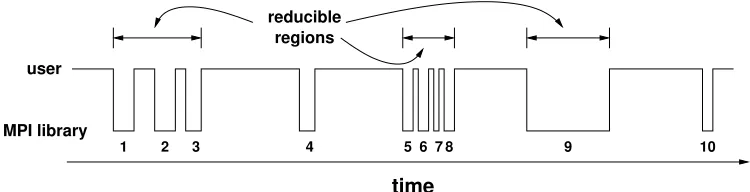
1 2 3 4 5 6 7 8 9 10

reducible regions user

time MPI library

Figure 3: This is an example trace of an MPI program. The line shows the type of code executed over time. There are 10 MPI calls, and calls 1–3 and 5–8 make up communication regions because they are close enough. Call 9 is con-sidered a region because it is long enough. Even though they are MPI calls, calls 4 and 10 are not in a communication region because they are neither close enough nor long enough.

is not a sufficient identifier. But it is easy to identify the dynamic parent of a call by examining the re-turn program counter in the current activation record. However, because an MPI call can be called from a general utility or wrapper procedure, one dynamic ancestor is not sufficient to distinguish the start or end of a region. Fortunately, it is simple and inex-pensive to examine all dynamic parents. We do this by hashing together all the return PCs from all acti-vation records on the stack. Thus, a call is uniquely identified by a hash of all its dynamic ancestors.

3.1 Assumptions

This work is based on two underlying assumptions. First, we assume that the CPU is not on the critical path during regions of communication, which also implies that it is beneficial to execute in a reduced p-state during this period. Our second assumption is that communication regions have a high concentra-tion of MPI calls. Therefore, we consider two MPI calls invoked in a short period of time to be part of the same communication region.

Figure 3 presents an example trace of an MPI pro-gram, where we focus solely on whether the program is in user code or MPI library code. The program be-gins in user code and invokes 10 MPI calls. In Fig-ure 3 there are two composite reducible regions—(1, 2, 3) and (5, 6, 7, 8). It also has a region consisting of only call 9 that is by itself long enough to be ex-ecuted in a reduce p-state. Thus, Figure 3 has three reducible regions, as well as two single MPI calls that will never execute in a reduce p-state.

3.2 The Training Component

The training component has two parts. The first is distinguishing regions. The second is determining the proper p-state for each region.

Starting from an MPI program withCcalls of MPI

routines, the goal is to group theCcalls intoR≤C

regions based on the distance in time between adja-cent calls, the time for a call itself, as well as the particular pattern of calls.

First, we must have some notion that MPI calls are close together in time. We denoteτ as the value

that determines whether two adjacent MPI calls are “close”—anything less than τ indicates they are.

Clearly, ifτ is ∞, then all calls are deemed to be

close together, whereas if it is zero, none are. Next, it is possible that an MPI call itself takes a signifi-cant amount of time, such as anMPI Alltoallusing a large array or a blockingMPI Receive. Therefore, we denoteλas the value that determines whether an

MPI call is “long enough”—any single MPI call that executes longer thanλwarrants reducing. Our tests

useτ = 10ms andλ= 10ms. Section 4.2 discusses

the rationale for these thresholds.

(5)

learned and updated as the program executes. For adaptive, there are many ways to learn. Next, we discuss two baseline region-finding algorithms, fol-lowed by two adaptive region-finding algorithms. Following that, we combine the best region-finding algorithm with automatic detection of the reduced p-state—this serves as the overall training algorithm that we have developed.

First, there is thebaseregion-finding algorithm, in which there are no regions—the program always ex-ecutes in the top p-state. It provides a baseline for comparison. Next, we denote by-callas the region-finding algorithm that treats every MPI call as its own region. It can be modeled asτ = 0 andλ = 0: no

calls are close enough and all are long enough. Sec-tion 2 explains thatby-callis not a goodgeneral so-lution because the short median length of MPI calls can cause the shifting overhead to dominate. How-ever, in some applications the by-call algorithm is very effective, saving energy without having to do any training.

We consider two adaptive region-finding algo-rithms. The first, called simple, predicts each call’s behavior based on what it did the last time it was encountered. For example, if a call ended a region last time, it is predicted to end a region the next time it appears. Thesimple method is effective for some benchmark programs. For example consider this pat-tern.

... AB... AB...AB...

Each letter indicates a particular MPI call invoked from the same call site in the user program; time proceeds from left to right. Variable τ is shown

graphically through the use of ellipses, which indi-cates that the calls are not close. The pattern shows that the distances betweenAandBare deemed close enough, but the gaps fromBtoAare not. Thus, the reducible regions in a program with the above pat-tern always begins withAand ends afterB. Because every Abegins a region and every Bends a region, once trained, thesimple mechanism accurately pre-dicts the reducible region every time thereafter.

However, there exist patterns for which simple is quite poor. Consider the following pattern.

... AA... AA...AA...

The gap between MPI calls alternates between less than and greater thanτ. However, in this caseboth

gaps are associated with thesame call. Because of this alternation, thesimplealgorithmalways mispre-dicts whetherAis in a reducible region—that is, in each groupsimplepredicts the firstAwill terminate a region because the secondAin the previous group did. The reverse happens when the second Ais en-countered. This is not a question of insufficient train-ing;simpleis not capable of distinguishing between the two positions thatAcan occupy.

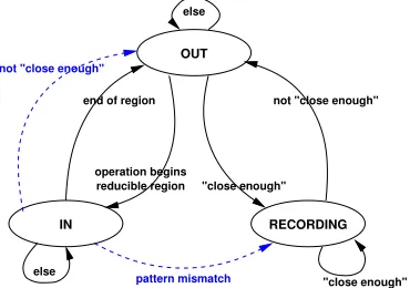
Our second region-finding algorithm, composite, addresses this problem. At the cost of a slightly longer training phase, composite collates informa-tion on aper-regionbasis. It then shifts the p-state based on what it learned the last time this region was encountered. It differs from simple in that it asso-ciates information with regions, not individual calls. Thecompositealgorithm matches the pattern of these calls and saves it; when encountered again, it will be able to determine that a region is terminated by the same final call.

The second part of training is determining the p-state in which to execute each region. As mentioned previously, extensive testing indicates that the MPI calls themselves can execute in very low p-states (1000 or 800 MHz) with almost no time penalty. However, a reducible region also contains user code between MPI calls. Consequently, we found that the “best” p-state is application dependent.

The overall adaptive training algorithm we advo-cate, calledautomatic, usescompositeto find regions and performance counters to dynamically determine the best p-state on a per-region basis. Specifically, in order to judge the dependence of the application on the CPU in these reducible regions, automatic measures the micro-operations1_{retired during the}

re-gion. It uses the rate micro-operations/microsecond (or OPS) as an indicator of CPU load. Thus a region with a low OPS value is shifted into a low p-state. Our system continually updates the OPS for each region via hardware performance counters. (This means the p-state selection for a region can change

1_{The AMD executes a RISC engine internally. It translates}

(6)

operation begins reducible region

IN

OUT

RECORDING "close enough"

pattern mismatch

not "close enough"

"close enough" else

else

end of region

not "close enough"

Figure 4: State diagram forcompositealgorithm.

over time.) Using large amounts of empirical test data, we developed by hand a single table that maps OPS to the desired p-state for a reduced region. This table is used for all benchmark programs, so it is not optimized for any particular benchmark.

3.3 The Shifting Component

There are two parts to the shifting component. The first is determining when a program enters and leaves a reducible region. The second part is effecting a p-state shift.

Thesimpleregion-finding algorithm maintains be-ginandendflags for each MPI call (or hash). The pre hook of all MPI calls checks the begin flag. If set, this call begins a region, so the p-state is reduced. Similarly, the post hook checks theendflag and con-ditionally resets the top p-state. This flag is updated every time the call is executed: it is set if the region was close enough or long enough and unset other-wise.

Figure 4 shows a state diagram for the compos-ite algorithm. There are three states: OUT,IN, and RECORDING. The processor executes in a reduced p-state only in the IN state; it always executes in the top p-state in OUT and RECORDING. The ini-tial state is OUT, meaning the program is not in a reducible region. At the beginning of a reducible re-gion, the system enters the IN state and shifts to a reduced p-state. The other state, RECORDING, is the training state. In this state, the system records a new region pattern.

The system transitions from OUT toIN when it encounters a call that was previously identified as

be-ginning a reducible region. If the call does not begin such a region but it was close enough to the previous call, the system transitions fromOUT to RECORD-ING. It begins recording the region from the previ-ous call. It continues recording while calls are close enough.

The system ordinarily transitions fromIN toOUT when it encounters the last call in the region. How-ever, there are two exceptional cases—shown with dashed lines in Figure 4. If the current call is no longer close enough, then the region is trun-cated and the state transitions to OUT. If the pat-tern has changed—this current call was not the ex-pected call—the system transitions toRECORDING. A new region is created by appending the current call to the prefix of the current region that has been ex-ecuted. None of the applications examined in Sec-tion 4 caused these excepSec-tional transiSec-tions.

Our implementation labels each region with the hash of the first MPI call in the region. When in the OUTstate at the beginning of each MPI call we look for a region with this hash as a label. If the region exists and is marked reducible, then we reduce the p-state and enter theINstate.

There are limitations to this approach if a single MPI call begins more than one region. The first prob-lem occurs when some of these regions are marked reducible and some are marked not reducible. Our implementation cannot disambiguate between these regions. The second problem occurs when one re-ducible region is a prefix of another. Because we do not know which region we are in (long or short), we cannot know whether to end the region after the prefix or not. A more sophisticated algorithm can be implemented that addresses both of these limita-tions; however, this was not done because it was not necessary for the applications examined. Rather, our system elects to be conservative in time, so our im-plementation executes in top p-state during all ambi-guities. However, this was not evaluated because no benchmark has such ambiguities.

(7)

MPI Reducible Calls Average time (ms) Time fraction

calls regions per region Per MPI Per region MPI region

EP 5 1 4 68.7 337.0 0.005 0.005

FT 46 45 1.0 18,400 18,810 0.849 0.860

IS 37 14 2.5 3100 8200 0.871 0.871

Aztec 20,767 301 68.9 2.04 143 0.806 0.812

CG 41,953 1977 21.2 6.90 149 0.753 0.768

MG 10,002 158 63.3 3.77 272 0.500 0.574

SP 19,671 8424 3.2 20.6 49.4 0.441 0.453

BT 108,706 797 136.7 8.39 1145 0.865 0.891

LU 81,874 766 107.2 1.11 356 0.149 0.446

Table 1: Benchmark attributes. Region information fromcompositewithτ = 10ms.

performed by the kernel. Thecpufreqandpowernow modules provide the basic support for this. Some additional tool support and significant “tweaking” of the FID-VID pairs was needed to refine the imple-mentation. The overhead of changing the p-state is dominated by the time to scale—not the overhead of the system call. For the processor used in these tests, the upper bound on a p-state transition (includ-ing system call overhead) is about 700 microseconds, but the average is less than 300 microseconds [12].

4 Results

This section presents our results in three parts. The first part discusses results on several benchmark pro-grams on a power-scalable cluster. These results were obtained by applying the different algorithms described in the previous section. The second part gives a detailed analysis of several aspects of our sys-tem and particular applications.

Benchmark attributes Eight of our benchmark

applications come from the NAS parallel benchmark suite, a popular high-performance computing mark [3]. The NAS suite consists of scientific bench-marks including application areas such as sorting, spectral transforms, and fluid dynamics. We test class C of these benchmarks. The benchmarks are unmodified with the exception of BT, which took far longer than all the other benchmarks; to reduce the time of BT without affecting the results, we exe-cuted it for 60 iterations instead of the original 200.

The ninth benchmark isAztecfrom the ASCI Purple benchmark suite [2].

Table 1 presents overall statistics of the bench-marks running on 8 or 9 nodes, which are distilled from traces that were collected using MPI-jack. The second column shows the number of MPI calls in-voked dynamically. The number of regions (column 3) is determined by executing the composite algo-rithm on the traces with the close enough threshold (τ) set to 10 ms. The table shows the average

num-ber of MPI calls per region in the fourth column. Be-cause some MPI calls are not in reducible regions, the product of the third and fourth columns is not necessarily equal to the second column. Next, the table shows the average time per MPI call and per reducible region. The last two columns show the fraction of the overall time spent in MPI calls and regions, respectively

The table clearly shows that these applications have diverse characteristics. In particular, in terms of the key region parameters—the number of regions, the number of calls per region, and the duration of the regions—there are at least two orders of magni-tude difference between the greatest and least values. Finally, with the exception of EP, the reducible frac-tion is at least 44%.

(8)

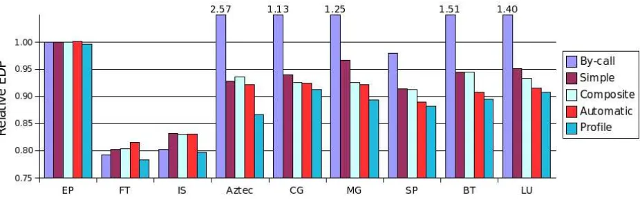
Figure 5: Overall EDP results for 5 methods relative to base case. For readability, the y-axis starts at 0.75.

algorithm.

Experimental methodology For all experiments,

we used a 10-node AMD Athlon-64 cluster con-nected by a 100Mbps network. Each node has 1 GB of main memory. The Athlon-64 CPU supports 7 p-states (from 2000 to 800 MHz). Each node runs the Fedora Core 3 OS and Linux kernel 2.6.8, and frequency shifting was done through thesysfs inter-face. All applications were compiled with eithergcc or the Intel Fortran compiler, using the O2 optimiza-tion flag. We controlled the entire cluster, so all ex-periments were run when the only other processes on the machines were daemons.

Elapsed time measurements are from the system clock using thegettimeofday system call. A power meter sits in between the system power supply of each node and the wall. We read this meter to get the power consumption. These readings are integrated over time to yield energy consumption. Thus the energy consumption measurements are empirically gathered for the system.

4.1 Overall Results

Our work trades time for energy. This tradeoff is difficult to evaluate because it has two dimensions, and users may assign different values to the trade-off. Energy-delay product (EDP) is one canonical evaluation metric. It is used here to convert the two-dimensional energy-time tradeoff into a single scalar metric. Figure 5 shows the EDP of each method rela-tive to the base case. This is a subset of the data in

Ta-ble 2. We conducted five tests for each of the bench-marks. For each test, the measured elapsed time and consumed energy are presented. EDP is computed from these empirical measurements. The value rela-tive to the base case is also presented. All tests were conducted a minimum of three times, with the me-dian value reported. The variance between any two runs was very small, so it is not reported.

As mentioned previously, the base test executes the program solely in top frequency (2000 MHz). Linux puts the processor into a low-power halt state when the run queue is empty, so we note that the base test is already power-efficient to some degree. Recall that the by-call, simple, and composite are purely region-finding algorithms and do not choose a particular p-state for regions. To provide a com-parison withautomatic, which uses OPS to choose the p-state on the fly, we did an exhaustive search of p-states. Then, the results forby-call,simple and compositereported in Figure 5 and Table 2 are those using the p-state yielding the lowest EDP.

(9)

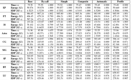
Base By-call Simple Composite Automatic Profile Time(s) 75.53 75.55 1.000 75.52 1.000 75.47 0.999 75.45 0.999 75.49 0.999

EP Energy(KJ) 59.876 59.878 1.000 59.857 1.000 59.878 1.000 59.946 1.001 59.669 0.997

EDP(MJ·s) 4.5225 4.5238 1.000 4.5202 1.000 4.5193 1.000 4.5289 1.001 4.5046 0.996

Time(s) 984.85 987.24 1.002 985.80 1.001 985.36 1.001 983.99 1.000 985.99 1.001

FT Energy(KJ) 606.45 479.24 0.790 486.21 1.802 487.41 0.804 494.91 0.816 475.13 0.783

EDP(MJ·s) 597.26 473.12 0.792 479.30 0.802 480.27 0.804 486.99 0.815 468.48 0.784

Time(s) 133.26 133.87 1.005 133.41 1.001 133.48 1.002 133.51 1.002 133.70 1.003

IS Energy(KJ) 79.102 63.236 0.799 65.768 0.831 65.465 0.828 65.604 0.829 62.891 0.795

EDP(MJ·s) 10.541 8.4655 0.803 8.7739 0.832 8.7379 0.829 8.7590 0.831 8.4086 0.798

Time(s) 51.94 85.98 1.655 55.80 1.074 55.55 1.069 53.55 1.031 53.86 1.037

Aztec Energy(KJ) 31.945 49.571 1.552 27.589 0.864 27.923 0.874 28.578 0.895 26.670 0.835

EDP(MJ·s) 1.6593 4.2619 2.568 1.5394 0.928 1.5510 0.935 1.5305 0.922 1.4364 0.866

Time(s) 378.50 414.87 1.096 402.81 1.064 396.74 1.048 393.49 1.039 396.14 1.047

CG Energy(KJ) 238.58 245.85 1.031 210.52 0.882 209.63 0.879 212.16 0.889 207.88 0.871

EDP(MJ·s) 90.301 101.00 1.130 84.801 0.939 83.565 0.925 83.484 0.924 82.348 0.912

Time(s) 76.84 90.35 1.176 81.90 1.066 78.87 1.027 78.67 1.024 78.88 1.027

MG Energy(KJ) 55.173 58.631 1.063 49.980 0.906 49.705 0.901 49.639 0.900 48.058 0.871

EDP(MJ·s) 4.2393 5.2971 1.250 4.0933 0.966 3.9204 0.925 3.9051 0.921 3.7909 0.894

Time(s) 910.85 944.86 1.037 938.16 1.030 938.38 1.030 945.40 1.038 932.00 1.023

SP Energy(KJ) 758.56 715.92 0.944 672.85 0.887 672.01 0.886 650.80 0.858 653.86 0.862

EDP(MJ·s) 690.94 676.44 0.979 631.24 0.914 630.60 0.913 615.27 0.890 609.42 0.882

Time(s) 1027.2 1295.5 1.261 1061.3 1.033 1057.1 1.029 1040.3 1.013 1029.3 1.002

BT Energy(KJ) 646.01 774.96 1.200 590.38 0.914 592.93 0.918 579.35 0.897 577.01 0.893

EDP(MJ·s) 663.58 1003.94 1.513 626.54 0.944 626.80 0.945 602.67 0.908 593.92 0.895

Time(s) 628.74 841.69 1.339 662.94 1.054 654.67 1.041 657.12 1.045 658.83 1.048

LU Energy(KJ) 489.08 510.24 1.043 441.24 0.902 438.14 0.896 428.24 0.876 423.19 0.865

EDP(MJ·s) 307.51 429.46 1.397 292.51 0.951 286.83 0.933 281.41 0.915 278.81 0.907 Table 2: Overall performance of benchmark programs. Where appropriate, the value relative to the base case is also reported. The p-state used insimpleandcompositeis the one found to have thebestenergy-delay product.

depending on the OPS.

The applications fall into several categories based on the performance of the algorithms. EP executes less than 0.5% of the total execution time in MPI calls, so no energy savings is possible with our mech-anisms. Thus we do not evaluate EP any further.

The second category contains FT and IS, appli-cations that perform well with the trivial by-call method. These are the only two applications that have singleton regions—an individual MPI call that is longer than λ, thus allowing a reduction in the

p-state. In FT, no calls are within τ. The average

length of MPI calls is 18.4 and 3.1 seconds for FT and IS, respectively. Consequently, the reducible re-gions are almost entirely MPI code and the reduced p-state is 800 MHz—the lowest p-state. As a result, these two benchmarks have the greatest energy sav-ing. Although these programs are in the reduced p-state more than 85% of the time, the increase in ex-ecution time is less than 1%. Therefore, the EDP is very low. This is our best case in terms of EDP, but most applications do not fall into this category. For example, SP is the only other benchmark that has an

energy savings using by-call because it has a rela-tively large average time per MPI call.

The next class of programs are ones for which by-callperforms poorly due to excessive p-state switch-ing, butsimpleis adequate. In our benchmark suite, this includes only Aztec. The pattern of MPI calls in Aztec is such thatsimple predicts well so there are few false positives forcomposite to remove. More-over, the longer training required bycomposite cre-ates false negatives—which are lost opportunities to save energy—that do not occur insimple. Therefore, compositeactually spends more time in the wrong p-state thansimple. As a result,simple is 0.7% lower in EDP, 1% less energy but 0.5% more time, than composite.

(10)

compos-ite and automatic. On the other hand, there is no difference between the region finding of simpleand composite in BT and SP. The automatic algorithm has a lower EDP than simple or compositebecause it is not limited to selecting a single reduced p-state. The improvement ofautomaticis due to the dynamic selection of a reduced p-state for each region. LU benefits from both improved region finding and mul-tiple p-state selection.

FT is the only application for which automaticis not as good as composite. The reason is that the region characteristics change over time. Accord-ing to OPS, the best gear for the primary region should be 1200 MHz for the first occurrence and 800 MHz thereafter. Thecomposite algorithm uses 800 MHz for all, automatic first uses 2000 MHz, then 1200 MHz, and not until the third occurrence does it select 800 MHz. This delay in determining the best p-state results in a 1.1% higher EDP in au-tomaticthan incomposite. Again, keep in mind that composite (and simple and by-call) is using the p-state that was best over all possibilities.

Finally, the rightmost column shows the perfor-mance of profile. In all cases, profile has the best EDP; this is expected because it uses prior applica-tion knowledge (a separate profiling execuapplica-tion). The usefulness ofprofileis that it serves as a rough lower bound on EDP. It is not a precise lower bound be-cause of several reasons, including that the reduced p-state in a given region cannot be proven to be best for EDP. However, generally speaking, if a given al-gorithm results in EDP that is close to profile, it is successful.

Summary In summary, simple is generally better

than by-calldue to less p-state switching overhead. However, composite is generally better than simple because it has, for several benchmarks, far fewer false positives at the cost of a a small number of ad-ditional false negatives. Finally, automatic is better thansimple orcomposite in all programs except for FT (IS is within experimental error), because using a customized p-state for each region is better than a single p-state—even the best one possible based on exhaustive testing—for the whole program.

4.2 Detailed Analysis

This section focuses on the details of how we achieved the performance reported in the previous section. In particular, it explains overhead then it discusses false negatives and positives. Finally, it in-vestigates how we selected our threshold values.

System Overhead This paragraph discusses the

overhead of the system in two parts. The first part is the overhead of changing p-states. As stated above on this AMD-64 microprocessor the average cost to shift between p-states is slightly less than 300 mi-croseconds. The greatest time to shift is just un-der 700 microseconds [12]. The actual cost of this overhead depends on the number of shifts between p-states, which is twice the number of reducible gions. Table 1 shows that the shortest average re-gion length is approximately 50 milliseconds, which is more than 160 times longer than the average shift cost. Thus the overhead due to shifting is nominal.

The second part of the overhead is due to data col-lection, which happens at the beginning and end of each MPI call. The overhead consists of three parts: hijacking the call, reading system time, and reading the performance counters. The first two parts occur every MPI call, while the latter occurs only at the be-ginning and end of each region. The cost of all three parts is approximately 1.3 microseconds. Because shifting p-states changes elapsed time, we cannot di-rectly compare the overhead of our technique to the baseline, which does not shift. To measure the over-head of the algorithm only, we modified the system to perform all steps except shifting. In this case, we can compare elapsed time to the baseline. The rela-tive cost of this overhead is less than 1% on all the NAS programs (the greatest overhead is 0.38% for LU).

False negatives and positives Figure 6 compares

(11)

(a)simple

(b)composite

Figure 6: Breakdown of execution time for adaptive region-finding algorithms.

shows thepotentialimpact by showing how much of the base code is effected by our scaling.

This analysis divides the base, unscaled time into into four categories along two dimensions: (a)INor OUT of a reducible region and (b)trueorfalse pre-diction. Correct predictions are determined by ex-amining trace data, as is done inprofile. In Figure 6, bars labeled “IN (true)” and “OUT (true)” are cor-rectly predicted. The bar labeled “IN (false)” is a false positive; the application mistakenly executes in a reduced p-state instead of the top p-state. The bar labeled “OUT (false)” is a false negative; the appli-cation mistakenly executes in the top p-state instead of a reduce one. Generally, a false positive is consid-ered worse than a false negative because it can result in a time penalty. In contrast, a false negative repre-sents an energy saving opportunity lost.

For FT and IS,simple has false negatives, which explains why it is worse in EDP thanby-call. Thus, simple is slightly faster but consumes more energy. Furthermore, with singleton regions there is no

dif-ference in the predictive power ofsimple and com-posite. These plots show that the longer training period in composite adds false negatives to Aztec and BT. But because neither application has signifi-cant false positives to eliminate,simpleperforms bet-ter than composite. For the remaining three bench-marks, composite eliminates significant mispredic-tions compared tosimple. For CG and LU there are in fact no mispredictions incomposite. For MG, all false positive cases are eliminated as well.

Choosingτ Figure 7 shows data for evaluatingτ,

the threshold that determines whether two MPI rou-tines are “close enough.” This evaluation is done withcomposite. Three metrics are plotted: the frac-tion of time for false negatives, the fracfrac-tion of time for false positives, and the number of regions.

Clearly, there is a tension in the choice ofτ. Ifτis

too large, then a few, large regions will result. This means that when using automatic, a large number of false negatives would result, which in turn would result in a significant fraction of time due to them. For example, ifτ =∞, the training component will

run the whole program, and the executing component will never run—the entire program is a false nega-tive. On the other hand, ifτ is too small, then

auto-maticwould approachby-call, which we know from Section 4.1 is often an ineffective algorithm due to excessive time due to p-state shifting.

Indeed, the figure shows that the value ofτ has a

significant impact on benchmarks that have several short MPI calls (EP, IS, and FT do not and so are not in the figure). The goal is, essentially, to choose forτ the smallest value possible such that the region

overhead (which is proportional to the number of re-gions) is small. While there is not a choice that works for all benchmarks—for CG it is around 45 ms, for BT 48 ms, but for the others, it is closer to 10 or 20 ms. The one problematic application is SP, which has numerous short regions, and the choice of a longerτ

can reduce EDP by more than 2%. We are currently addressing this issue.

Choosing λ The duration of MPI calls over all

(12)

0 0.2 0.4 0.6 0.8 1

0 20 40 60 80 100 0 500 1000 1500 2000

Fraction of time _{Number of regions}

τ (ms) False neg

False pos Regions (a) CG 0 0.2 0.4 0.6 0.8 1

0 20 40 60 80 100 0 200 400 600 800 1000

τ (ms) False neg

False pos Regions (b) BT 0 0.2 0.4 0.6 0.8 1

0 20 40 60 80 100 0 200 400 600 800 1000

τ (ms) False neg

False pos Regions (c) LU 0 0.2 0.4 0.6 0.8 1

0 20 40 60 80 100 0 200 400 600 800 1000

τ (ms) False neg

False pos Regions (d) MG 0 0.2 0.4 0.6 0.8 1

0 20 40 60 80 100 0 2000 4000 6000 8000 10000

τ (ms) False neg

False pos Regions (e) SP 0 0.2 0.4 0.6 0.8 1

0 20 40 60 80 100 0 200 400 600 800 1000

τ (ms) False neg

False pos Regions (f) Aztec

Figure 7: Evaluatingτ incomposite. Show fraction of time mispredicted and number of regions (right-hand

y-axis) as a function ofτ. For readability, right-hand y-axis has different scale for CG and SP.

MPI calls over the programs, because the calls in IS and FT take 3 and 18 seconds, respectively. Thus all values ofλbetween 10 and 2000 ms achieve the

same result. We do point out, though, that for differ-ent benchmarks, where the calls may be more evenly distributed, much more thought would need to go into choosingλ.

5 Related Work

The most relevant related work to this paper is in high-performance, power-aware computing. Several researchers have addressed saving energy with min-imal performance degradation. Cameron et al. [5] uses a variety of different DVS scheduling strate-gies (for example, both with and without application-specific knowledge) to save energy without signifi-cantly increasing execution time. A similar run-time effort is due to Hsu and Feng [18]. Our own prior work is fourfold: an evaluation-based study that fo-cused on exploring the energy/time tradeoff in the NAS suite [14], development of an algorithm for switching p-states dynamically between phases [13], leveraging load imbalance to save energy [21], and minimizing execution time subject to a cluster

en-ergy constraint [28].

The difference between all of the above research and this paper is the type of bottleneck we are at-tacking. This is the first work we know of to address the communication bottleneck.

The above approaches strive to save energy for a broad class of scientific applications. Another ap-proach is to save energy in an application-specific way; the work in [8] used this approach for a parallel sparse matrix application.

(13)

Additional approaches have been taken to include dynamic voltage scaling (DVS) and request batch-ing [10]. The work in [26] applies real-time tech-niques to web servers in order to conserve energy while maintaining quality of service.

In server farms, disk energy consumption is also significant; several have studied reducing disk en-ergy (e.g., [6, 30, 23]). In this paper, we do not consider disk energy as it is generally less than CPU energy, especially if scientific programs operate pri-marily in core.

Our work attempts to infer regions based on rec-ognizing repeated execution. Others have had the same goal and carried it out using the program counter. Gniady and Hu used this technique to de-termine when to power down disks [16], along with buffer caching pattern classification [15] and ker-nel prefetching [4]. In addition, dynamic techniques have been used to find program phases [20, 9, 27], which is tangentially related to our work.

6 Conclusion

This paper has presented a transparent, adaptive system for reducing the p-state in communication phases. The basic idea is to find such regions on the fly by monitoring MPI calls and keep a state machine that recognizes the regions. Then, we use performance counters to guide our system to choose the best p-state in terms of energy-delay product (EDP). User programs can use our runtime system with zero user involvement. Results on the NAS benchmark suite showed an average 10% reduction in EDP across the NAS suite.

Our future plans include integrating the idea of reducing the p-state during communication regions with our past work on reducing the p-state during computation regions. Additionally, we will conduct these experiments on a newer cluster, which has a gi-gabit network and multi-core, multiprocessor nodes. For computation, we leverage the memory or node bottleneck to save energy, sometimes with no in-crease in execution time. The overall goal is to de-sign and implement one MPI runtime system that si-multaneously exploits all three bottlenecks.

References

[1] N.D. Adiga et al. An overview of the BlueGene/L supercomputer. In Supercomputing, November 2002.

[2] ASCI Purple Benchmark Suite. http://www.llnl.-gov/asci/platforms/purple/rfp/benchmarks/. [3] D. Bailey, J. Barton, T. Lasinski, and H. Simon.

The NAS parallel benchmarks. RNR-91-002, NASA Ames Research Center, August 1991.

[4] Ali Raza Butt, Chris Gniady, and Y. Charlie Hu. The performance impact of kernel prefetching on buffer cache replacement algorithms. In SIGMETRICS, pages 157–168, 2005.

[5] K.W. Cameron, X. Feng, and R. Ge. Performance-constrained, distributed dvs scheduling for scientific applications on power-aware clusters. In Supercom-puting, November 2005.

[6] Enrique V. Carrera, Eduardo Pinheiro, and Ricardo Bianchini. Conserving disk energy in network servers. In Intl. Conference on Supercomputing, June 2003.

[7] Jeffrey S. Chase, Darrell C. Anderson, Prachi N. Thakar, Amin Vahdat, and Ronald P. Doyle. Man-aging energy and server resources in hosting cen-tres. InSymposium on Operating Systems Princi-ples, 2001.

[8] Guilin Chen, Konrad Malkowski, Mahmut Kan-demir, and Padma Raghavan. Reducing power with performance contraints for parallel sparse applica-tions. InWorkshop on High-Performance, Power-Aware Computing, April 2005.

[9] A. Dhodapkar and J. Smith. Comparing phase de-tection techniques. InInternational Symposium on Microarchitecture, pages 217–227, December 2003. [10] Elmootazbellah Elnozahy, Michael Kistler, and Ra-makrishnan Rajamony. Energy conservation poli-cies for web servers. InUsenix Symposium on Inter-net Technologies and Systems, 2003.

[11] E.N. (Mootaz) Elnozahy, Michael Kistler, and Ra-makrishnan Rajamony. Energy-efficient server clus-ters. InWorkshop on Mobile Computing Systems and Applications, Feb 2002.

(14)

[13] Vincent W. Freeh, David K. Lowenthal, Feng Pan, and Nandani Kappiah. Using multiple energy gears in MPI programs on a power-scalable cluster. In Principles and Practices of Parallel Programming, June 2005.

[14] Vincent W. Freeh, David K. Lowenthal, Rob Springer, Feng Pan, and Nandani Kappiah. Explor-ing the energy-time tradeoff in MPI programs on a power-scalable cluster. InInternational Parallel and Distributed Processing Symposium, April 2005. [15] Chris Gniady, Ali Raza Butt, and Y. Charlie

Hu. Program-counter-based pattern classification in buffer caching. InOSDI, pages 395–408, 2004. [16] Chris Gniady, Y. Charlie Hu, and Yung-Hsiang

Lu. Program counter based techniques for dynamic power management. InHPCA, pages 24–35, 2004. [17] Richard Goering. Current physical design tools

come up short. EE Times, April 14 2000.

[18] Chung hsing Hsu and Wu chun Feng. A power-aware run-time system for high-performance com-puting. InSupercomputing, November 2005. [19] Chung-Hsing Hsu and Wu-chun Feng. Effective

dynamic-voltage scaling through CPU-boundedness detection. In Fourth IEEE/ACM Workshop on Power-Aware Computing Systems, December 2004. [20] M. Huang, J. Renau, and J. Torellas. Positional

adaptation of processors: Application to energy re-duction. InInternational Symposium on Computer Architecture, June 2003.

[21] Nandani Kappiah, Vincent W. Freeh, and David K. Lowenthal. Just in time dynamic voltage scaling: Exploiting inter-node slack to save energy in MPI programs. InSupercomputing, November 2005. [22] Charles Lefurgy, Karthick Rajamani, Freeman

Raw-son, Wes Felter, Michael Kistler, and Tom W. Keller. Energy management for commerical servers. IEEE Computer, pages 39–48, December 2003.

[23] Athanasios E. Papathanasiou and Michael L. Scott. Energy efficiency through burstiness. InWorkshop on Mobile Computing Systems and Applications, October 2003.

[24] Eduardo Pinheiro, Ricardo Bianchini, Enrique V. Carrera, and Taliver Heath. Load balancing and unbalancing for power and performance in cluster-based systems. InWorkshop on Compilers and Op-erating Systems for Low Power, September 2001.

[25] Rolf Rabenseifner. Automatic profiling of MPI ap-plications with hardware performance counters. In PVM/MPI, pages 35–42, 1999.

[26] Vivek Sharma, Arun Thomas, Tarek Abdelzaher, and Kevin Skadron. Power-aware QoS management in web servers. InIEEE Real-Time Systems Sympo-sium, Cancun, Mexico, December 2003.

[27] Timothy Sherwood, Erez Perelman, Greg Hamerly, and Brad Calder. Automatically characterizing large scale program behavior. InArchitectural Support for Programming Languages and Operating Systems, October 2002.

[28] Robert C. Springer IV, David K. Lowenthal, Barry Rountree, and Vincent W. Freeh. Minimizing execution time in MPI programs on an energy-constrained, power-scalable cluster. InACM Sym-posium on Principles and Practice of Parallel Pro-gramming, March 2006.

[29] M. Warren, E. Weigle, and W. Feng. High-density computing: A 240-node beowulf in one cubic meter. InSupercomputing, November 2002.