SLANTLET TRANSFORM-BASED SEGMENTATION AND α -SHAPE THEORY-BASED 3D VISUALIZATION AND VOLUME CALCULATION
METHODS FOR MRI BRAIN TUMOUR
MOHAMMED SABBIH HAMOUD AL-TAMIMI
A thesis submitted in fulfilment of the requirements for the award of the degree of
Doctor of Philosophy (Computer Science)
Faculty of Computing Universiti Teknologi Malaysia
I would like to dedicate this work for
my beloved wife "Hala" and lovely kids
"Malak & Hussein"
ACKNOWLEDGEMENT
Thanks to Allah SWT for everything I was able to achieve and for everything I tried, but I was not able to achieve.
To my supervisor Professor Dr. Ghazali Bin Sulong, you are truly a SUPER-visor. I am greatly appreciative of him for his support and guidance, most importantly, for providing me the freedom to pursue my ideas and find my own path in research. Also, I have gained a wealth of experience and knowledge working under your supervision, which will always be my delight to share along my life’s journey. Thanks also to Consultant Radiologists, Professor Dr. Ibrahim Shuaib, and Dr. Zahari Mahbar for their involvement in this research.
To my beloved father, Professor Dr. Sabbih H. Al-Tamimi, thank you for bringing a side of me. I will always cherish your limitless support and encouragement.
ABSTRACT
ABSTRAK
TABLE OF CONTENTS
CHAPTER TITLE PAGE
DECLARATION ii
DEDICATION iii
ACKNOWLEDGEMENT iv
ABSTRACT v
ABSTRAK vi
TABLE OF CONTENTS vii
LIST OF TABLES xiii
LIST OF FIGURES xvi
LIST OF ABBREVIATIONS xxxi
LIST OF SYMBOLS xxxiv
LIST OF ALGORITHMS xxxvi
LIST OF APPENDICES xxxviii
1 INTRODUCTION 1
1.1 Overview 1
1.2 Designations 3
1.3 Background of Research 6
1.4 Problem Statements 13
1.5 Research Goal 15
1.6 Objectives of the Study 15
1.7 Research Scope 15
1.8 Significance of the Study 16
2 LITERATURE REVIEW 19
2.1 Introduction 19
2.2 Medical Glossary of Brain Tumour 20
2.2.1 Brain Anatomy 21
2.2.2 Brain Tumour 23
2.2.3 MRI Brain Imaging 24
2.3 Detetection Abnormal Slices in Magnetic
Resonance Images 25
2.3.1 Cerebral Tissues Extraction 26 2.3.1.1 Cerebral Tissues Extraction
Based on Intensity 28
2.3.1.2 Cerebral Tissues Extraction
Based on Morphology 29
2.3.1.3 Cerebral Tissues Extraction
Based on Deformation 30
2.3.2 Classification Methods for Detecting
Abnormality in Brain MR Images 32
2.4 Medical Image Segmentation 34
2.4.1 Spatial Clustering 36
2.4.2 Split and Merge Segmentation 36
2.4.3 Region Growing 37
2.4.4 Computational Techniques for Medical
Image Segmentation 37
2.4.4.1 Thresholding Based Methods 38 2.4.4.2 Region Growing Based
Methods 40
2.4.4.3 Neural Networks Based
Methods 43
2.4.4.4 Fuzzy Based Methods 45
2.4.4.5 Hybrid Techniques 49
2.4.4.6 Other Brain Tumour
Techniques
2.5 Volumetric Calculation and 3D Visualization of
Brain Tumour in MRI 57
2.6 Alpha (α) Shape Theory 59
2.6.1 Modelling and Visualization Using
α-Shape Theory 62
2.6.2 Limitations of α-Shape 63
2.6.3 Determination of the Best α Value 65 2.6.3.1 Small α Values Selection 65 2.6.3.2 Large α Values Selection 67 2.6.3.3 Selecting α Value “Just Right” 67
2.7 Summary 68
3 A CONCEPTUAL FRAMEWORK 70
3.1 Introduction 70
3.2 Research Framework 71
3.3 Operational Research Framework 74
3.4 Validation of the Proposed Methods 77
3.4.1 Quantitative Evaluation 78
3.4.1.1 Jaccard and Dice Coefficients 79 3.4.1.2 Sensitivity, Specificity and
Accuracy 80
3.4.2 Qualitative Evaluation 81
3.5 Benchmarking 82
3.5.1 Frustum Model 83
3.5.2 Meshing Point Clouds 83
3.5.3 Trace Method 83
3.5.4 Modified MacDonald (MMC) Method 84
3.6 Dataset 85
3.6.1 IBSR (10Normals_T1) Dataset 87
3.6.2 IBSR (536_T1) Dataset 89
3.6.3 Challenge MICCAI
3.7 Creation of Two Ground Truth 95
3.8 Summary 105
4 DESIGN AND IMPLEMENTATION OF
PROPOSED METHOD 107
4.1 Introduction 107
4.2 Detection of Abnormal MRI Slices 108
4.2.1 Extraction of the Cerebral Tissues 109
4.2.1.1 Image Binarization 111
4.2.1.2 Largest Connected
Component 113
4.2.1.3 Masking 118
4.2.1.4 Bitwise Operation “AND” 119 4.2.2 Determination of Thresholds 121 4.2.2.1 Features Extraction 124 4.2.2.2 Mean, Energy and Entropy
Distribution 126
4.2.2.3 Mean, Energy and Entropy
Correlation 131
4.2.3 Detection of Abnormal Blocks 134 4.3.2.1 Fine-tuning of Abnormal
Blocks 135
4.3 Automatic Segmentation of Brain Tumour Based
on Slantlet Transform 142
4.3.1 Slantlet Transform Decomposition 143 4.3.2 Selection of Significant SLT
Coefficients 154
4.3.3 Inverse Slantlet 157
4.4 3D Visualization and Volumetric Measurement
Using α-Shapes Theory
4.4.3.1 Construction of α-Shapes 166 4.4.3.2 Delaunay Triangulation 167 4.4.3.3 Implementation of Delaunay
Triangulation 170
4.4.3.4 α-Shapes Implementation 178 4.4.4 Brain Tumour 3D Visualization and
Volume Calculation 182
4.5 Summary 183
5 QUALITATIVE AND QUANTITATIVE
EXPERIMENTAL RESULT 184
5.1 Introduction 184
5.2 Result of Abnormal Slice Detection 186 5.2.1 Results of Cerebral Tissue Extraction 186 5.2.2 Results of the Abnormal Block
Detection Before the Fine-tuning 190 5.2.3 Results of the Fine-tuning of Abnormal
Block detection 197
5.2.4 The Quantitative Assessment of the
Tumour Block Detection 207
5.2.4.1 Quantitative Evaluation of
Slice Abnormality Detection 215 5.3 Performance Evaluation of the Proposed
SLT-based Segmentation Technique 221
5.3.1 Results and Discussions of the
Qualitative Evaluation 222
5.3.2 Results and Discussions of the
Quantitative Evaluation 228
5.4 Performance Evaluation of 3D Visualization and
Volume Calculation of Brain Tumours 235 5.4.1 Qualitative Evaluation of 3D
5.4.2 Quantitative Evaluation of Brain
Tumour Volume Calculation 250
5.5 Summary 256
6 CONCLUSIONS AND FURTHER OUTLOOK 258
6.1 Contributions 261
6.2 Further Outlook 263
REFERENCES 265
LIST OF TABLES
TABLE NO. TITLE PAGE
2.1 Relevant literatures on thresholding based methods 39 2.2 Relevant literatures on region growing based
methods 41
2.3 Relevant literatures on NN based methods 45
2.4 Relevant literatures on Fuzzy based methods 47 2.5 Relevant literatures on Hybrid techniques 50 2.6 Relevant literatures on other brain tumour
segmentation and detection techniques 53 3.1 Summary of the operational research framework 75
3.2 Validation of the proposed methods 77
3.3 Definition of TP, TN, FN, and FP 80
3.4 Existing methods for benchmarking of different
processes 82
3.5 Properties of normal patient from IBSR
(10Normals_T1) dataset 89
3.6 Properties of abnormal patient from IBSR (536_T1)
dataset 92
3.7 Properties of challenge MICCAI
(BRATS2012-BRATS-1) dataset 95
3.8 Hitachi Airs MRI device specifications 98
3.9 The computer specifications of Hitachi Airs MRI
device 99
3.11 Calculation of displaced water weight of the six
irregular objects 104
3.12 The ground truth volume of all irregular objects
(solid and hollow) 105
4.1 The pixel count of each region in MRI slice “I” 116 4.2 The threshold values of mean, energy and entropy
for the different datasets 134
4.3 ROI dimension according to SLT filter-bank 149 4.4 The values of slice thickness and pixel spacing of
MR images from different sources 163
5.1 Block abnormality detection results of the IBSR
(10Normals_T1) dataset 208
5.2 Block abnormality detection results of the IBSR
(536_T1) dataset 211
5.3 Block abnormality detection results of the challenge
MICCAI (BRATS2012-BRATS-1) dataset 213
5.4 Experimental results of slice abnormality detection
of IBSR (10Normals_T1) dataset 216
5.5 Experimental results of abnormality detection by
slice obtained from the IBSR (536_T1) dataset. 217 5.6 Experimental results of abnormality detection by
slice obtained from the challenge MICCAI
(BRATS2012-BRATS-1) dataset 218
5.7 Jaccard and Dice indices of the proposed method
implemented on the IBSR (536_T1) dataset 228 5.8 Jaccard and Dice indices of the proposed method
implemented on the challenge MICCAI
(BRATS2012-BRATS-1) dataset 229
5.9 Sensitivity, specificity, and accuracy of the proposed segmentation method implemented on
IBSR (536_T1) dataset 230
5.10 Sensitivity, specificity, and accuracy of the proposed segmentation method implemented on
5.11 Performance results of the proposed method versus the state-of-the-art techniques for the challenge
MICCAI (BRATS2012-BRAT-1) dataset 233
5.12 Calculated volume of the six objects 251
5.13 The proposed method versus four standard volume measures in terms volume error rates of six
irregular objects 252
5.14 Calculated tumour volumes of IBSR (536_T1) dataset: Comparison between the proposed method
and the four standard measures 254
5.15 Calculated tumour volumes of challenge MICCAI (BRATS2012-BRATS-1) dataset: Comparison between the proposed method and the four standard
LIST OF FIGURES
FIGURE NO TITLE PAGE
1.1 Human brain slices with different imaging modalities. From left to right: CT, MRI, SPECT
and PET (Wright 2010) 4
1.2 MR brain image from patient’s head (a) The setup, (b) Axial plane view, (c) Sagittal plane view, and
(d) Coronal plane view (Lorenzen et al. 2001) 5 1.3 MR image sequence (Brown and Semelka 2011) 6 1.4 Normal MRI slices from IBSR (10Normals_T1)
dataset, (a) Slice 22 of patient Normal_4, and (b)
Slice 16 of patient Normal_15 7
1.5 Normal MRI slices from challenge MICCAI (BRATS2012-BRATS-1) dataset, (a) Slice 119 of patient BRATS_HG0010, and (b) Slice 54 of
patient BRATS_HG0008 8
1.6 Abnormal MRI slices at different locations with varying size, shapes, and image intensities of brain tumour (red rectangle) from IBSR (536_T1) dataset of MRI scan 536_32, (a) Slice 22, and (b)
Slice 26 8
BRATS_HG0004, and (b) Slice 127 of patient
BRATS_HG0007 9
1.8 3D brain tumour visualization of MRI scan 536_32 in IBSR (536_T1) dataset using Matlab's Meshing
Point Clouds function 10
2.1 GM and WM brain tissues (Nolte 2013) 21
2.2 Normal circulation of CSF in the brain (Nolte
2013) 22
2.3 Major subdivision of human brain (Nolte 2013) 22 2.4 The working principle of MRI machine (Dominik
et al. 2008) 25
2.5 Slice 44 of MRI scan 536_88 in IBSR (536_T1) dataset, (a) with non-cerebral tissues, and (b)
without non-cerebral tissues 27
2.6 Typical results of cerebral tissues extraction, (a) Original MR image, (b) WAT extracted image
(Sadananthan et al. 2010) 28
2.7 Typical results of BSE cerebral tissues extraction, (a) Original MR image, (b) BSE extracted image
(Sadananthan et al. 2010) 29
2.8 Typical results of BET cerebral tissues extraction, (a)
Original MR image, (b) BET extracted image 31
2.9 Typical results of HWA cerebral tissues extraction, (a) Original MR image, (b) HWA extracted image
(Sadananthan et al. 2010) 31
2.10 (a) original image, (b) ground truth-based border image, (c) seeded image; (d) and (e) are segmentation results using the RGB a colour space presenting their best index; (f) and (g) are segmentation results using the adaptive discrimination function generated by the seed points presented in (c) with best rand index
2.11 Same set of points with: a) linear frontier, b)
convex hull, c) concave hull, and d) α-Shape 61 2.12 Examples of 3D model to form mesh of triangular
faces using α-shape theory 62
2.13 The interstice problem, (a) Break in the object surface, (b) Wrong interstice close using α-shape,
and (c) Right interstice close 63
2.14 Demonstration of the failure between surfaces at joints and interstices (a) Two separate objects, and (b) Wrong joint using α-shape, and (c) Right joint
close 64
2.15 α-shape with different values: (a) α = 0, (b) α =
0.19, (c) α = 0.25, (d) α = 0.75, (e) α = ∞ 64 2.16 A set of points representing the locations of bus
stations in a town 65
2.17 The α-shape created from the bus stations using α =
0.5 KM 66
2.18 The α-shape created from the bus stations using α =
3 KM 67
2.19 The α-shape created from the bus stations using α =
1.1 KM 68
3.1 An overview of the proposed methodology 72
3.2 The detection / segmentation in MRI slices using
Jaccard and Dice coefficients 79
3.3 Two longest orthogonal diameters of the largest tumours for MRI scan 536_88 in IBSR (536_T1) dataset, (a) Original slice 28, (b) Tumour segmentation, (c) diameter d1 (blue line), and (d)
diameter d2 (green line) 85
3.4 Three MRI datasets used in the present research 86 3.5 3D views of 56 MRI slice of the patient Normal_8
living brain obtained from IBSR (10Normals_T1)
3.6 3D views of sixty MRI slices of the MRI scan 536_32 living brain obtained from IBSR (536_T1)
dataset 90
3.7 The ground truth of 3D views for sixty MRI slices of the MRI scan 536_32 living brain obtained from
IBSR (536_T1) dataset 91
3.8 3D views of 176 MRI slice of the patient’s living brain obtained from challenge MICCAI
(BRATS2012-BRATS-1) dataset 93
3.9 The ground truth of 3D views of 176 MRI slice of the patient’s living brain obtained from challenge
MICCAI (BRATS2012-BRATS-1) dataset 94
3.10 Four irregular solid objects (a) Meat, (b) Carrot, (c)
Egg, and (d) Cucumber 96
3.11 Irregular object with cavity, (a) Potato, and (b)
Green Pepper 96
3.12 The MRI scan process of six irregular objects 97
3.13 2006 Hitachi Airis Elite 0.3T Open MRI 97
3.14 The MRI scan of an egg, (a) MR slices images, and
(b) MR slices with segmented egg images 99 3.15 The MRI scan of a potato, (a) MR slices of egg
images, and (b) MR slices with segmented potato
images 100
3.16 Mettler AT400 balance 101
3.17 The mass calculation of (a) Green Pepper, (b) Potato, (c) Cucumber, (d) Egg, (e) Carrot, and (f)
Meat 102
3.18 Beaker glass of volume (a) 1000 ml, and (b) 250
ml 103
3.19 Water displacement calculations, (a) Green pepper, (b) Egg, (c) Potato, (d) Carrot, (e) Meat, and (f)
Cucumber 104
4.1 Flowchart of the proposed method for the detection
4.2 The proposed method for extraction cerebral
tissues from MRI slices 111
4.3 A sample of binary MRI slice 114
4.4 Four detected regions (1 to 4) of a binary MRI slice 115
4.5 The largest region or the detected LCC 116
4.6 Detected LCC in MRI scan 536_32 of IBSR (536_T1) dataset, (a) Slice 14, (b) Slice 37, (c)
Slice 45, and (d) Slice 52 117
4.7 The connected components of MRI scan 536_32 in IBSR (536_T1) data set, (a) Original slice 9, and (b) Three different connected components (red,
green, and blue) 120
4.8 The cerebral tissue extraction of MRI scan 536_32 in IBSR (536_T1) dataset, (a) Original slice 9, (b) Binary image with three connected components (white regions), (c), the LCC (the largest white region), (d) the LCC mask (black region), and (e)
Extracted cerebral tissue 120
4.9 The probability of the tumour occurrence in MR
image slices for IBSR (536_T1) dataset 122 4.10 Tumour occurrence probability in MR image slices
for challenge MICCAI (BRATS2012-BRATS-1)
dataset 123
4.11 Non-overlapping block partition of patient Normal_19 of IBSR (10Normals_T1) dataset, (a) Original slice 23, and (b) Non-overlapping block
division using (8×8) block size 124
4.12 Non-overlapping block partition of patient BRATS_HG0009 of challenge MICCAI (BRATS2012-BRATS-1) dataset, (a) Original slice 103, and (b) Non-overlapping block division using
(8×8) block size 125
patient BRATS_HG0015 of challenge MICCAI (BRATS2012-BRATS-1) dataset using (8×8) block size
4.14 Manual identification of slice 88 for patient BRATS_HG0015 of challenge MICCAI (BRATS2012-BRATS-1) dataset into Normal (N)
and Abnormal (A) regions 128
4.15 Distribution of mean of slice 88 for patient BRATS_HG0015 of challenge MICCAI
(BRTAS2012-BRATS-1) dataset 129
4.16 Distribution of entropy of slice 88 for patient BRATS_HG0015 of challenge MICCAI
(BRTAS2012-BRATS-1) dataset 129
4.17 Distribution of energy of slice 88 for patient BRATS_HG0015 of challenge MICCAI
(BRTAS2012-BRATS-1) dataset 130
4.18 Relation among mean, energy, and entropy of slice 88 for patient BRATS_HG0015 of challenge
MICCAI (BRTAS2012-BRATS-1) dataset 131 4.19 The relationship between mean and energy of slice
88 for patient BRATS_HG0015 in challenge
MICCAI (BRTAS2012-BRATS-1) dataset 132
4.20 The relationship between entropy and energy of slice 88 for patient BRATS_HG0015 in challenge
MICCAI (BRTAS2012-BRATS-1) dataset 132
4.21 The relationship between entropy and mean of slice 88 for patient BRATS_HG0015 in challenge
MICCAI (BRTAS2012-BRATS-1) dataset 133
4.22 Abnormal block detections rules 134
4.23 Three types of block masks with size (3×3) called preceding mask centred at Pi, current mask centred at Ci, and succeeding mask centred at Si. Green
colour indicates ignored block 136
patient BRATS_HG0011 in challenge MICCAI (BRATS2012-BRATS-1) dataset
4.25 Fine-tuning of Case 1: (a1) → (a2), and Case 2:
(b1) → (b2), where the mechanism changes the
block Ci based on its neighbours 137
4.26 Fine-tuning of (Case 3 - Case 6), where Ci is changed from tumour to a non-tumour block using
the Rule 1 138
4.27 Fine-tuning of (Case 7 - Case 10), where Ci is changed from non-tumour to a tumour block using
the Rule 2 139
4.28 Fine-tuning of (Case 11 - Case 14), where Ci
became a non-tumour block using the Rule 3 140 4.29 The conventional 2D SLT decomposition schemes
for dividing an image 144
4.30 The SLTimage matrix operation 153
4.31 The SLTimage for MRI scan 536_32 in IBSR (536_T1) dataset, (a) Original slice 25, (b) Collection of tumour blocks (ROI), and (c)
SLTimage (SLT coefficient matrix of ROI) 154 4.32 Replacement of all insignificant coefficients of
SLTimage of slice 25 of MRI scan 536_32 of IBSR (536_T1) dataset, (a) SLTimage before zeroing, and (b) Final SLTimage after zeroing all
insignificant coefficients 157
4.33 The SLT matrix operation 158
4.34 ISLT composition of slice 25 of MRI scan 536_32 of IBSR (536_T1) dataset, (a) SLTimage after zeroing all insignificant coefficients, and (b) The
final segmented MRI slice composed by ISLT 160 4.35 Flowchart of 3D visualization and volume
calculation of the brain tumour using the proposed
4.36 Duplication of MRI slices: Original slice in black
frame and duplicated slice in red frame 164 4.37 Different triangulations of the same a set of points 167 4.38 Triangulation of set of 10 points (a) set of 10
points, and (b) Eleven DTs 168
4.39 A circumcircle of a set of points 168
4.40 An example of DT, (a) Set of points, (b) a DT, (c) a
non-DT, and (d) four DTs 169
4.41 Set of points of convex body (dotted line) with P
located inside 171
4.42 Q is the nearest point of the convex body 171 4.43 Determination of the third point R (largest angle)
to form a DT from a set neighbouring points of P
and Q 172
4.44 A formation of the first DT emanating from P 172 4.45 Formation of the second triangle with PR line as
the reference line 173
4.46 Formation of the second DT emanating from P 173
4.47 Five DTs emanating from P 174
4.48 Set of points where P is located on a convex hull
body (dotted lines) 175
4.49 Q is the nearest neighbour to P 175
4.50 Two triangles emanating from P with its right 176 4.51 Two triangles emanating from P with its left side 176
4.52 Four DTs emanating from P 177
4.53 A tetrahedron with six edges and four vertices 179
4.54 A circumsphere of the tetrahedron 179
4.55 The height and area of tetrahedron 180
4.56 A final collection of the Tetrahedrons: (a) Original collection of the tetrahedrons, (b) Collection of tetrahedrons with the omitted one (green line), and (c) Final collection of tetrahedrons after the
5.1 General framework of the performance evaluation 185
5.2 The original slice 14 of MRI scan 536_32 in IBSR (536_T1) dataset showing cerebral and
non-cerebral tissues 187
5.3 Results on cerebral tissue extraction for slice 14 of
MRI scan 536_32 in IBSR (536_T1) dataset 187 5.4 Results of cerebral tissue extraction from IBSR
(536_T1) dataset 189
5.5 Abnormal block detection results of MRI slices of
IBSR (10Normals_T1) dataset 190
5.6 Abnormal block detection results of MRI slice of IBSR (536_T1) dataset with tumour marked by a
red circle 191
5.7 Abnormal block detection results of MRI slices of challenge MICCAI (BRATS2012-BRAST-1)
dataset with tumour marked by a red circle 192 5.8 Misclassified blocks of MRI slices of IBSR
(10Normals_T1) dataset without any tumour 194 5.9 Misclassified blocks of MRI slices of IBSR
(536_T1) dataset with tumour marked via green
circle 195
5.10 Misclassified blocks of MRI slices of challenge MICCAI (BRATS2012-BRATS-1) dataset with
tumour marked via green circle 196
5.11 A fine-tuning result of tumour block of slice 13 of patient Normal_7 of IBSR (10Normal_T1) dataset: (a) The original non-tumour slice 13 (in grid), (b) Fine-tuning of misclassified block of the current
slice, and (d) Final result of the questioned block 198 5.12 A fine-tuning result of tumour block of slice 21 of
patient Normal_17 of IBSR (10Normal_T1) dataset: (a) The original non-tumour slice 21 (in
the current slice, and (d) Final result of the questioned block
5.13 A fine-tuning result of three tumour blocks of slice 30 of patient Normal_17 of IBSR (10Normal_T1) dataset: (a) The original non-tumour slice 30 (in grid), (b) Fine-tuning of the misclassified blocks of the current slice, and (c) Final results of the
questioned block 200
5.14 A fine-tuning result of two tumour blocks of slice 28 of MRI scan 536_45 from IBSR (536_T1) dataset: (a) The original tumour slice 28 (in grid), (b) Fine-tuning of the misclassified blocks of the current slice, and (c) Final result of the questioned
blocks 201
5.15 A fine-tuning result of six tumour blocks (two separate locations) of slice 21 of MRI scan 536_47 from IBSR (536_T1) dataset: (a) The original tumour slice 21 (in grid), (b) Fine-tuning of misclassified blocks of the current slice, and (d)
Final result of the questioned blocks 202 5.16 A fine-tuning result of five tumour blocks of slice
24 of MRI scan 536_88 from IBSR (536_T1) dataset: (a) The original tumour slice 24 (in grid), (b) Fine-tuning of misclassified blocks of the current slice, and (d) The final result of the
questioned blocks 203
5.17 A fine-tuning of two wrongly tumour blocks of slice 116 of patient BRATS_HG0027 from challenge MICCAI (BRATS2012-BRATS-1) dataset: (a) The original tumour slice 116 (in grid), (b) Fine-tuning of the misclassified blocks (white blocks) of the current slice, and (d) Final result of
5.18 A fine-tuning result of four tumour blocks (two separate locations) of slice 64 of patient BRATS_HG0002 from challenge MICCAI (BRATS2012-BRATS-1) dataset: (a) The original tumour slice 64 (in grid), (b) Fine-tuning of misclassified block of the current slice, and (d)
Final result of the questioned block 205 5.19 A fine fine-tuning result of two tumour block of
slice 95 of patient BRATS_HG0015 from challenge MICCAI (BRATS2012-BRATS-1) dataset: (a) The original tumour slice 95 (in grid), (b) Fine-tuning of misclassified blocks of the current slice, and (d) Final result of the questioned
block 206
5.20 The missclassified slices of patient Normal_7 of IBSR (10Normals_T1) dataset. Red circle
indicates misclassified blocks. 209
5.21 The misclassified slices of patient Normal_17 of non-tumour IBSR (10Normals_T1) dataset. Red
circle indicates misclassified blocks 209 5.22 The misclassified MRI scan 536_45 of IBSR
(536_T1) dataset, (a) Original MRI slice 22 with tumour inside the marked blue Square, (b) Zoomed in marked area, and (c) Misclassified blocks, where red circle indicates wrongly classified blocks and
yellow circle represents the tumour area 211 5.23 The misclassified MRI scan 536_45 of IBSR
(536_T1) dataset, (a) Original MRI slice 31 with tumour inside marked blue Square, (b) Zoomed in marked area, and (c) Misclassified blocks, where red circle indicates wrongly classified blocks and
similarity indices for each MRI patient in challenge MICCAI (BRATS2012-BRATS-1) dataset
5.25 The misclassified patient BRATS_HG0004 of challenge MICCAI (BRATS2012-BRATS-1) dataset, (a) Original MRI slice 115 with tumour inside marked blue Square, (b) Enlarged marked area, and (c) Misclassified blocks, where red circle indicates wrongly classified blocks and yellow
circle represents the tumour area 214
5.26 The measured Jaccard coefficient and Dice coefficient for the three distinct datasets: IBSR (10Normals_T1), IBSR (536_T1), and challenge
MICCAI (BRATS2012-BRATS-1) 215
5.27 The sensitivity, specificity and accuracy of each MRI patient obtained from challenge MICCAI
(BRATS2012-BRATS-1) dataset 219
5.28 The misclassification of slice 85 of the patient BRATS_HG0015 of challenge MICCAI (BRATS2012-BRATS-1) dataset, (a) Original MRI slice 85 with tumour marked with blue square, and
(b) Enlarged tumour 220
5.29 The Results for the sensitivity, specificity and
accuracy among the three used datasets 221 5.30 The segmentation results of the proposed method
implemented on the first slice of the abnormal slices of three different scans of IBSR (536_T1)
dataset 222
5.31 The segmentation results of the proposed method implemented on the middle slice of the abnormal slices of three different scans of IBSR (536_T1)
dataset 223
patients of challenge MICCAI
(BRATS2012-BRATS-1) dataset 225
5.33 The segmentation results of the proposed method implemented on slices with a multi-locations tumour for patient BRATS_HG0007 of challenge
MICCAI (BRATS2012-BRATS-1) dataset 227
5.34 The segmentation results of the proposed method implemented on slices with a multi-locations tumour for patient BRATS_HG0026 of challenge
MICCAI (BRATS2012-BRATS-1) dataset 227
5.35 Multi-locations tumours “merged” for patient BRATS_HG0007 of challenge MICCAI
(BRATS2012-BRATS-1) dataset 228
5.36 The misclassification of tumour tissues of MRI scan 536_88 of IBSR (536_T1) dataset, (a) Original slice 23 with tumour (blue Square), (b) Enlarged tumour (c) Misclassified tumour pixels
(red circle) – real tumour is in yellow circle 231 5.37 The misclassified tumour of patient
BRATS_HG0005 in challenge MICCAI (BRATS2012-BRATS-1) dataset, (a) Original slice 71 with tumour (blue square), and (b) Magnified
tumour (red circle) 233
5.38 Jaccard and Dice indices: The proposed method versus the state-of-the-art techniques for the
challenge MICCAI (BRATS2012-BRAT-1) dataset 234
5.39 Sensitivity and specificity: The proposed method versus the state-of-the-art techniques for the
challenge MICCAI (BRATS2012-BRAT-1) dataset 234
5.40 3D visualization of the MR scanned egg, (a) The real egg, (b) Generated by the Matlab's Meshing
Point Clouds function, (c) Generated by the
5.41 3D visualization of the MR scanned potato, (a) The real potato, (b) Generated by the Matlab's Meshing
Point Clouds function, (c) Generated by the
Proposed method. 238
5.42 The 3D visualization of brain tumour for patient BRATS_HG0011 of challenge MICCAI (BRATS2012-BRATS-1) dataset using: (a) The Meshing Point Clouds, and (b) The proposed
method 240
5.43 The 3D visualization of brain tumour for patient BRATS_HG0012 of challenge MICCAI (BRATS2012-BRATS-1) dataset using: (a) The Meshing Point Clouds, and (b) The proposed
method 241
5.44 The 3D visualization of brain tumour for patient BRATS_HG0007 of MICCAI
(RATS2012-BRATS-1) dataset using: (a) The Meshing Point
Clouds and (b) The proposed method 242 5.45 The 3D visualization of brain tumour for patient
BRATS_HG0027 of MICCAI
(RATS2012-BRATS-1) dataset using: (a) The Meshing Point
Clouds and (b) The proposed method 243 5.46 The 3D visualization of two brain tumours for
patient BRATS_HG0002 of challenge MICCAI
(RATS2012-BRATS-1) dataset using: (a) Meshing
Point Clouds, (b) The proposed method with 0◦ rotation, (c) The proposed method with 60◦ rotation, and (d) The proposed method with 120◦
rotation 245
5.47 State of the brain tumour progression viewed in 3D images produced by the Meshing Point Clouds
function with IBSR (536_T1) dataset: (a) First
MRI scan 536_32, (b) Second MRI scan 536_45,
536_68, and (e) Fifth MRI scan 536_88
5.48 State of the brain tumour progression viewed in 3D images produced by the proposed method with
IBSR(536_T1) dataset, where dark colour
represents healthy tissues and light colour denotes
the cancerous tissue. (a) First MRI scan 536_32,
(b) Second MRI scan 536_45, (c) Third MRI scan
536_47, (d) Fourth MRI scan 536_68 and (e) Fifth
MRI scan 536_88 249
5.49 Volume comparison of six irregular objects (egg, meat, carrot, cucumber, potato, and green pepper)
obtained using different methods 251
5.50 The proposed method versus four standard volume measures in terms volume error rates of six
irregular objects 253
5.51 Calculated tumour volumes of IBSR (536_T1) dataset: Comaprison between the proposed method
and the four standard measures 254
5.52 Calculated tumour volumes of challenge MICCAI (BRATS2012-BRATS-1) dataset: Comparison between the proposed method and the four standard
LIST OF ABBREVIATIONS
1D - One dimensional
2D - Two dimensional
3D - Three dimensional
ANFIS - Adaptive Network-Based Fuzzy Inference System ANN - Artificial Neural Network
AR - Approximate Reasoning
BET - Brain Extraction Tool
BPNN - Back-Propagation Neural Networks BRATS - Brain Tumour Segmentation BSE - Brain Surface Extractor CAD - Computer Aided Diagnostics
CF - Classification Forest
CHNN - Competitive Hopfield Neural Network CNS - Central Nervous System
CSF - Cerebrospinal Fluid
CT - Computed Tomography
DT - Delaunay Triangulations DWT - Discrete Wavelet Transform
EM - Expectation Maximization
FACT - Fully Automated Calibration Technology
FCM - Fuzzy c-Means
FLBPA - Fuzzy and Learning Back Propagation Algorithm
FN - False Negative
FP - False Positive
FP-ANN - Forward Back-Propagation Artificial Neural Network FPCM - Fuzzy Probabilistic c-Means
GB - GigaByte
GBM - GlioBlastoma-Multiform
GC - Graph Cut
GHz - Gigahertz
GM - Gray Matter
GMM - Gaussian Mixture Models
GSFCM - Generalized Spatial Fuzzy c-Means GTR - Gross Total Resection
HG - High-Grade
HH - High-High frequency band
HL - High-Low frequency band
HNN - Hopfield Neural Networks
HSOM - Hierarchical Self-Organizing Map HWA - Hybrid Watershed Algorithm
IARC - International Agency for Research on Cancer IBSR - Internet Brain Segmentation Repository I-HF - Inter-Hemisphere Fissure
ISLT - Inverse Slantlet Transform
k-NN - k-Nearest Neighbors
LCC - Largest Connected Component
LG - Low-Grade
LH - Low-High frequency band
LL - Low-Low frequency band
LS-SVMs - Least Squares Support Vector Machines
MICCAI - Medical Image Computing and Computer Assisted Intervention
MMC - Modified MacDonald
MRF - Markov Random Field
MRGM - Modified Region Growing Method MRI - Magnetic Resonance Imaging
NN - Neural Network
PBT - Probabilistic Boosting Trees PCA - Principal Component Analysis
PD - Proton Density
PET - Positron Emission Tomography PSNR - Peak Signal-to-Noise Ratio
RF - Radio Frequency
ROI - Region of Interest
RW - Random Walker
SBRG - Seed-based region growing
SGLDM - Spatial Gray Level Dependence Method
SLT - Slantlet Transform
SOFM - Self-Organizing Feature Map
SOM - Self-Organizing Map
SOP - Standard Operating Procedure
SPECT - Single Photon Emission Computed Tomography SVM - Support Vector Machines
TN - True Negative
TP - True Positive
UNNCK-M - Unsupervised Neural Network Clustering k-Means
VD - Volume Distribution
WAT - Watershed Algorithm
WCT - Wavelet Co-occurrence Texture features
WM - White Matter
WM - Weighted Median
WST - Wavelet Statistical Texture features
LIST OF SYMBOLS
A - The special area of the products of opposite sides a0, a1, b0, b1, c0, c1, d0,
and d1
- Filters-bank parameters of
a1 and a2 - The tumour area in two slices C1, C2, C3, …, C8 - The blocks name of current mask
Ci - The center of current mask
D(A,B) - The coefficient value of Dice
d1 and d2 - The two longest orthogonal diameters of the tumour
F - Set of all pixels in an MR image
f - First tumour slice
H×W - Size of MR image
I(x,y) - MRI slice
i×i - Size of SLT image (ROI)
Image_test - ROI name
J(A,B) - The coefficient value of Jaccard
M×N×K - M and N are the MR image size and K is the slice number
n - Last tumour slice
N - The total number of MR images in the dataset
ni - The number of occurrences the tumour in the slice “i” P( ) - Homogeneity predicates defined on groups of the
connected pixels
Pi - The probability distribution (frequency of occurrence) of the tumour in the slice “i”
s - Number of tumour slice
Si - The center of succeeding mask
SLTfilter - SLT filter matrix
SLTfilterT - SLT transposing filter matrix
SLTimage - SLT image matrix
Sub1, Sub2, …, Subn - Connected subsets
t - Slice thickness
T1, T2, and T3 - First, second, and third threshold
V - The volume of the tetrahedron
W×W - Size of non-overlapping blocks in MRI slice wk - Is all coefficients in SLT matrix
α - Alpha
π - 3.14
σ - Standard deviation
𝜀 - Donoho universal threshold
gi(n), fi(n) and hi(n) - SLT filters-bank
μi - The mean values
σ12 and σ22 - Variances of two classes probabilities isolated by threshold “t”
ω1 and ω2 - Two classes probabilities isolated by threshold “t”
LIST OF ALGORITHMS
ALGORITHM TITLE PAGE
4.1 Standard Otsu's algorithm. 113
4.2 Extraction process for Largest Connected
Components (LCC). 118
4.3 Creation of a LCC binary mask 119
4.4 Cerebral tissue extraction process 121
4.5 Feature extraction process 126
4.6 Labelled tumour blocks process 135
4.7 The fine-tuning mechanism 141
4.8 Tumour slice detection 142
4.9 Calculation of parameter of gi(n) filter 147 4.10 Calculation of parameters of fi(n) and hi(n)
filters 148
4.11 Calculation of coefficients of fi(n) and hi(n)
filters 148
4.12 Creation of SLTfilter matrix 150
4.13 Transpose operation of SLTfilter matrix 151
4.14 Calculation process of SLTimage matrix 152
4.15 Calculatation of Donoho Universal Threshold and replacing all insignificant coefficients by
zeros 156
4.16 Inverse Slantlet (ISLT) composition of SLT
matrix 158
4.18 The calculation of optimum α value algorithm. 165 4.19 Calculation of distance between two points 170 4.20 Calculation of nearest neighbour algorithm. 170 4.21 Calculation of Right Next Neighbour “RNN”
algorithm 174
4.22 Construction of triangles in anticlockwise 177
4.23 Construction of Delaunay Triangulation 178
LIST OF APPENDICES
APPENDIX TITLE PAGE
A Results of MRI slices scaning and segmentation of
irregular objects. 293
B Results of 3D visualization of irregular objects. 298 C Results of 3D visualization of the brain tumour of
patients in the challenge MICCAI
CHAPTER 1
INTRODUCTION
1.1 Overview
This chapter rationalizes the urgent necessity of systematic research to detecting and segmenting the brain tumour in Magnetic Resonance Images (MRI). Brain tumour being the most common brain diseases affects and devastates many human lives (Siegel et al. 2012). According to the estimation of International Agency for Research on Cancer (IARC), every year over 126,000 people are diagnosed with brain tumour with a mortality rate above 97,000 (Ferlay et al. 2010). Despite many dedicated research efforts to overcome brain tumour related problems, higher survival rate of brain tumour patients is far from being achieved. Lately, multi-disciplinary approaches involving the knowledge of medicine, mathematics and computer science are adopted for better understanding of the disease and to discover more effective methods for cure.
and chemotherapy. The choice for the treatment options are based on the size, shape, type, and grade of the tumour. It also depends on whether or not the tumour is exerting pressure on vital parts of the brain (Horská and Barker 2010; Tommaso 2012). Actually, the treatment options is critically decided by the factors such as the extent to which the tumour has spread to the other parts of the Central Nervous System (CNS) or body, the possible side effects on the patient relating to the treatment procedure and the overall health of the patient (Merchant et al. 2010).
Certainly, precise detection of the brain abnormality type is a great necessity to reduce diagnostic errors and to schedule a correct treatment plan. In this regard, Computer Aided Diagnostics (CAD) remarkably improved the detection accuracy. The CAD system not only renders an alternative opinion to support the image interpretation of the radiologist but also reduces the image reading time significantly. Brain segmentation for abnormality detection in MRI slices is the most tedious task due to its complex anatomy and problems inherent to the nature of the image (Hutchison and Mitchell 2011; Moghaddam and Soltanian-zadeh 2011; Reddy et al. 2012). The heterogeneous and diffuse manifestation of pathology in medical images often prohibits the employment of computational methods. Primarily, several classes for tumour types possess a variety of sizes and shapes (Prastawa et al. 2004; Louis et al. 2007). Appearance of tumour at different locations in the brain with varying image intensities is another factor that makes automated brain tumour image detection and segmentation difficult (Polidais 2006). Diffusive growth of tumours often makes their resection highly difficult. Usually, surgery is performed to achieve a Gross Total Resection (GTR) because the extent of surgical resection in turns determines the longevity of the patient (Lacroix et al. 2001; Stippich 2007; Merchant et al. 2010).
volume calculation of tumour is not executed routinely. Definitely, the visualization of the tumour on MR images greatly diverges due to presence of varieties of tissues inside the tumour area and its diffuse expansion. Thus, the selection of different segmentation techniques is essential to differentiate the cancerous tissue from the surrounding healthy tissues. This assists to determine the correct tumour volume. Besides, the segmented tumours must be visualized distinctly to obtain their explicit shape and location in the brain.
1.2 Designations
The human brain being the central functional unit controls the entire human body parts. It is a highly specialised organ that allows human being to adapt and endure varying environmental conditions. In addition, the brain enables a human to articulate words, execute actions, bring about thoughts and feelings (Natarajan et al. 2012; Deepak et al. 2013). Under certain conditions due to mysterious reasons the brain cells grow and multiply in an uncontrolled manner. In this situation, the mechanism that controls normal cells is unable to regulate the growth of the brain cells. The abnormal mass of brain tissue is medically termed as the brain tumour. The tumour occupies the space inside the skull, intervene the regular activity of brain and enhances the brain pressure. This increased brain pressure causes some shift of the brain tissues, pushes them against the skull and responsible for the nerves damage of the other healthy brain tissues (Louis et al. 2007; Natarajan et al. 2012; Shally and Chitharanjan 2013; Salankar and Bora 2014).
information about the brain function and anatomy.
Figure 1.1 Human brain slices with different imaging modalities. From left to right: CT, MRI, SPECT and PET (Wright 2010)
Damadian invented the MRI in 1969 and first used it to investigate the human body (Damadian et al. 1977). Eventually, MRI became the most preferred imaging technique in radiology because it allows the visualization of internal structures in greater details. MRI reveals superior distinction among soft tissues within the body. This makes MRI suitable to generate better quality images for the cancerous tissues, brain, heart, and muscle than X-rays or CT methods (Novelline and Squire 2004; Fu et al. 2010; Abdullah et al. 2011).
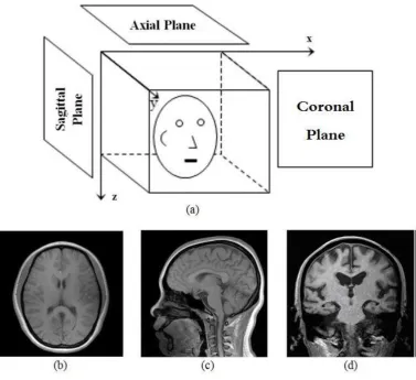
Figure 1.2 MR brain image from patient’s head (a) The setup, (b) Axial plane view, (c) Sagittal plane view, and (d) Coronal plane view (Lorenzen et al. 2001)
Figure 1.3 MR image sequence (Brown and Semelka 2011)
1.3 Background of Research
The medical brain images provide valuable and detailed information regarding normal and abnormal brain tissues. Currently, MR images are the most common test for diagnosing and confirming the presence of brain tumour (Horská and Barker 2010; Joshi 2010; Mehmood et al. 2013). Practically, brain MR images include both normal and abnormal image slices. Despite extensive research, the classification of brain MR image abnormality remains challenging (Padma and Sukanesh 2011; Elaiza et al. 2011a; Al-Badarneh et al. 2012). The resoans are due to variation of possible complex locations, size, shapes, and image intensities for different types of brain tumours (Kikinis et al. 1996; Xu et al. 2002; Veloz et al. 2011; Roy et al. 2013).
and Bora 2014). These diagnoses are based on the location, shape, and image intensity of different types of brain tumours. Clinically, radiologists analyse the brain image slice by slice visually for tumour detection and identification. Such effort is labour intensive, expensive and often erroneous, especially involving a large number of image slices. Furthermore, the sensitivity of the human eye and brain to elucidate such images reduces with the increase of number of cases, particularly when only a small number of slices contain information of the affected area (Salankar and Bora 2014). Therefore, a powerful and reliable tool needs to be developed to automate the tumour localization so that precise detection and segmentation of the abnormal tissue is feasible.
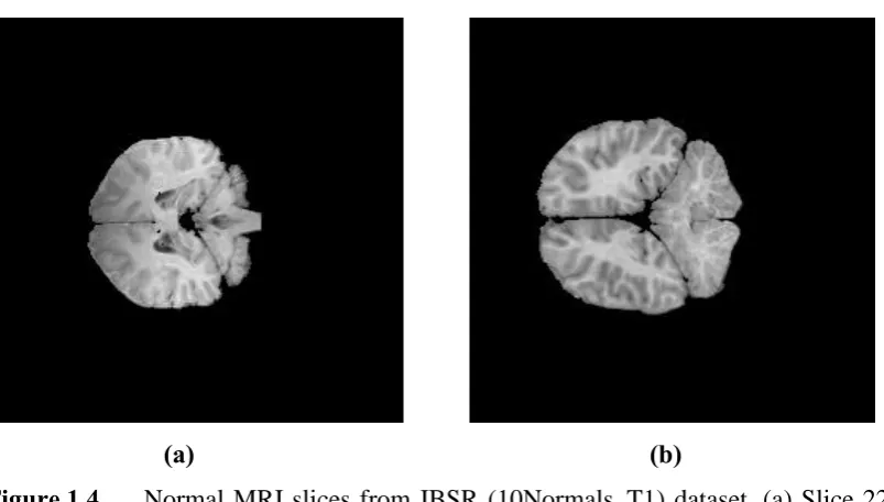
Figures 1.4 and 1.5 display a normal MRI slices of patients. Figure 1.6 illustrates an abnormal MRI slice at different locations, size, shapes, and image intensities for brain tumours in the same patient.
(a) (b)
(a) (b)
Figure 1.5 Normal MRI slices from challenge MICCAI (BRATS2012-BRATS-1) dataset, (a) Slice 119 of patient BRATS_HG0010, and (b) Slice 54 of patient BRATS_HG0008
(a) (b)
Figure 1.6 Abnormal MRI slices at different locations with varying size, shapes, and image intensities of brain tumour (red rectangle) from IBSR (536_T1) dataset of MRI scan 536_32, (a) Slice 22, and (b) Slice 26
present). Separation of these types of these tissues and localization or segmentation of tumours from cerebral tissues poses a severe challenge. Present outcome is far from being satisfactory and radical improvement is necessary (Xu et al. 2002; Harati et al. 2011; Bauer et al. 2011; Wang et al. 2011; Veloz et al. 2011; Hamamci et al. 2012). Figure 1.7 illustrates the separation complexity of the healthy tissues from the cancerous one for challenge MICCAI (BRATS2012-BRATS-1) dataset reflecting the intensity homogeneity and inherent complexity.
(a) (b)
Figure 1.7 Abnormal MRI slices in the presence of tumour inside the red square in terms of intensity homogeneity from challenge MICCAI (BRATS 2012-BRATS-1) dataset, (a) Slice 85 of patient BRATS_HG0004, and (b) Slice 127 of patient BRATS_HG0007
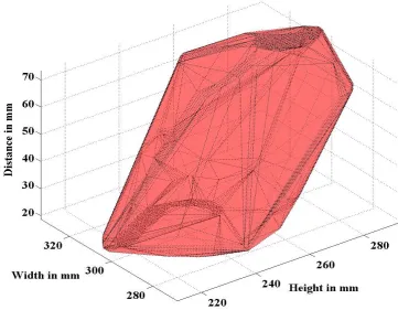
Brain tumour being a well-known serious disease with absolute complexity, the diffusive growth of tumours often makes their resection highly intricate. Usually, surgery is performed to achieve a GTR because the extent of surgical resection determines the longevity of the patient (Lacroix et al. 2001). Indisputably, the graphical visualization is an essential part of brain tumour detection and analysis. Still, accurate brain tumour visualization remains a formidable task. It is crucial to improve the degree of resection for the abnormal tissues while preserving normal tissues (González-Navarro et al. 2012; Yee Lau et al. 2014). Methods are available to visualize the brain tumour, but the major problem with these methods is the inability to visualize the boundaries of the tumour accurately in the details. In addition, their inability to separate the healthy tissues from the unhealthy one leads to the assessment and calculation of wrong tumour volume (Lee 2009; González-Navarro et al. 2012; Yee Lau et al. 2014). Figure 1.8 shows an example of the 3D visualization method of tumour patient, where the actual border is not seen and the tumour does not reveal the difference between healthy and unhealthy tissues.
The estimation of preoperative and postoperative tumour volumes are frequently decided by the surgeon’s impression or on the measurement of its largest axis along x, y and z direction (Lacroix et al. 2001). Precise determination of the brain tumour extent for excised and advanced treatments requires careful calculation and systematic observation of the therapeutic effects on the tumour (Salman et al. 2005; Siegel et al. 2012; Dang et al. 2013). Typically, this is performed by measuring the volume of the tumour from 3D scans. Although, numerous methods for the estimation of the tumour volume are available, but the actual 3D shape of the tumour is seldom displayed. Conversely, each scientific research must evaluate and gauge their result. However, research is not yet perfected to extract the tumour from the brain and measure its volume to validate and evaluate the result given by other related method of brain tumour volume calculation. Simultaneously, there are methods to calculate the brain tumour volume manually. Some of them include Frustum Model (Shally and Chitharanjan 2013), Meshing Point Clouds (Iglesias et al. 2011), Trace method (Chong et al. 2004; Salman et al. 2005) and Modified MacDonald (MMC) method (Dang et al. 2013). However, the results obtained from these methods are not very accurate and often neglects the ground truth. Thus, it is indispensable to uncover an innovative method to gauge and validate the proposed method of tumour volume calculation.
In short, cancer is considered as the disease of the century. Despite the introduction of various methods and calculations the accurate determination of the tumour volume remains unsuccessful and many obstacles still exist that does not allow the full recovery. Moreover, overcoming the uncertainty of these methods in determining the actual volume, the brain tumour shape and the errors in drug dose calculations that lead to wrong dose (over or under) which would finally lead to jeopardizing the human life remain the future challenges. These performance limitations necessitate continued research efforts to mitigate the identified challenges.
MRI slices, brain tumour segmentation, 3D visualization and volume calculation of brain tumour and finally the creation of a new ground truth.
The main issues are how to detect, segment, visualise, and calculate the volume of the brain tumour in MR images with a high reliability?
The specific research questions that need to be answered are:
i) Is it possible to determine brain abnormality accurately?
ii) How to develop a new method to overcome the earlier limitations associated with MRI images brain tumour detection, segmentation, visualization, and volume calculation?
iii) Can the proposed method perfectly segment the brain tumour in MRI images?
iv) Does the new method capable to extract suitable features from the abnormal cerebral tissues which can be used to represent the brain tumour(s) in the MR images?
v) How to determine the brain tumour(s) volume accurately using the extracted features?
vi) Is it possible to represent and visualize the brain tumour in a 3D presentation?
vii) How accurate and reliable the 3D visualization and computed volume of a brain tumour?
viii) How to validate and evaluate the 3D visualization and computed volume of a brain tumour?
1.4 Problem Statements
It is an urgent necessity to build an understanding on the brain tumour detection and subsequent analyses with systematic processing steps, including abnormality detection in MRI slices, segmentation, 3D visualization and volume calculation of brain tumour. Despite numerous available methods satisfactory results on brain tumour detection and segmentation are far from being acquired. Consequently, surgery and diagnostics remain a dispute. Different approaches are proposed for the all previous processing steps. In addition, creation of a new ground truth is mandatory. The entire brain tumour detection scheme mainly depends upon appropriate preprocessing methods in terms of accuracy and reliability. A new fully automatic detection system for brain tumour need to be introduced by taking the following views of the latest developments:
1. Clinically, detection of MRI brain slices’ abnormality is painstaking, voluminous and time-consuming (Singh and Kaur 2012; Kumari 2013; Salankar and Bora 2014). This is due to two main reasons: (1) homogeneity between healthy tissues and cancerous cells, which is very difficult to distinguish even by naked eyes, let alone the machines and, (2) large number of slices involved during the examination - the figure varies whose relies on the type and severity of illnesses (Selvaraj et al. 2007; Abdullah et al. 2011; Salankar and Bora 2014). Thus, many attempts are made to automate the process. However, its performance is rather less impressive and room for improvement is still wide open. Besides, another pressing issue is to localize a tumour or cancerous cell found in the abnormal slice, automatically, which is never being of research interest thus far. Therefore, an effective solution for the above problems not only would equip the doctor with the state of the art, but would also ensure a successful implementation of subsequent procedures, including segmentation, visualization, and volume estimation of tumours in a more precise manner.
2014) because of the variety of possible shapes, locations, and image intensities. The pathology identification, detection of the disease and comparison between normal and abnormal tissues require assorted mathematical algorithms for features extraction, modeling, and measurement in the images. Lately, several useful segmentation algorithms were proposed (Moon et al. 2002; Zacharaki et al. 2008; Farmaki et al. 2010). However, due to the nature of tumour, the accuracy of the algorithms is far from satisfactory (Dass and Devi 2012; Shin 2012; Roy et al. 2013).
3. Another pressing issue on tumour treatment is accurate 3D visualization of the tumour. However, research interest in this area is very limited (Wu et al. 2008; Lee 2009; González-Navarro et al. 2012; Wakchaure et al. 2014). Unfortunately, the accuracy of their works is challengeable due to the absence of the ground truth to validate their results (Wakchaure et al. 2014). Also, most of the tumour shapes generated by the methods are far from satisfactory because they only provide gross shape of the tumour, let alone to distinguish between the healthy tissues and cancerous tissues (Wakchaure et al. 2014).
4. In the cancer treatment, the tumour volume plays a significant role in determining the recommended therapy (Shi et al. 1998; Nelson 2001; Dubey et al. 2009; Shally and Chitharanjan 2013; Mehmood et al. 2013). In spite of several methods for tumour volume calculation such as Meshing Point Clouds, Frustum Model, Trace Method and Modified MacDonald (MMC) the detection accuracy and reliability remains debatable due to the absence of the ground truth to validate the findings (Lau et al. 2005; Shally and Chitharanjan 2013). Actually, these methods fail to determine the actual size of the tumour (Shally and Chitharanjan 2013). Therefore, a precise volume calculation method is required to overcome these drawbacks.
1.5 Research Goal
The goal of this thesis is to develop a new MRI brain tumour detection system, which includes brain tumour detection, segmentation, 3D visualisation and volume calculation, with a higher degree of accuracy than the existing one.
1.6 Objectives of the Study
In order to achieve the above mentioned goal, the following objectives need to be accomplished:
1. To detect the abnormal slices of the MR brain images.
2. To propose a new segmentation technique using the Slantlet Transform (SLT) that can precisely localise the brain tumour from cerebral tissues. 3. To develop new techniques for 3D visualization and volume calculation
of the brain tumour based on the Alpha (α) shape theory.
4. To create two ground truth s for 3D visualisation and volume calculation of MRI brain tumour, respectively.
1.7 Research Scope
tumour. Computer experiments will be performed to test the proposed system on three standard datasets. The first two datasets are obtained from the Internet Brain Segmentation Repository (IBSR) created by the Center for Morphometric Analysis, Massachusetts General Hospital (USA), named IBSR (10Normals_T1) without any brain tumour and IBSR (536_T1) with brain tumours. They are used by several researchers for brain tumour detection worldwide. The third dataset called challenge MICCAI (BRATS2012-BRATS-1). The Multimodal Brain Tumour Segmentation (BRATS) challenge was the 15th international conference on Medical Image Computing and Computer Assisted Intervention (MICCAI 2012) held in France (2012). This datasets provides a large number of brain tumour MRI scans in which the brain tumour regions have been manually delineated.
This study will mainly focus on T1-weighted High-Grade (HG) brain tumour in three planes (axial, coronal, and sagittal plane) for MR image segmentation, 3D visualization and volume calculation of elevated category. However, the Low-Grade (LG) tumour and tumour classification either benign or malignant are beyond the scope of the present thesis. In addition, another MRI pulse sequences such as T2-weighted, PD-weighted (Proton Density), and Fluid-Attenuated Inversion-Recovery (FLAIR) are not within the scope.
1.8 Significance of the Study
precise segmentation for the brain tumour by reducing segmentation error, resolve problems associated with tumour volume calculation, and visualize the brain tumour in 3D shape, and give a new way to create a new ground truth. In light of the above mentioned issues, the results of this research will contribute to what is currently known about brain tumour detection systems. Nonetheless, the significance of this study is not only limited to knowledge enrichment, but also to the development of a new method for future implementation and brain tumour diagnosis and cure.
1.9 Thesis Outline
This thesis is organized as follows. The rest of the chapters begin with a brief description highlighting the aims of each chapter and ends with a short summary. Each chapter is developed to be self-contained, but there exists cohesion among the chapters in order to ensure the free flow of presentation and understanding of the thesis content. It should also be borne in mind that mathematical notations and definitions are introduced at various points to render a consistency and better understanding of the presentation.
Chapter 3 presents a clear roadmap of this study to guide the reader for quick grasp of the detailed research framework. The advantages of using the popular dataset in the newly developed methods are emphasized. The layout of the entire research framework, strategies, and procedures are highlighted.
Chapter 4 discusses the proposed methods in details. It covers the cerebral tissue extraction, slice abnormality detection, segmentation, 3D visualisation and volume calculation of the MRI brain tumour.
Chapter 5 provides the experimental results, detailed analyses, and discussions. It explains the qualitative and quantitative measurements that are carried out for the performance evaluations and implementation of the method for every single phase such as detection of the MRI slices abnormal, segmentation of brain tumour, brain tumour 3D visualization and volume calculation. The qualitative measurements are based on visual human inspections, while the quantitative measurements are performed using standard approaches. In addition, every process is benchmarked against the best and up-to-date techniques for segmentation and volume calculation found in the literature.
REFERENCES
Abdullah, H. N., and Ali, S. A., (2010). Implementation of 8-Point Slantlet Transform Based Polynomial Cancellation Coding-OFDM System Using FPGA. 7th International Multi-Conference on Systems, Signals and Devices, pp.1–6.
Abdullah, N., Ngah, U. K., and Aziz, S. A., (2011). Image Classification of Brain MRI Using Support Vector Machine. Imaging Systems and Techniques (IST), IEEE International Conference, pp. 242–247.
Aboutanos, G. B., Nikanne, J., Watkins, N., and Dawant, B. M., (1999). Model Creation and Deformation for the Automatic Segmentation of the Brain in MR Images. Biomedical Engineering, IEEE Transactions, vol.46, no.11, pp.1346–1356.
Adams, R., and Bischof, L., (1994). Seeded Region Growing. Pattern Analysis and Machine Intelligence, IEEE Transactions, vol.16, no.6, pp.641–647.
Al-Badarneh, A., Najadat, H., and Alraziqi, A. M., (2012). A Classifier to Detect Tumor Disease in MRI Brain Images. Advances in Social Networks Analysis and Mining (ASONAM), IEEE/ACM International Conference.pp. 784–787. Alia, O. M., Mandava, R., and Aziz, M. E., (2011). A Hybrid Harmony Search
Algorithm for MRI Brain Segmentation. Evolutionary Intelligence, vol.4, no.1, pp.31–49.
Al-Kadi, O. S., (2010). Assessment of Texture Measures Susceptibility to Noise in Conventional and Contrast Enhanced Computed Tomography Lung Tumour Images. Computerized Medical Imaging and Graphics, vol.34, no.6, pp.494– 503.
Amrutal, A., Gole, A., and Karunakar, Y., (2010). A Systematic Algorithm for 3-D Reconstruction of MRI based Brain Tumors using Morphological Operators and Bicubic Interpolation. Computer Technology and Development (ICCTD), 2nd International Conference on. IEEE. pp.305–309.
Angelini, E. D., Delon, J., Bah, A. B., Capelle, L., and Mandonnet, E., (2012). Differential MRI Analysis for Quantification of Low Grade Glioma Growth. Medical Image Analysis, vol.16, no.1, pp.114–126.
Antonie, L., (2008). Automated Segmentation and Classification of Brain Magnetic Resonance Imaging. C615 Project, pp.1-15.
Ariffanan, M. and Basri, M., (2008). Medical Image Classification and Symptoms Detection Using Neuro Fuzzy. Universiti Teknologi Malaysia, Faculty of Electrical Engineering, Malaysia.
Aurdal, L., (2006). Image Segmentation Beyond Thresholding. First Edition. Norsk Regnescentral.
Avision, J., (1989). The World of Physics. Second Edition, Thomas Nelson and Sons. Badran, E. F., Mahmoud, E. G., and Hamdy, N., (2010). An Algorithm for Detecting
Brain Tumors in MRI Images. The International Conference on Computer Engineering and Systems. IEEE, pp. 368–373.
Baillard, C., Hellier, P., and Barillot, C., (2001). Segmentation of Brain 3D MR Images Using Level Sets and Dense Registration. Medical Image Analysis, vol.5, pp.185–194.
Balafar, M. A., Ramli, A. R., Mashohor, S., and Farzan, A., (2010). Compare Different Spatial Based Fuzzy-C_mean (FCM) Extensions for MRI Image Segmentation. Computer and Automation Engineering (ICCAE), The 2nd International Conference. IEEE. pp. 609–611.
Balafar, M. A., (2012). Gaussian Mixture Model Based Segmentation Methods for Brain MRI Images. Artificial Intelligence Review, pp.429–439.
Balafar, M. A., Ramli, A., and Mashohor, S., (2011). Brain Magnetic Resonance Image Segmentation Using Novel Improvement for Expectation Maximizing. Neurosciences, vol.16, no.3, pp.242–247.
Bauer, S., Nolte, L. P., and Reyes, M., (2011). Fully Automatic Segmentation of Brain Tumor Images Using Support Vector Machine Classification in Combination With Hierarchical Conditional Random Field Regularization. Medical Image Computing and Computer-Assisted Intervention : MICCAI. pp. 354–361.
Berg, M. D., Cheong, O., Kreveld, M. V., and Overmars, M., (2000). Computational Geometry - Algorithms and Applications. Second Edition, Springer.
De B., Mark, C., Otfried, V. K., Marc, O., (2008). Delaunay Triangulations. Algorithms and Applications. pp.191–218.
Bermel, R. A., Sharma, J., Tjoa, C.W., Puli, S. R., and Bakshi, R., (2003). A Semiautomated Measure of Whole-Brain Atrophy in Multiple Sclerosis. Journal of the Neurological Sciences, vol.208, no.1-2, pp.57–65.
Bezdek, J. C., Ehrlich, R., and Full, W., (1984). FCM : The Fuzzy c-Means Clustering Algorithm. Computers and Geosciences, vol.10, no.2, pp.191–203. Birkbeck, N., Cobzas, D., Jagersand, M., Murtha, A., and Kesztyues, T., (2009). An Interactive Graph Cut Method for Brain Tumor Segmentation. Workshop on Applications of Computer Vision (WACV), pp.1–7.
Blanton, R. E., Levitt, J. G., Peterson, J. R., Fadale, D., Sporty, M. L., and Lee, M., (2004). Gender Differences in the Left Inferior Frontal Gyrus in Normal Children. NeuroImage, vol.22, no.2, pp.626–636.
Boesen, K., Rehm, K., Schaper, K., Stoltzner, S., Woods, R., Lüders, E., and Rottenberg, D., (2004). Quantitative Comparison of Four Brain Extraction Algorithms. NeuroImage, vol.22, no.3, pp.1255–1261.
Bourouis, S., and Hamrouni, K., (2010). 3D Segmentation of MRI Brain Using Level Set and Unsupervised Classification. International Journal of Image and Graphics, vol.10, no.1, pp.135–154.
Bronnikov, A. V., (2012). SPECT Imaging With Resolution Recovery. IEEE Transactions on Nuclear Science, vol.59, no.4, pp.1458–1464.
Brown, M. A., and Semelka, R. C., (2011). MRI Basic Principles and Applications, Fourth Edition, Hoboken, New Jersey: John Wiley and Sons, Inc.