Approximate analysis of arbitrary configurations of queueing networks with blocking and deadlock

BLOCKING AND DEADLOCK

l

I

K.P.

JUD

Operations Research Program and

Center for Communications and Signal Processing and

H.G.

Perros

Computer Science Department and

Center for Communications and Signal Processing North Carolina State University

Raleigh, NO 27895-8206

CCSP-TR-88/11 March 1988

1. Introduction

Studies of arbitrary configurations

or

open queueing networks with blocking

have been reported in the literature. Below, we review briefly the relevant

litera-I

ture using the classification scheme of blocking mechanisms reported in Onvural

and Perros[8]. Takahashi, Miyahara, and Hasegawa{11] developed an

approxima-tion procedure for analyzing such networks under type 1 blocking mechanism.

They assumed that the effective service times of servers liable to getting blocked is

exponentially distributed. Boxma and Konheim[3] studied three basic

configurations with a view to developing an approximation algorithm for the

analysis of such arbitrary queueing networks under type 2 blocking mechanism. Labetoulle and Pujolle{7] and Kerbache and Smith[6] analyzed open

nonexponen-tial queueing networks with blocking using a diffusion approximation under type

3.1 blocking mechanism. They assumed that the arrival process at each queue is a renewal process. Yao and Buzacott[12] reported on an approximation algorithm for

analyzing closed queueing networks under blocking mechanism type 3.2, assuming

Coxian service times and reversible routing. Altiok and Perros{2] presented an

approximation algorithm for analyzing feed-forward configurations of open

exponential queueing networks with blocking under type 1 blocking mechanism.

The

effective service time

at

each node was approximated by a phase-type distribu-tion representing all possible blocking delays. This algorithm works for small

net-works because of its complexity. Perras and Snyder[lO] presented a

Perros[2). They used two-phase Coxian distributions for approximating the effective service times, thus reducing the amount of computation considerably.

The analysis of arbitrary configurations of open queueing networks with

I

blocking and deadlock has not been yet reported in the literature. In this paper,

we present an approximation algorithm for analyzing arbitrary configurations of

open exponential networks with type 1 blocking. Unlike other approximation

algorithms, the proposed algorithm takes into account the problem of deadlock.

The queueing networks considered here consist of finite queues arbitrarily

intercon-nected. In view of this, blocking of different queues may cause deadlocks. Deadlocks are assumed to be detected and resolved instantaneously. This class of

queueing networks is described in detail below.

2. Open Queueing Networks with Blocking and Deadlock

The open queueing networks with blocking and deadlock we consider here

consist of finite single server queues linked arbitrarily. Figures 1 and 5 show such

networks. There is an external arrival process to each node. All service times and

interarrival times are assumed to be exponentially distributed. Units in each queue

are served in FCFS manner. Only one class of units is considered.

The

capacity of all queues is finite.

I

Figure 1. The 3-node network

blocking unit is forced to wait at queue i until it enters queue j. During this time the ith server is blocked and it cannot serve any other units that might be waiting

in its queue. Now, let us assume that there are m queues directly linked to queue

i.

Then it is possible that at any time there might be more than one blocking unit

waiting to enter queue j. The total number of blocking unitsmay not exceed m. It

is assumed that these blocking units enter queue j on a firat-blocked-ftrst-enter basis. An external arrival to a node isassumed to be lost ifthe queue is full.

Due to the blocking mechanism described above and the arbitrary

intercon-nection of the queues, deadlock may occur. For example, suppose that node i is

will occur. It is assumed that a deadlock is detected and resolved instantaneously.

In this paper, it is assumed that a deadlock is resolved by simultaneously

I

exchanging blocking units(see [9]). In general, this scheme for resolving deadlocks

may violate the first-blocked-first-enter priority rule described above. For instance,

suppose that queue i and k are blocked by queue 1- in that order. That is, if a departure occurs from queue j, the blocking unit from queue i will enter queue j

first. Let us now consider the following situation: suppose that the departing unit

from queue 1- chooses queue k as its destination and that queue k is

full

at that moment. This causes a deadlock to occur. The deadlock is resolved by simultane-ously exchanging the blocking units Cram queue k and queue j. In view of this, the

blocking unit from node k enters node J. first and node i still remains blocked by

node j -Thus, the first-blocked-first-enter priority rule has been violated.

The algorithm described in this paper is built upon the algorithm reported by

Altiok and Perras [2] as it was further developed by Perros and Snyder{lO]. In par-ticular, it decomposes the queueing network under study into individual queues,

each with a revised arrival and a revised capacity. Each queue is then studied in isolation. The parameters of each queue are revised as follows:

a) revised arrival process: Each queue has an external arrival process and one

internal arrival process per upstream node. Each internal arrival process is

b) revised service process: The service process of each server is characterized by a

phase-type distribution, whose parameters reflect all the possible blocking

delays and deadlocks.

I

c) revised capacity: The capacity of each queue is augmented by as many

posi-tions as the number of the queues directly linked to this particular queue.

This is necessary because the blocking mechanism considered here allows a

blocked server to act as an additional buffer space for the blocking queue.

The approximation algorithm is presented in the following section, and it is

validated in section 4. The conclusions are given in section 5.

3. The Approximation Algorithm

For presentation purposes, we describe the algorithm in detail as applied to

the smallest arbitrary configuration (but by no means trivial) of the queueing net-work. This queueing network consists of three nodes as shown in figure 1. Let A.o',

J.Li' and

N,

be respectively the external arrival rate of customers, the service rate,

and the capacity of queue i (including the one in service), for i

=

1,2,3.

In order to study each queue in isolation, we first augment the capacity of

queue i by two, seeing that queue i has two upstream nodes. Also, each queue has an external arrival stream and two internal arrival streams. It is assumed that the

two internal arrival processes are Poisson processes.

The service mechanism of each queue is revised by considering all the possible

blocking delays and deadlocks. The resulting effective service of queue 1 has the phase-type representation shown in figure 2, which is explained in detail below.

I

For queues 2 and queue 3, the service mechanisms can be constructed in the same

ways as in queue 1.

Let us now focus on queue 1. A unit starting its service first receives an

exponentially distributed service with mean I/JL1. The unit may, upon service

completion at queue 1, either leave the queueing network with probability riO or

choose to enter queue 2 or queue 3 with probability r12' r13 respectively. Let us assume that the unit goes to queue 2. If queue 2 at this moment is not full, no

blocking delay occurs. Otherwise, the unit going from queue 1 to queue 2 may find

either queue 2 Cull, or queue 2 full and a blocking unit(from queue 3) already wait-ing to enter queue 2. This is indicated by events {F(1,2)

&

S(3)*2}

and

{F(l,2)

&

S(3)=2}

respectively in figure 2, where

F(i,j)

indicates the event that an arriving

unit from node i finds node j full, and

S(i)=

j indicates the event that server i is

busy if i

=

i,

or server i is blocked by node j if i=1=j. The total blocking delay depends on the state of server 2.

In the first event,

{F(1,2)

&

S(3):;e2},

there are three possible states of server 2 at the time when server 1becomes blocked by queue 2:

(a) If server 2 has been already blocked by queue 1,

{S(2)=

I}, a deadlock occurs,

which is resolved by exchanging the blocking units simultaneously. In this case, no

5(3)=1 DL

(1.3) &1

5(2)=3 r_{1 0}

N8 _f\B

NF(2.1 )N3

NF(1,2) r21

N8

L

l

G:

,

JJ._{2 /}

F(1,2) &S(2)=2

r,2 (3)=2

,

5(2)=3 _S(31=~ ~

r_{3 1} NF'3.1)r£

~E(3.1)

Dl F(3.1)

CL

r 0

32 ~L--G. r3 2

J..L, G, DL-G~

F(2.1 )

NF(1,3)

i'I3

r_{2 3}

--a

I

r₂₀ r

13

NOTATION F (L,j) NF(i,j) S(i)=j

NB

DL Gl

An arriving unit from i finds j full An arriving unit from i finds j not full

Server i is busy if i~j

Server i is blocked by j if 1;j No blocking delay

Deadlock

Repeating event

(b) If

server 2 is

busy,

{S(2)=2},

then the blocking unit in queue

1

suffers a delay denoted by G1. In particular, the blocking unit will be blocked for an exponential

amount of time with mean I/J.L2. Following service completion at server 2, this

I

server may in turn get blocked by queue-S if the departing unit with probability

r23 chooses to go to queue 3 and queue 3 is full at that moment, which is the event

{F(2,3)}.

Now, if server 3 is already blocked by queue 1,

{S(3)=

I}, then a

deadlock occurs which is resolved instantaneously, and thus no blocking delay occurs. If server 3 is blocked by queue 2,

{S(3)=2},

a deadlock also occurs

involv-ing queues 2 and 3.

In

this case, the deadlock is resolved by simultaneously exchanging the blocking units in queues 2 and 3, which causes the unit at queue 1 to be further blocked from entering queue 2. The remaining blocking delay isgiven by G_{t .}

In

the last case,

{S(3)=3},

the blocking unit in queue 1will be blocked for an additional exponential amount of time with mean I/J.L3. After service

comple-tion at server 3, the unit may either leave the network or it may choose to enter queue 1 or queue 2. II it leaves the network, a buffer space at queue 3 becomes available and then server 1 and server 2 become unblocked. If that unit attempts

to enter queue 1, server 1, 2 and 3 become unblocked whether queue 1 is full or not. A deadlock occurs if it attempts to enter queue 2. Upon resolution of the deadlock server 2 becomes unblocked, but server 1 is still blocked. The remaining blocking delay is given by G1.

{S(3)=2} is not possible. In the event {S(3)=

I},

we have a directed cycle consist-ing of queue 1, queue 2, and queue 3. This means that a deadlock has occurred. In

the event {S(3)=3}, the blocking unit in queue I

will

be blocked for the remaining

I

service time of the unit being served by server 3, which isexponentially distributed with mean l/fJ.3. If this unit attempts to enter queue 2 then a deadlock occurs between queue 2 and queue 3.

By

exchanging the blocking units from queue 2 and queue 3, server 1 is still blocked and server 2 becomes busy. This means that the blocking unit in queue 1will be further delayed by G1.

In the event denoted

by {F(1,2)

& S(3)=2}, there are two possible states of server 2, i.e., {S(2)= I} and

{S(2)=2}.

Now, in the case {S(2)= I}, a deadlock

occurs between queue 1 and queue 2. When server 2 is busy, {S(2)=2}, the

block-ing unit from queue 1 will be blocked for the remaining service time of server 2,

which is exponentially distributed with mean I/J..L2. The unit upon service

comple-tion at server 2 either leaves the network with probability f20 or chooses to enter

queue 1 or queue 3 with probability r21 and '23 respectively. If this unit leaves the

network a buffer space becomes available at queue 2 and the blocking unit from

queue 3 enters queue 2. The blocking unit from queue 1will be blocked by

G

1. In the other case, where the unit upon service completion at queue 2 goes to queue 3,

there will be either a deadlock between queue 2 and queue 3, or server 3 will

become unblocked, depending on whether queue 3 is full or not. The resulting

blocking delay of the blocking unit from queue 1 is given by G_1•Finally, ifthe unit

either a deadlock occurs between queue 1 and queue 2, or the unit from queue 2

enters queue 1 depending upon whether queue 1 is Cull or not. Consequently, in

the latter case, server 3 becomes unblocked first and as a result, server 1is delayed

I

by

G

1. In the former case, there is no additional delay.

When a unit upon service completion at queue 1attempts to enter queue 3 the phase-type structure of the effective service at queue 1 can be obtained by similar

arguments. Furthermore, the effective service process of queue 2 and queue 3 can

be obtained in the same way as in the case of queue 1. Now, we proceed to

deter-mine allthe branching probabilities in figure 2.

3.2. The Branching Probabilities

Let us consider one of the queues of the three-node queueing network, say

queue i . (For presentation purposes, we shall refer to the other two queues as

i

and

k.)

Now, let us suppose for the moment that all the branching probabilities of queue i's effective service time are known. Then, we can construct a simpler form

of this phase-type distribution by collapsing parts of it into Coxian-2 distributions

using the three-moment approximation technique(see

[1]).

In particular, the part of

the phase-type distribution that represents the blocking delay due to queue

i

is

collapsed into a Coxian-2 distribution, We do likewise for the part of the

phase-type distribution that represents the blocking delay due to queue k . The resulting

section.

Now, we show how the branching probabilities are determined. We introduce

the following parameters:

I P(E) the probability of occurring an event E

~ii the effective arrival rate from queue i to queue j

•

l/J.Li the mean effective service time of server i

1t'ii

(n

,1) the conditional probability that upon service completion at server I, there are n units at queue j and server j is at phase 1

R_il the remaining service time

of

server i

at

phase 1 Pi(O) the steady-state probability that queue i is empty

Pi(m,n

,I)

the steady-state probability that queue i is in the state

(m .

n ,1)

Queue i has the following state space:

E

=

{O,( m,n,1); m =0,1, n

=

1,....N,

+

2, 1=I, ...,S},

where n is the number of units(including the one in service) at queue i, I is the state of server i ,and m is an indicator variable used to describe who is blocked by

queue i . Because of the first-blocked-first-enter priority rule, we need to keep track

of the order in which upstream queues become blocked by queue i . The states or

queue i and their description are summarized in table 1.

State

o

(O,n

,l),l~n< N,

(O,Ni

+

1,1)

(I,Ni+1,/)

(l,Ni

+

2,1)

(O,Ni+2,1)

Description server i is idle

no one is blocked by queue i , there are n customers in the queue and server i is at phase I

queue k is blocked but queue J. is not blocked by queue i

queue j is blocked but queue k is not blocked by queue i

both queues are blocked by queue

i;

queue j first and queue k next in

ord-er

both queues are blocked by queue i; queue k first and queue j next in

ord-er

NOTE: 1)

i*i,Jc

and j

<k

2) I

=

1;server i is busy

1=2,3; server i isblocked by JO I=4,5; server i is blocked by

Ie

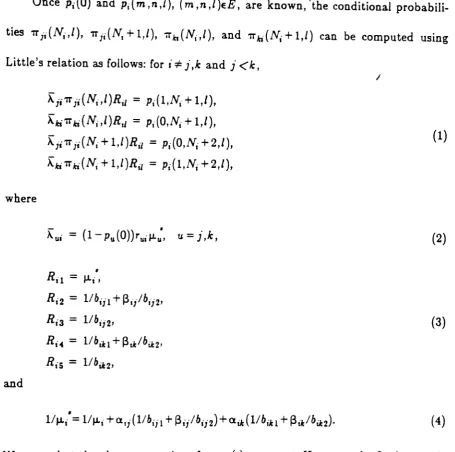
Once

Pi(O)

and pi(m,n,l), (m,n,I)EE, are known, "the conditional probabili-ties

'TT'jdNi,l), 'TT'ji(NI+l,l), ir/n(Nj,I),

and

'TT'/n(Nj+l,l)

can be computed using Little's relation as follows: for i=l=

i,k

and j

<k,

I

where

and

~ji7rji(Ni,l)Ril= _Pi(l,Ni+1,1),

~a7Tki(Ni,I)Rd

=

Pi(O,N_i

+

1,1),

~iiTrji(Ni+l,I)Ril

=

_pi(O,Ni+ 2,1),

~hTrki(Ni+1,I)Ril

=

Pi(I,N..

+

2,1),

,

R'_tl = I I ·_{r t ,}

Ri 2

=

1/bii 1

+

~iilbij2'

R"3

=

l/b·°2

t

I' '

Ri~

=

I/bik 1

+

~iklbik2'

RI"s

= 1/bik 2,

,

1/J.Li

=

1/ JLi

+

Clti (1Ibi j1

+

~iiibii2)

+

CliJc (1/bile1

+

J3ile /biJc2) •

(1)

(2)

(3)

(4)

We note that the above expressions for rr., (.) are exact. However, the final

numeri-cal values for 7r.j ( .) are approximate seeing that Pi (.) are obtained approximately.

Using the above Pi'5 and 1T.i'S, we can calculate approximately the branching

probabilities. For example, consider the event

{F(1,2)

& 8(3);=2

&

S(2)=2}

in figure 2. This event occurs when a unit from queue 1 arrives at queue 2 to find

queue 2° full, queue 3 not blocked by queue 2, (i.e., N₂ units in queue 2) and server

S(2)=2)=n12(N

₂,1). For the event {F(1,2)

&

8(3)=2 &

S(2)=2},

where

a

unit from queue 1 arrives at queue 2 to find queue 2 Cull, a unit from queue 3 waiting to enter, and server 2 busy, the probability is

P(F(1,2)

& 8(3)=2

&

I

Until now, we showed briefly how the effective service mechanism shown in

figure 3 can be obtained. For further details, see [5]. In the next section, we explain how to compute the steady-state queue length distribution of each queue.

3.3. The Steady-State Queue Length Distributions

We obtain the steady-state queue length distribution of each queue numeri-cally. From this other performance measures can be computed. We define the state space, generate the rate matrix Q and then solve the linear system QTx=0, where z is the probability vector. The state space of each queue was defined in the previous section (see table 1). The rate matrix

Q

of queue 1 for N_l=2, for instance, is shown in figure 4. In matrix QJ we have two unknown parameters, A21

and A311 which are the overall arrival rates from queue 2 and queue 3 respectively

to queue 1. In general, the two unknown parameters, Aii and Alei

(i

*

j ,k and

j <k), are determined iteratively from two fixed-point problems,

(5)

and

(6)

5

pi(m,n)

=

2:pi(m,n,I).

1=1

For each value of Aji and Ah, the linear system, QT%=0,was solved using the

I

successive over-relaxation(SOR) algorithm (see

[4], p.357).

0 1 2 3 4 5 6

0 -AI Al 0

a

0 0 0

1 8° S-A1I All

a

0 0

a

2 0 So

TO

S - (A31

+

A21)I A31 I A'l1I 0 0

Q=

0 0 So

TO

8-A2lI 0 0 _A211

3

4 0 0 So

TO

0 S - A31I A311

a

5 0 0 0 So

TO

0 S

a

6

°

0 0 0 So

TO

0 8

where

So

=

(QI0J.Ll,(1-

~12)b

121'b122'(1-

~13)b

131'b132)T,

TO

=

(1,0,0,0,0),

- JoLI Cl12JLl

°

ex13J.Ll 0

0

-°

_{12 1} r312b121 0 0

s=

0 0 - °122 0 0

0 0 0 - °131 ~13b131

0 0 0 0 - °132

and

Al

=

AOI

+

A21

+

A31-Note; 1:(0,1,1), 2:(0,2,1), 3:(0,3,1),4:(1,3,1), 5:(1,4,1),

3.4. The Algorithm

We now proceed to describe the approximation algorithm used to obtain the

queue length distribution of each queue. The algorithm is an iterative scheme and

I

it is similar in spirit to the isolation method due to Labetoulle and Pujolle[7].

In

particular, we analyze each queue separately using the methodology described

above. An iteration is completed when every queue in the queueing network has

been analyzed. Following a convergence test we may stop or carry out another

iteration. The order in which we analyze each queue within an iteration is not

important. Furthermore, within each iteration, in order to analyze a queue we

need to have certain values from the other queues of the queueing network. For the

queues that already have been visited during this iteration, we use the new

updated values. For those queues that have not been visited yet, we use the values

obtained from the previous iteration. Below, we summarize this algorithm for the

three-node network.

Initialization Step

For each queue i , i

=

1,2,3,

1. Give arbitrary values to the parameters of the phase-type distribution of the effective service time shown in figure 3, and also to the effective internal arrival rates

x:!:),

U

=

[.k .

2.

Obtain

RJO)

and "",/(0) using

(3)

and

(4).

3. Calculate Pi(O), Pi(O)(m,n,l) using the above numerical procedure, and obtain piO)( n), n

=

1,2,....N,

+

2, where Pi(O)(n)= LLPi(O)(m,n

,I).

m I

Iteration Step

1.

2.

3.

4.

5. 6. ,.,

,

"

8.

For queue ., i

=

1,2,3,

Compute

~~),

tL

=

j,k, using (5) and

(6).

Calculate all the branching probabilities of the complete phase-type

represen-tation of its effective service time, shown in figure 2. Using the method of moments, collapse this distribution to the simplified phase-type distribution

shown in figure 3.

Obtain

RJl)

and

J-L/(ll.

Analyze queue i using the numerical procedure described In section 3.3,

obtain

pP)(O)

and

ppl(m,n,l).

Calculate ~(I) and obtain 11'(1)(.)and 1T(~)(e) u=Je k

lU , au U I " •

C

t \ (I) _ . k e (1)( I)

ompu e I\.ui , u - ), ,usIng Pi m,n , .

Ifmaxl~(q)-A(~)I<E_{UI U I '} goto8 Otherwise set~(~)=~(~) p.(O)(.)=p.(I)(e) and zo

e ' U I UI' I I ' 0

U

to 2.

Set ~_1U(o)=~_IU'(1) 11'(O)(

e)

=

11' (1)(

e)

and 11'(~)(.)

=

11"(~)(.) U

=

J" k

II' a u ' UI U I ' , .

Convergence Step

1. Calculate

pP)(n)=2:2:pp)(m,n,I), n=1,2,...,N

j+2.

m I

2. Test if maxlp/O)(n)-pp)(n)l<e,

n=O,1,...,N

j + 2 , ;=1,2,3. Ifyes, then stop.

i,rI

Otherwise, set

Pi(O)(n)=pp)(n), n=O,l, ...,N

j + 2 , ;=1,2,3, and repeat the

iteration step.

It should be noted that the actual probability of Pi(N_{i )} IS the sum of Pi(N_{i ) ,}

From the steady-state queue-length distribution Pi

(n),

we can calculate

several measures of performance such as the throughput (THj ) , the server

TH_i

=

(1-

Pi

(0)

)J.LI-= ~~tJ&

+

AOi(l-Pi(Ni ) )

u*i

u·

_I

=

I-pi(O) N,

L·1

=

~npi(n).

",=0

(7)

I

4. Numerical Examples

The approximation algorithm discussed in section 3 was implemented on a

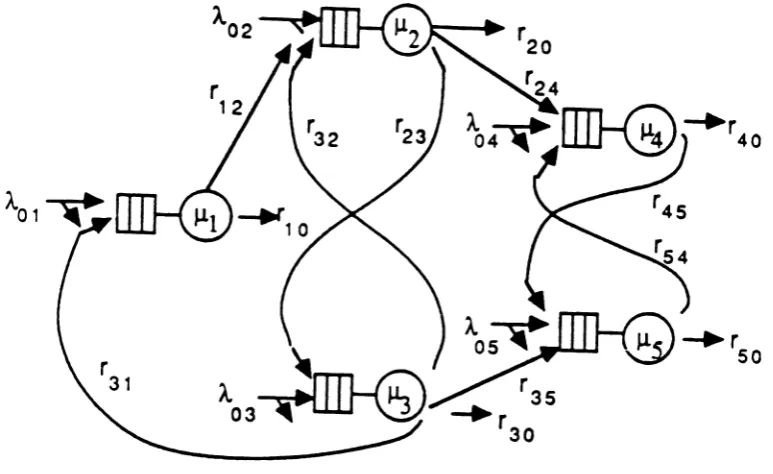
VAX 11/785 to analyze the three-node network shown in figure 1 and the five-node

network shown in figure 5. The main results obtained are the steady-state queue

length distributions for each queue. From this information, other more commonly

sought performance measures, such as throughput, server utilization, and mean

queue length, can be obtained. The approximate results were compared with

simulation results. Each simulation run comprised of at least 200,000 departures.

The results are summarized in tables 2 to 9. In particular, tables 2 to 5 give

results for the three-node network, and tables 6 to 9 give results for the five-node

network. Each table gives the probability that the server is idle, the probability

that the queue is full, the mean queue length, and the throughput of each queue.

Finally, each table also give relative errors and the cpu time used by the

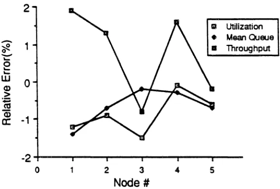
approxi-mation procedure. For presentation purposes, figures 6 to 9 give plots of the

rela-tive error of the approximate results for the server utilization

(U

_{i ) ,} throughput

( THi ), and mean queue length (Li )of each queue, for some of examples reported in

I

Figure 5. The 5-node network

The proposed algorithm gives, In general, good results. The approximate results for the throughput and mean queue length have a relative error less than 5%. Also, most of the approximate results for the queue-length distributions have a relative error less than 10%. Some of the approximate queue-length probabilities have a relative error as high as 20%. However, these cases are not significant,

see-ing that the probabilities are quite small. For more validations see [5].

In this paper, we described an approximation algorithm for obtaining the

queue-length distribution of arbitrary configurations of open queueing networks

with blocking and deadlock. The approximation procedure was built upon the

I

algorithm reported by Altiok and Perros[2] and Perras and Snyder[lO]. In

particu-lar, it decomposes the queueing network into individual queues with revised queue

capacity and revised arrival process and service process. These individual queues

are then analyzed in isolation. The service mechanism of each server that is liable

to get blocked is modified in order to accommodate all the possible blocking delays

and deadlocks. The resulting service mechanism is of the phase-type, whose

parameters are obtained iteratively. The algorithm has a satisfactory error level.

However, it requires the construction of very detailed phase-type service mechan-isms, which is rather time consuming. Further work, therefore, is required to

alleviate this problem.

Finally, we note that, in this paper, we assumed that a deadlock is detected

and resolved instantaneously. However, this assumption may not be the case in

real-life systems. In fact, it is more likely that detection and resolution may require

o

-1

Utilization M8CW'1 OJeue Throughput

I

3 2

-2

-r----r---r----...---o

Node #

Figure 6. Relative error(%) for U_{i ,} L_{i ,} and TH,

(Data are given in table 2.)

2

a Utilization

...-... 1

•

Mean Queue

~

0

•

_Throughput

...,

~

0 0

~

'

-W

Q)

> -1

' : ;

as (j)

a:

-2

-3

0 2 3

Node #

Figure 7. Relative error(%) for

v.,

t.;

and TH1

3

2 II Utilization ..-..

•

MeanQueue I

~

0

1

•

Throughput ..., ~ 0 ~ ~ W 0 C1l > . ' ; as _-1 <D a: -2 -3

0 2 3 4 5

Node#

Figure 8. Relative error(%) for

o..

i;

and THi

(Data are given in table 6.)

o

2 ~ o ..., ~ o ~ ~

w

Q) > :;:: ca Q3 a: -1 Utilization Mean Queue Throughput 5 4 2 3 Node #

-2t..,...,...,...

-o

Figure 9. Relative error(%) for U_{i ,} L_{i ,} and THi

Table 2. AO= (1.5,2.0,1.8); ~=(3.0,4.0,3.5); N=(3,3,3);

"ic=0.5,r 12=0.3,r13

=

0.2,r20=0.5,r21

=

0.2,T23

=

0.3,r30

=

0.5"31

=

0.3,r32=0.2;

cpu

=

7.3 sec

Approximate Simulation Rel.Error

Pl(O)

0.202 0.194 0.041

pt(3)

0.366 0.367 -0.003

L₁ 1.750 1.768 -0.010

TH₁ 2.167 2.177 -0.005

P2(O)

0.247 0.24"2 0.021

P2(3)

0.303 0.296 0.023

L

2 1.577 1.578 -0.001

TH₂ 2.519 2.526 -0.003

P3(0) 0.217 0.204 0.064

P3(3)

0.343 0.344 -0.003

L₃ 1.691 1.717 -0.015

TH

3 2.372 2.396 -0.010

I

Table 3. AQ=(2.0,1.0,1.5); JL=(5.0,4.0,3.0);

N= (2,2,2);

rl0=0.4, r12=0.2,r13

=

0.4,r 20

=

0.2,r21= 0.3"23= 0.5,r3O= 0.5,r31 = 0.2,r32

=

0.3;

cpu =7.3 sec

Approximate Simulation Rel.Error

Pl(O)

0.324 0.317 0.025

P1(2)

0.391 0.378 0.034

L

1 1.066 1.062 0.004

TH

1 2.220 2.245 -0.011

P2(0)

0.336 0.326 0.031

P2(2)

0.381 0.362 0.052

L'l 1.046 1.035 0.011

TH

2 1.769 1.813 -0.024

P3(0)

0.166 0.153 0.046

P3(2)

0.612 0.622 -0.016

L₃ 1.447 1.470 -0.016

Table 4. AO=(3.0,1.0,2.0); f.L

=

(4.0,3.0,2.0); 1V =(2,2,2);

r10=0.5,r12=0.4,r13

=

0.1,r20=0.6,'21

=

0.3"23=0.1,r3O=0.4,r31

=

0.3,T32

=

0.3;

cpu=5.3 sec

Approximate Simulation Rel.Error

Pl(O) 0.213 0.205 0.039

Pl(2) 0.517 00514 0.006

L₁ 1.304 1.309 -0.004

TH₁ 2.438 2.431 0.003

P2(0) 0.262 0.254 0.031

P2(2) 0.474 00470 0.009

£2

10212 1.216 -0.003

TH

₂ 10916 10919 -0.002

P3(0) 0.189 0.178 0.062

P3(2) 0.526 0.532 -00011

£3 1.337 10354 -0.013

TH

₃ 1.383 1.388 -0.004

I

Table 5. Ao=(2.0,100,1.O); ~=(2.5,2.0,1.5);

N=(2,3,3);

r10=0.5,r12=O.3,r13=0.2,r20= 0.5,r21=0.3,r23=0.2,r30=0.4,r31=0.4,T32

=

0.2;

cpu=9.7 sec

Approximate Simulation Rel.Error

Pl(O) 0.172 00161 0.068

Pl(2) 0.584 0.589 -0.008

L

1 1.412 1.429 -00012

TH

₁ 1.674 1.675 -0.001

P2(O) 0.175 0.161 0.087

P2(3) 0.407 0.400 0.017

£2

1.861 1.876 -0.008

TH₂ 1.319 1.326 -0.005

P3(0) 0.125 0.113 00106

P3(3) 0.480 0.481 -0.002

£3 2.061 2.089 -0.013

Table 6. AO= (0.5,0.5,0.5,0.5,0.5); ~

=

u.o.r.o.i.o.i.o.i.oj

N

=

(2,2,2,2,2); riO

=

0.5,rI2= 0.5,r20=0.6,'23 = 0.2,'24

=

0.2,'30=0.4,T31=0.2"32= 0.2,r35

=

0.2, r40=0.5,r45

=

0.5, rso

=

0.5, r54

=

0.5; cpu

=

4.6sec

Approximate Simulation Rel.Error

Pl(O)

0.422 0.411 0.027

Pl(2)

0.267 0.274 -0.026

L

1 0.845 0.864 -0.022

TH₁ 0.460 0.464 -0.009

P2(0) 0.270 0.262 0.031

P2(2) 0.454 0.457 -0.007

£2

1.184 1.195 -0.009

TH₂ 0.597 0.599 -0.003

P3(0) 0.384 0.372 0.032

P3(2) 0.304 0.311 -0.023

£3 0.920 0.939 -0.020

TH₃ 0.467 0.469 -0.004

P4(O)

0.204 0.196 0.041

P4(2) 0.545 0.543 0.006

L

₄ 1.342 1.348 -0.004

TH₄ 0.680 0.685 -0.007

Ps(O)

0.210 0.202 0.040

Ps(2)

0.534 0.529 0.009

L

s

1.323 1.326 -0.002

TH-:) 0.666 0.668 -0.003

Table 7. AO=(2.0,0.0,0.5,0.0,0.0); J.L=(2.0,1.0,1.0,1.0,1.0);

N

=(2,2,2,2,2);

"in

=

0.5,r12 = 0.5,r20=0.2,r23=0.4,r24=0.4,r30=0.2,T31= 0.1"32=0.3,r3S

=

0.4,

r~o=0.4,r45

=

0.6,rs_{o=0.4,r54 =0.6;} cpu

=

15.2sec

Approximate Simulation Rel.Error

Pl(O)

0.184 0.174 0.057

P

1(2) 0.552 0.562 -0.018

L₁ 1.368 1.388 -0.014

TH1 0.946 0.928 0.019

P2(0) 0.156 0.148 0.061

P2(2) 0.653 0.654 -0.002

L

2 10496 1.506 -0.007

TH₂ 0.625 0.617 00013

P3(0) 0.236 0.224 0.054

P3(2) 0.486 0.477 0.019

L

3 1.250 1.253 -0.002

TH3 0.507 0.511 -0.008

p,,(O)

0.329 00328 0.003

P4(2) 00414 0.415 -0.002

£4

1.085 1.088 -0.003

TH4 0.581 0.512 0.016

Ps(O)

00349 0.345 0.014

Ps(2)

0.390 0.391 -0.003

L

_s 1.040 1.047 -0.007

TH

s

0.551 0.552 -0.002

Table

8. Ao=(1.0,2.0,3.0,2.0,1.0); J.L=(3.0,3.0,4.0,3.0,3.0); N=(2,2,2,2,2);

r10=0.7 " 12=0.3,r2

o=

0.4,r23

=

0.1"24

=

0.5"30=0.1"31

=

0.5,T32

=

0.3, '35 = 0.1,

r40=0.4"45=0.6,T50=0.5,r54=0.5; cpu=7.1sec

Approximate Simulation Rel.Error

Pl(O)

0.342 0.338 0.012

Pl(2)

0.369 0.367 0.005

L

₁ 1.026 1.028 -0.002

TH

₁ 1.622 1.642 -0.012

P2(0) 0.206 0.203 0.015

P2(2) 0.522 0.523 -0.002

L

₂ 1.317 1.321 -0.003

TH₂ 1.640 1.637 0.002

P3(0) 0.293 0.292 0.003

P3(2) 0.393 0.391 0.008

L₃ 1.101 1.099 0.002

TH

₃ 1.982 1.983 -0.001

P4(0) 0.139 0.129 0.078

P4(2) 0.651 0.664 -0.011

L

₄ 1.511 1.535 -0.016

TH

₄ 2.361 2.363 -0.001

Ps(O)

0.270 0.266 0.060

Ps(2)

0.456 0.437 0.043

L

s

1.187 1.170 0.015

TH

s

1.687 1.706 -0.011

Table 9. AO= (1.0,0.5,1.5,1.0,1.0); JL

=

(2.0,2.0,1.5,2.0,1.0); N =(3,3,2,3,2);

r 10=0.4,rI 2

=

0.6"20=0.4,'23

=

0.I,r24 = 0.5"30= 0.2"31 =0.4,T32

=

0.3,r36=0.1,

r40=0.8,r45=O.2,r50=0.4,r5~=0.6; cpu

=

11.2sec

Approximate Simulation Rel.Error

Pl(O)

0.294 0.284 0.035

Pl(3)

0.245 00249 -0.016

£1 1.408 1.434 -0.018

TH

₁ 1.117 1.092 0.023

P2(O) 00199 00192 0.036

P2(3) 0.403 00413 -0.024

£2

10807 1.834 -0.015

TH₂ 1.150 10119 00028

P3(0) 0.223 00220 0.014

P3(2) 00473 0.475 -0.004

L

3 10250 10256 -0.005

TH

3 0.905 00900 0.006

P..(O) 0.116 0.114 00018

p ..(3) 0.544 0.548 -0.007

£4

2.163 2.174 -0.005

TH

₄ 1.490 1.484 00004

Ps(O)

00137 00132 0.038

Ps(2)

0.624 0.626 -0.003

L

s

1.487 1.493 -0.004

TH

s

0.765 0.762 0.004

REFERENCES

[1]

[2]

[3]

[4]

[5]

[6]

[7]

(8)

(9)

[10]

[11]

[12]

Altiok,

T., "On

the phase-type approximations of general distributions," AIlE Trans., 17, 110-116 (1985)

I

Altiok,

T.

and

H.G.

Perras, "Approximate analysis of arbitrary configurations of open queueing networks with blocking," Annals of OR, 9, 481-509 (1987)

Boxma, O.J. and A.G. Konheim, "Approximate analysis of exponential queueing systems with blocking, " Acta Informatica, 15, 19-66 (1981)

Golub,

G.H.

and

C.F.

Van

Loan,

Matrix Computations, The Johns Hop-kins Univ. Press (1983)

Jun,

K.P.,

Approximate Analysis of Open Queueing Networks with Block-ing, Ph.D. Thesis, Operations Research Program, N.C. State Univ. (1988) Kerbache, L. and J.M. Smith, "The generalized expansion method for open finite queueing networks," Eur.J. ofOpere Res., 32, 448-461 (1987)

Labetoulle,

J.

and G. Pujolle, "Isolation method in a network of queues," IEEE Trans. Soft. Eng., SE-6, 373-381(1980)

Onvural, R.O. and H.G. Perros, "On equivalencies of blocking mechan-isms in queueing networks with blocking," OR Letters, 293-297 (1986)

Perras, H.G., A.A. Nilsson and Y.O. Liu, "Approximate analysis of product-form type queueing networks with blocking and deadlock," to appear in

J.

ofPerformance Evaluation

Perros, H.G. and P.M. Snyder, "A computationally efficient approxima-tion algorithm for analyzing open queueing networks with blocking, " manuscript, CS Dept., N.C. State Univ. (1986)