Abstract
ZOUAOUI, FAKER. Accounting For Input Uncertainty in Discrete-Event Simulation. (Under the direction of James R. Wilson.)
ACCOUNTING FOR INPUT
UNCERTAINTY IN DISCRETE-EVENT
SIMULATION
by
Faker Zouaoui
A dissertation submitted to the Graduate Faculty of North Carolina State University
in partial fulfillment of the requirements for the Degree of
Doctor of Philosophy
OPERATIONS RESEARCH
Raleigh
2001
APPROVED BY:
To
my wife C¸i˜gdem, my daughter Alya, and
Biography
Faker Zouaoui was born on October 6, 1972, in Sfax, Tunisia. He graduated from the English Pioneer School of Ariana, Tunisia, in 1991. He receiveda government scholarship to pursue his studies in Bilkent University, Ankara, Turkey, where he receiveda Bachelor of Science in Industrial Engineering in 1995, anda Master of Science in Industrial Engineering in 1997. He also worked as a teaching assistant in the Industrial Engineering Department of Bilkent University for two years.
Acknowledgments
I thank Professor James R. Wilson for his guidance and support in the execution of this research andthe composition of this dissertation. I also thank Professors Stephen D. Roberts, Sujit Ghosh, andBibhuti B. Bhattacharyya for serving as advisors on my committee andfor their constructive input. This research was supportedby the National Science Foundation under grant number DMI 9900164.
Contents
List of Tables vii
List of Figures viii
1 Introduction 1
1.1 Problem Statement andResearch Objectives . . . 1
1.2 Organization of the Dissertation . . . 3
2 Literature Review 4 2.1 Simulation Input Modeling . . . 4
2.1.1 Flexible Input Models . . . 5
2.1.2 Time-dependent Input Processes . . . 7
2.1.3 Dependent Input Models . . . 7
2.1.4 Subjective Input Models . . . 7
2.1.5 Limitations . . . 8
2.2 Bayesian Model Selection . . . 9
2.2.1 Model Adequacy . . . 9
2.2.2 Model Choice . . . 12
2.3 Bayesian Model Averaging . . . 13
2.3.1 Historical Perspective . . . 13
2.3.2 Basic Formulation . . . 14
2.3.3 Occam’s Window . . . 15
2.3.4 Specification of Priors . . . 16
2.3.5 Computing Posterior Model Probabilities . . . 20
2.3.6 Computing Posterior Predictive Distributions . . . 23
2.4 Bayesian Techniques for Simulation . . . 24
3 Accounting for Parameter Uncertainty in Simulation 27 3.1 The Simulation Experiment . . . 30
3.2 Classical Approach . . . 32
3.3 Bootstrap Approach . . . 34
3.4 Bayesian Approach . . . 36
3.4.2 Assessing Output Variability . . . 37
3.5 Performance Evaluation . . . 43
3.5.1 Evaluation Criteria . . . 43
3.5.2 Experimental Design . . . 45
3.5.3 Application to a Single Server Queue . . . 46
3.5.4 Application to a Computer Communication Network . . . 49
4 Accounting for Model Uncertainty in Simulation 52 4.1 The BMA Approach . . . 54
4.1.1 Specification of Priors . . . 56
4.1.2 Computation of Posterior Parameter Distributions . . . 59
4.1.3 Computation of Posterior Model Probabilities . . . 60
4.2 Estimating the Output Mean Response . . . 64
4.3 Assessing Output Variability . . . 66
4.4 Replication Allocation Procedures . . . 70
4.4.1 Optimal Allocation Procedure . . . 71
4.4.2 Proportional Allocation Procedure . . . 72
4.4.3 Confidence Interval for the Posterior Mean with Any Allocation Proced ure . . . 73
4.5 Application to a Computer Communication Network . . . 74
4.5.1 Description . . . 74
4.5.2 BMA Analysis . . . 76
4.5.3 Simulation Design . . . 78
4.5.4 Simulation Results . . . 78
5 Conclusions and Recommendations 82 5.1 Conclusions . . . 82
5.2 Recommendations for Future Research . . . 85
5.2.1 Software Implementation . . . 85
5.2.2 Efficiency of the Simulation Replication Algorithm . . . 86
5.2.3 Validity of the Response Surface Model . . . 88
List of Tables
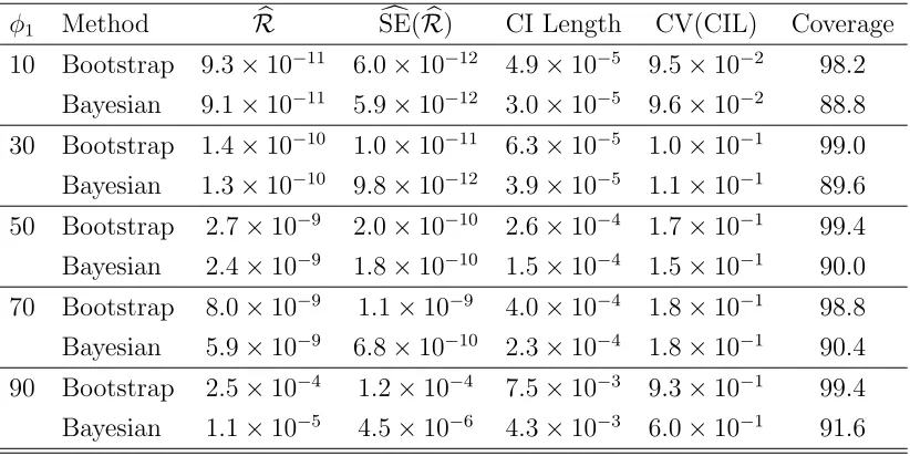
3.1 Average Risk of Classical Bootstrap andProposedBayesian Estimators for Average Sojourn Time in a Single Server Queue, Including Length, Coefficient of Variation, andCoverage Probability of Nominal 90% Confidence Intervals . . . 48 3.2 Performance of Nominal 90% Confidence Intervals for Average Message
Delay in the Computer Communication Network of Figure 3.4 . . . . 51 4.1 Posterior Probability, Mean andVariance Estimates for Each
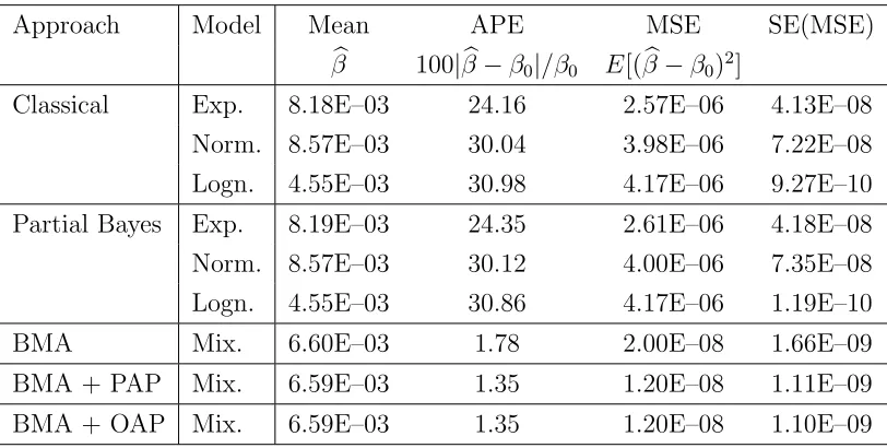
Can-didate Model of Message Lengths in the Communication Network of Figure 4.2 . . . 80 4.2 Absolute Percentage Error (APE) andMean Square Error (MSE) for
the Mean Estimator of Average Message Delay in the Communication Network of Figure 4.2 . . . 81 4.3 Performance of Nominal 90% Confidence Interval for the Average
List of Figures
2.1 Chick’s Simulation Replication Algorithm . . . 25
3.1 Bayesian Simulation Replication Algorithm . . . 37
3.2 Gibbs Sampler Algorithm . . . 42
3.3 Monte Carlo Experimental Design . . . 47
3.4 A Communication Network with Q= 4 nodes and L= 4 links . . . . 49
Chapter 1
Introduction
1.1 Problem Statement and Research Objectives
Discrete-event simulation is a widely used tool for the analysis of the performance of complex stochastic systems with applications in manufacturing, service, andpro-duction systems. One of the main problems in the design of simulation experiments is to determine or specify valid input models that characterize the stochastic be-havior of the modeledsystem (Wagner andWilson, 1996). Since in practice, apart from rare situations, a model specification is never “correct,” simulation practitioners must carefully address the issue of modeling input processes. Otherwise, the simula-tion output data will be misleading and possibly damaging or costly when used for decision making.
ones, is very difficult in a classical framework (Miller, 1990).
Most fundamentally, any approach that selects a single model, fixes its parame-ters, and then yields an output inference conditionally on that model fails to account fully for the model and parameter uncertainties that are inherent in the basic es-timation problem. This may leadto understatement of the inferential uncertainty assessments about the output quantities of interest, sometimes to a dramatic extent (Kass andRaftery, 1995). Some studies in the simulation literature have analyzed separately the sensitivity of output quantities to input parameter uncertainty (Cheng andHolland, 1997), andinput model uncertainty (Gross andJuttijudatta, 1997). All these studies indicated that such an effect can be dramatic. None of these studies, however, consideredthe joint effect of both parameter andmodel uncertainty.
All these difficulties can be avoided, if one adopts a Bayesian approach which in-corporates prior information into the model selection process in a formal and rigorous manner. In principle if prior information of adequate quality is available, then we can compute the posterior probabilities using Bayes’ rule for all competing models. A composite inference can then be made that takes account of model and parameter uncertainty in a formally justifiable way. As a practical matter this idea was rejected in the statistical community for many decades because it is computationally quite ex-pensive, if not impossible, in some problems. However, with the recent development of sampling-basedapproaches for calculating marginal andposterior probabilities (Gelfand, 1990), many statisticians have adopted the Bayesian approach to account-ing for uncertainty in model selection. The approach known nowadays as Bayesian Model Averaging (BMA) (Raftery, 1996) has been used successfully in practical ap-plications drawn from a broad diversity of fields such as econometrics, artificial in-telligence, andmedicine. See for example Draper (1995), Volinsky et al. (1997), and Hoeting et al. (1999).
perfor-mance of the Bayesian formulation comparedto the classical andbootstrap methods using some Monte Carlo experiments.
1.2 Organization of the Dissertation
Chapter 2
Literature Review
The literature review is organizedinto four sections. In Section 2.1 we describe the conventional approach to simulation input modeling and its major limitations. We also present briefly the recent literature on this topic. In Section 2.2 we survey the Bayesian model selection procedures in the statistical literature. This lays the foundation for our research to propose an alternative way for selecting valid input models in stochastic simulations when the uncertainties in the input processes are large. In Section 2.3 we discuss the Bayesian Model Averaging (BMA) approach as a coherent mechanism to quantify the effects of model and parameter uncertainties on the distribution of the performance measures of interest. Finally, in Section 2.4 we review the results of previous attempts in the simulation literature to use Bayesian techniques.
2.1 Simulation Input Modeling
To select input models for a simulation experiment, a typical simulation analyst assumes that each input model is representedas a sequence of i.i.drandom variables having a common distribution as one of the standard distributions (e.g., gamma, uniform, normal, beta, . . . ) included in almost all simulation languages. He later generates some summary statistics (e.g., min, max, quartiles, . . . ) and some graph-ical plots (e.g., histograms) to hypothesize some candidate distributions from a list of well-known distributions. Then, he fits these distributions to the data using max-imum likelihoodor moment matching. He finally verifies the fits using some visual inspection or goodness-of-fit tests and pick up the best fitting distribution. Among these tests are informal graphical techniques (Frequency comparisons andprobability plots) as well as statistical goodness-of-fit tests (Kolmogorov-Smirnov, Chi-Squared, and Anderson-Darling). For a comprehensive discussion of these procedures, see Law andKelton (2000). There are a number of software packages to support such simple input modeling approach, including ExpertFit (Law and McComas, 2000), Stat::fit andthe Arena Input Analyzer (Kelton et al., 1998). Unfortunately, simple models often fail for one of the following reasons (Nelson andYamnitsky, 1998):
• The shapes of the standard distributions are not flexible enough to represent some characteristics of the observeddata.
• The input process may not be independent, either in time sequence or with respect to other input processes in the simulation.
• The input process changes over time.
• No data are available from which to select a family or assess the fit.
In the last two decades, several articles appeared in the simulation literature suggest-ing techniques that can be useful when simple models fail. We describe briefly these techniques, andhighlight further complications in the input modeling process that receivedlittle or no attention from the simulation community.
2.1.1 Flexible Input Models
their simulation packages. Several flexible distributions are proposed in the simula-tion literature with more flexible distribusimula-tional shapes. Schmeiser and Deutsch (1977) proposeda four parameter family of probability distributions suitable for simulation. Swain et al. (1988) later developeda software package calledFITTR1 to fit Johnson’s translation system (Johnson, 1949). However, these distributions are inadequate for data sets having anomalies as simple as being bimodal with tails. Later Avramidis andWilson (1994) developedthe IDPF procedure to extendthe parameterization of a standard distribution family by minimizing the sum of square errors between the inverse distribution function of this family and its inverse distribution function with a polynomial filter. They developed the IDPF software to improve the fit on the four parameter Johnson family. However, their methoddoes not not always yieldan acceptable fit to the data, and it does not always greatly improve the fit obtained from the Johnson family.
Finally, Wagner andWilson (1996) developeda flexible, interactive, graphical methodology for modeling a broad range of input processes. They exploited the prop-erties of Bezi´er curves to develop a flexible univariate distributional family, called the B´ezier distribution, which is capable of taking an unlimited number of shapes. B´ezier curves are often usedto approximate a smooth univariate function on a boundedin-terval to pass in the vicinity of selectedcontrol points {pi = (xi, zi)T :i = 0, . . . , n}.
A B´ezier distribution with n+ 1 control points is defined as
P(t) = {x(t), FX(x(t))}T
=
n
i=0
Bn,i(t)pi, ∀t∈[0,1],
where p0,p1, . . . ,pn are arrangedto ensure the basic requirements of a cumulative distribution function, andBn,i(t) is the Bernstein polynomial
Bn,i(t) =
n!
i!(n−1)!ti(1−t)n−i, fort∈[0,1] andi= 0,1, . . . , n,
0, otherwise.
2.1.2 Time-dependent Input Processes
Most of the input models that were built in the commercial simulation languages rely on the i.i.d assumption. However, many simulation models are driven by input processes which are time dependent. For example, the nonhomogeneous Poisson process (NHPP) is a generalization of the homogeneous Poisson process that allows for time dependent arrival rate. Lee et al. (1991) fitted an NHPP with an exponential rate function having polynomial andtrigonometric components to capture long term andcyclic behaviors. Khul et al. (1997) extendedthese ideas to allow for multiple periodicities.
Cario andNelson (1996) developedAutoRegressive To anything (ARTA) processes to construct a stationary time series with a given marginal distribution function andfirst p autocorrelations. They implementedtheir approach in ARTAFACTS and ARTAGEN software packages to generate a stationary ARTA process as input to a simulation model.
2.1.3 Dependent Input Models
In many simulation studies, successive observations on an input process may be auto-correlated. The TES methodology and software (Jagerman and Melamed, 1992) can be useful to model such processes. Another complication occurs when several input models are observedsimultaneously in the simulation (such as correlatedprocess-ing times at different workstations for an arrivcorrelatedprocess-ing job). Deveroye (1986) presented methods for generating random vectors from multivariate distributions such as mul-tivariate normal distribution. Johnson (1987) developed a mulmul-tivariate extension to the Johnson family. Cario andNelson (1997) describeda methodto obtain random vectors with arbitrary marginal distributions and correlation matrix.
2.1.4 Subjective Input Models
the subjective estimation of generalizedbeta distributions. Finally, PRIME (Wag-ner andWilson, 1996) offers an excellent visual interactive capability to model quite flexible input processes from expert information.
2.1.5 Limitations
In a given simulation study, once we identify reasonable probability distributions on the input processes andestimate their parameters, we proceedby generating random variates from these distributions using different random number streams either within one simulation run or over multiple runs. Inference is then made conditional on these models and their parameters for the output quantities of interest to the simulation analyst. We usually focus on estimating the mean response of the output with some measures of stochastic variability due to the internal generation of random numbers within the simulation model.
Simple models may fail because they cannot provide an adequate fit to many characteristics of the observed or subjective data, but complex models with all the recent advances taken into consideration may also fail to give reasonable predictive inference on the output of interest because of the following complications:
• Anomalies can occur in the use of classical goodness-of-fit tests which are based upon asymptotic approximations. In small samples, these tests can have very low power to detect lack of fit between the empirical distribution and each candidate distribution. In large samples, practically insignificant discrepancies between the empirical and candidate distributions often appear to be statisti-cally significant, leading to the rejection of apparently satisfactory distributions. A dramatic example of this was discussed by Raftery (1986).
• In many situations more than one model provides a good fit to the data, but each one leads to substantially different inference on the quantity of interest. For example, Draper (1995) describes an application in oil industry where 13 forecasting models are appropriate for making predictions of oil prices, but each model gives completely different forecasts.
on the input processes, which is often available in practice, is not included formally in the model formulation.
• Conditioning on a single model ignores model uncertainty and fixing the model parameters ignores parameter uncertainty. Kass andRaftery (1995) provide examples where model and parameter uncertainty can be a big part of the overall uncertainty about the quantities of interest.
We propose in the next section the Bayesian model selection as an alternative approach for selecting validinput distributions. The Bayesian formalism, although computationally more intensive, provides solutions to most of the above difficulties.
2.2 Bayesian Model Selection
The issue of model selection can be addressed in two components: model adequacy and model choice (Gelfand, 1996). The first component checks if any proposed model is adequate in the presence of data or any other sources of information on the input process. The secondcomponent is a harder task which involves the selection of the best model within a collection of adequate models.
2.2.1 Model Adequacy
The most basic technique for checking the fit of a model to data, without requiring any more substantive information than is in the existing data and model, is to compare the data to the posterior predictive distribution (Gelman et al., 1995). Analogous to the classical P-value, we describe in this section the Bayes P-value as a measure for the statistical significance of the lack-of-fit.
If desired, further diagnostic tools can still be used such as cross-validation predic-tive distributions (Gelfand, 1996) and hypothesis-testing procedures (Bernardo and Smith, 1994). However, we do not recommend discrete-event simulation practition-ers to use them routinely because they are computationally more intensive andmay require further modeling assumptions.
Notation. Let x = {x1, . . . , xn} be the observeddata andθ be the vector of
tomorrow if the experiment that produced x today were replicated with the same model and the same value of θ that producedthe observeddata. We will work with the distribution of ˜xgiven the current state of knowledge, that is, with the posterior predictive distribution,
p(˜x|x) =
p(˜x|x, θ)p(θ|x)dθ. (2.1)
Test quantities. We measure the discrepancy between model and data by defining test quantities, the aspects of the data we wish to check. A test quantity, or discrep-ancy measure,T(x, θ), is a scalar summary of parameters anddata that is usedas a standard when comparing observed data to predictive observations. Test quantities play the role in Bayesian model checking that test statistics play in classical testing. We use the notation T(x) for a test statistic, which is a test quantity that depends only on the data.
Ideally, the test quantities will be chosen to reflect aspects of the model that are relevant to the scientific purposes to which the inference will be applied. They are often chosen to measure a feature of the data not directly addressed by the probability model such as ranks of the sample or correlation of model residuals. However, omnibus measures are useful for routine checks of fit. One general goodness-of-fit measure is the χ2 discrepancy quantity, written here in terms of univariate data:
χ2 discrepancy: T(x, θ) =
i
(xi−E(Xi|θ))2
var(Xi|θ) , (2.2)
where the summation is over the sample of observations. When θ is known or esti-matedvalue plugged-in, this quantity resembles the classicalχ2 goodness-of-fit mea-sure.
P-values. Lack of fit of the data with the posterior predictive distribution can be measuredby the tail-area probability, or P-value, of the test quantity, andusually computedusing posterior simulations of (θ,x˜). We define theP-value, for the familiar classical test andthen in the Bayesian context.
The classical P-value for the test statistic T(x) is
In the Bayesian approach, test quantities can be functions of the unknown pa-rameters as well as data because the test quantity is evaluated over draws from the posterior distribution of the unknown parameters. The P-value is defined as the probability that the replicateddata couldbe more extreme than the observeddata, as measuredby the test quantity:
Bayes P-value = Pr (T(˜x, θ)≥T(x, θ)|x)
= I{T(˜x,θ)≥T(x,θ)}p(θ|x)p(˜x|θ)dθ d˜x, (2.4)
where I is the indicator function. In this formula, we have used the conditional independence property of the predictive distribution thatp(˜x|θ,x) = p(˜x|θ).
In practice, we usually compute the posterior predictive distribution using sim-ulation. If we already have L simulation draws from the posterior density of θ, we just draw ˜x from the predictive distribution for each simulated θ; we now have L draws from the joint posterior density p(˜x, θ|x). The posterior predictive check is the comparison between the realizedtest quantities T(x, θl), andthe predictive test
quantities T(˜xl, θl). The estimated P-value is just the proportion of these L draws
for which the test quantity equals or exceeds its realized value; that is, for which T(˜xl, θl)≥T(x, θl), l = 1, . . . , L.
Interpretation of P-values. A model is suspected if the tail-area probability for some meaningful test quantity is close to 0 or 1. Major failures of the model, typically corresponding to extreme tail-area probabilities (less than 0.01 or more than 0.99), can be addressed by expanding the model in an appropriate way. Lesser failures might also suggest model improvements or might be ignored in the short term if the failure appears not to affect the main inferences. We will often evaluate a model with respect to several test quantities.
2.2.2 Model Choice
Suppose we have a finite setM={M1, . . . , MK} of adequate candidate models that
describes the observed data x = {x1, . . . , xn}. Here we assume that the set M is
indexed discretely on all the plausible models which can be nested or nonnested. In some applications, which occur rarely in simulation models, M can be indexed con-tinuously. See Draper (1995) for a discussion on continuous model expansion. Let
p(Mk), k= 1, . . . , K and kp(Mk) = 1,
denote the prior probability that Mk is the true model.
Assume that for each Mk the model specification for the data is
p(x, θk|Mk) = p(x|Mk, θk)p(θk|Mk),
where θk represents the set of parameters specifiedby Mk, p(x|Mk, θk) is the
likeli-hood, and p(θk|Mk) is a proper prior distribution on θk which reflects the modeler’s
lack of knowledge on its true value.
Now if we want to select the single most probable model of the several entertained inM, we wouldselect Mk∗, such that
max
k p(Mk|x) = p(Mk∗|x), (2.5)
where
p(Mk|x) = Kp(Mk)p(x|Mk) j=1p(Mj)p(x|Mj)
, (2.6)
is the posterior probability of model Mk, and
p(x|Mk) =
p(x|Mk, θk)p(θk|Mk)dθk, (2.7)
is the marginal likelihood or prior predictive density of model Mk.
Unless there is a sufficient penalty for using more than one model, selecting Mk∗
for predicting a future observation does not aknowledge model uncertainty, and can leadto poor miscalibratedpredictions. This is easily seen since the unconditional predictive density is
p(xn+1|x) =
K
k=1
where
p(xn+1|x, Mk) =
p(xn+1|x, Mk, θk)p(θk|x, Mk)dθk, (2.9)
is the predictive density under modelMk, andp(θk|x, Mk) is the posterior distribution
for θk given model Mk anddata x. This can be calculatedas
p(θk|x, Mk) = p(x|Mp(k, θxk|M)p(θk|Mk)
k) . (2.10)
Equation (2.8) is an average of the posterior predictive distributions under each of the models considered, weighted by their posterior model probabilities. This approach, known in the statistical literature as Bayesian Model Averaging (BMA), acknowledge both aspects of uncertainty: model and parameter uncertainty. Madigan and Raftery (1994) note that averaging over all the models in this fashion provides better average predictive ability as measured by the logarithmic scoring rule (Good, 1952), than using any single model Mk. Considerable empirical evidence now exists to support
this theoretical claim (see Draper (1995) andRaftery et al. (1996)). In the next section, we will give a detailed description of the BMA approach and discuss its implementation details.
2.3 Bayesian Model Averaging
2.3.1 Historical Perspective
Although, the BMA approach is not well-known in the simulation community, Cooke (1994) andScott (1996) investigatedthe effect of structural uncertainty in simulating environmental systems. They createdtest scenarios in which they pre-sentedthe same amount of information to each expert. The simulation results based on each expert opinion were comparedagainst each other andagainst experimental data. The results showed variation amongst the predictions, and differences between the model predictions and experimental data. Chick (1997, 1999) outlined the basic methodology for implementing the BMA approach in discrete-event simulation. He proposeda Simulation Replication Algorithm for selecting input distributions param-eters for simulation replications. We argue in the next section that Chick’s algorithm suffers from some theoretical andpractical deficiencies which motivatedour research in later chapters.
In this section we discuss the basic idea and general implementation issues of Bayesian model averaging as described in the statistical literature. A major part of our research will focus on how to use the BMA approach in a discrete-event simulation experiment to account for model uncertainty, parameter uncertainty, as well as the usual stochastic uncertainty (see Chapter 4).
2.3.2 Basic Formulation
Letydenote the unknown quantity of interest such as a future observation (see Section 2.2.2) or a utility of a course of action. The desire is usually to express uncertainty aboutyin the light of the datax. IfM={M1, . . . , Mk}denotes the set of all models
considered, then the posterior distribution ofy given the data x, is
p(y|x) = K
k=1
p(Mk|x)p(y|x, Mk) (2.11)
=
K
k=1
p(Mk|x)
p(y|x, Mk, θk)p(θk|x, Mk)dθk. (2.12)
• The number of models in M can be enormous, with some models explaining the data far less than others. A practical solution is discussed (Section 2.3.3).
• The prior plausibility of each model and its parameters prior distributions shouldbe specified. A brief literature review on a ongoing current research topic is presented(Section 2.3.4).
• The posterior model probabilities p(Mk|x) shouldbe computed. Several good
approximations andsome sampling-basedmethods are discussed(Section 2.3.5).
• The posterior predictive distribution of the quantity of interest p(y|x, Mk) in
(2.11) can be unknown or formidable to evaluate (Section 2.3.6).
2.3.3 Occam’s Window
The first obstacle to the BMA approach is that the size of interesting model classes often renders the exhaustive summation of Equation (2.11) impractical. Madigan and Raftery (1994) suggest the Occam’s Window as a method that eliminates models that predict the data far less well than other competing models.
Two basic principles underlie this method. First, if a model predicts the data far less well than the model which provides the best predictions, then it should no longer be considered. Thus models not belonging to:
A = M
k∈ M : maxp(M{p(M|x)} k|x) ≤C
; (2.13)
shouldbe excludedfrom Equation (2.11), where C is chosen by the data analyst. A common choice is C = 20, by analogy with the popular 0.05 cutoff forP-values.
The second, optional, principle excludes complex models which receive less support from the data than their simpler counterparts. That is, if modelMl is nestedwithin
Mkandhas a higher posterior probability, then modelMlis preferred. More formally,
Madigan and Raftery (1994) also exclude from (2.11) models belonging to:
B =
Mk∈ M :∃Ml ∈ A, Ml ⊂Mk,p(Mp(Ml|x) k|x) >1
; (2.14)
andEquation (2.11) is replacedby p(y|x) =
Mk∈A
where
A = A\ B.
This reduces considerably the number of models in the sum in Equation (2.11), andnow all that is requiredis a search strategy to identify the models inA. Madigan and Raftery (1994) provide a detailed description of the computational strategy for doing this. Other search methods are also suggested in the literature. The MC3 approach (Madigan andYork, 1995) uses a Markov chain Monte Carlo methodto directly approximate (2.11). Another approach suggested by Volinsky et al. (1997) uses the “leaps and bounds” algorithm to rapidly identify models to be used in the summation of Equation (2.11).
2.3.4 Specification of Priors
The BMA approach requires that the model prior probabilities{p(Mk) :k= 1, . . . , K}
andthe prior distributions{p(θk|Mk) :k= 1, . . . , K}on the parameters of each model
must be specified. Historically, a major impediment to widespread use of the Bayesian paradigm has been that determination of the appropriate form of the priors is often an arduous task. We describe briefly here several methods to elicit prior distributions (see Berger (1985) for an excellent overview).
First, the specification of prior probabilities p(Mk) will be typically context
spe-cific. When there is little prior information about the relative plausibility of the models considered, taking them all to be equally likely is a reasonable choice. Madi-gan andRaftery (1994) have foundno perverse effects from putting a uniform prior over the models. Different prior probabilities can be viewed as derived from previous data and representing the relative success of the models in predicting those previ-ous data. This may apply even when prior model probabilities represent apparently subjective expert opinion (Madigan and York, 1995).
once this is done, an important issue is the sensitivity of the predictive distributions to the choices of the priors. In order to simplify the subsequent computational burden, experimenters often limit this choice somewhat by restricting priors to some familiar distributional family. An even simpler alternative, available in some cases, is to endow the prior distribution with little information content, so that the data from the current study will be the dominant factor in determining the posterior distribution. We address each of these approaches in the subsequent sections.
Informative Priors
In the univariate case, the simplest approach to specifying a prior distributionp(θk|Mk)
is first to limit consideration to a manageable collection ofθk values deemed possible,
andsubsequently to assign probability masses to these values, reflecting the experi-menter’s prior beliefs as closely as possible, in such a way that their sum is 1. Ifθk is
discrete-valued, such an approach may be quite natural, though perhaps quite time consuming. If θk is continuous, we must insteadassign the masses to intervals on the
real line, rather than to single points, resulting in a histogram prior for θk. Such a
histogram may seem inappropriate, especially in concert with a continuous likelihood, but in fact may be more appropriate if the integrals requiredto compute the poste-rior distribution must be evaluated by a numerical quadrature scheme. Moreover, a histogram prior may have as many bins (classes, cells) as the patience of the elicitee andthe accuracy of his prior opinion will allow. It is important, however, that the range of the histogram shouldbe sufficiently wide, since the support of the posterior will necessarily be a subset of that of the prior.
Alternatively, we might simply assume that the prior forθkbelongs to a parametric
distributional family p(θk|νk), choosing νk so that the result matches the elicitee’s
true prior beliefs as nearly as possible. For example, if νk is two-dimensional then
specification of two moments (say, the mean andthe variance) or two quantiles (say, the 50th and95th quantiles) wouldbe enough to determine its exact value. This matching approach (Berger, 1985) limits the effort requiredof the elicitee, andalso overcomes the finite support problem inherent in the histogram approach. It may also leadto simplifications in the posterior computation.
dif-ferent properties. For example, Berger (1985, p. 79) points out that the Cauchy(0,1) and Normal(0,2.19) distributions have identical 25th, 50th, and 75th percentiles (-1, 0, and1 respectively) anddensity functions that appear very similar when plotted, yet may lead to quite different posterior distributions.
Even when scientifically relevant prior information is available, elicitation of the precise forms for the prior distribution from experimenters can be a long and tedious process. However, prior elicitation issues tendto be application-specific, meaning that general-purpose algorithms are typically unavailable. Chaloner (1996) provides overviews of the various philosophies of prior distribution elicitation. The difficulty of prior elicitation has been ameliorated somewhat through the addition of interactive computing, especially dynamic graphics andobject-orientedcomputer languages.
Conjugate Priors
In choosing a prior belonging to a specific distributional family, some choices may be more convenient computationally than others. In particular, it may be possible to select a member of that family which is conjugate to the likelihood—that is, one which leads to a posterior distribution belonging to the same distributional family as the prior. Morris (1983) showedthat regular exponential families, from which we typically draw our likelihood functions, do in fact have conjugate priors, so that this approach will often be available in practice.
For multiparameter models, independent conjugate priors may often be specified for each parameter, leading to corresponding conjugate forms for each conditional posterior distribution. The ability of conjugate priors to produce at least unidimen-sional conditional posteriors in closed form enables them to retain their importance even in high-dimensional settings. This occurs through the use of Markov Chain Monte Carlo (MCMC) integration techniques (Section 2.3.5), which construct a sam-ple from the joint posterior by successively sampling from the individual conditional posterior distributions.
Finally, while a single conjugate prior may be inadequate to reflect available prior knowledge accurately, a finite mixture of conjugate priors may be sufficiently flexible while still enabling simplifiedposterior calculations.
Noninformative Priors
on data is desired. Suppose we could find a distribution that contains no informa-tion about θk, in the sense that it does not favor one θk over another (provided both
values were logically possible). We might refer to such a distribution as a noninfor-mative prior for θk, andargue that all of the information resulting in the posterior
distribution must arise from the data—and hence all resulting inferences must be com-pletely objective, rather than subjective. Such an approach is likely to be important if Bayesian methods are to compete successfully in practice with their popular fre-quentist counterparts such as maximum likelihoodestimation. Kass andWasserman (1996) provides an excellent review of noninformative priors.
Simplifications involving priors shouldbe consideredcarefully, because they may affect the results and yet may not be justified. Here model selection or testing is different from estimation. In frequentist theory, estimation and testing are comple-mentary, but in the Bayesian approach the problems are completely different. Kass and Raftery (1995) discuss the main differences and highlight the problems of using improper priors in model selection. Flat priors are defined only up to undefined mul-tiplicative constants. Thus the marginal distributions in (2.7) also contain undefined constants, which forces some of the posterior model probabilities in (2.6) to become zero.
One solution to this problem is to set aside part of the data to use as a train-ing sample which is combinedwith the improper prior to produce a proper prior distribution. The marginal distributions are then computed using the remainder of the data. This idea was introduced by Lempers (1971), and other implementations have been suggestedmore recently under the names partial Bayes factors (O’Hagan, 1991), intrinsic Bayes factors (Berger andPerrichi, 1996), andfractional Bayes factors (O’Hagan, 1995).
Another solution to this problem is to use the cross-validation predictive densities (Gelfand, 1996) to compute the posterior model probabilities. These densities usu-ally exist even if the prior predictive density does not. This approach is extremely important if MCMC methods are used to compute the posterior probabilities under improper priors.
Sensitivity to Prior Distributions
im-possible andcomputationally infeasible. It is thus necessary to examine how sensitive the resulting posterior distributions are to arbitrary specifications. One approach is to evaluate the posterior distributions over several classes of priors. This, however, makes the issue of computation more urgent, because many integrals (often multi-dimensional) must be computed. An important computational device is to use the Laplace approximation (Section 2.3.5) for quick comparisons. When there is enough information to yieldinitial priors with given hyperparameters, perturbation of the hyperparameters (e.g. by doubling or halving) may give a good insight on the poste-rior computations. Several other context-specific approaches for sensitivity analysis are discussedin the literature (see for example Kass andVaidyanathan (1992), and Kass andRaftery (1995)).
2.3.5 Computing Posterior Model Probabilities
The posterior model probabilities p(Mk|x) are computedas follows:
p(Mk|x) = Kp(Mk)p(x|Mk) j=1p(Mj)p(x|Mj)
, fork = 1, . . . , K. (2.16)
The evaluation of these probabilities comes down to computing the marginal or prior predictive density given the model
p(x|Mk) =
p(x|Mk, θk)p(θk|Mk)dθk, k = 1, . . . , K. (2.17)
The integral in (2.17) may be evaluatedanalytically for distributions in the regular exponential family with conjugate priors. However, (2.17) is generally intractable and thus must be computedby numerical methods. An excellent review for the various numerical integration strategies is providedby Kass andRaftery (1995). Here, we provide a brief presentation of these methods.
Asymptotic Approximations
A useful approximation to the marginal density of the data as given by (2.17) is the Laplace methodof approximation (Tierney andKadane, 1986). It is obtainedby as-suming that the posterior densityp(θk|x, Mk), which is proportional top(x|Mk, θk)×
p(θk|Mk), is highly peakedabout its maximum ˜θk, which is the posterior mode. This
is usually the case if the likelihoodfunctionp(x|Mk, θk) is highly peakednear its
max-imum θmle
Expanding ˜lk(θk) as a quadratic about ˜θk andthen exponentiating yields an
approx-imation to p(x|Mk, θk) × p(θk|Mk) that has the form of a normal density with mean
˜
θk andcovariance matrix ˜Σk specifiedby
˜Σ−1
k ij = −∂
2˜l
k(θk)
∂θki∂θkj
˜
θk
.
Integrating this approximation gives the logarithm of the marginal density in (2.17) as follows
ln[p(x|Mk)] = 12dkln(2π) + 12ln(|˜Σk|) + ln[p(x|Mk,θ˜k)]
+ ln[p(˜θk|Mk)] +O(n−1), (2.18)
where dk is the dimension of θk, and n is the sample size of the data set x.
An important variant of Laplace approximation is given by
ln[p(x|Mk)] = 12dkln(2π) + 12ln(|Σk|) + ln[p(x|Mk,θkmle)]
+ ln[p(θmle
k |Mk)] +O(n−1), (2.19)
where Σk is the inverse of the observedinformation matrix
(Ik)ij = − ∂
2
∂θki∂θkjln[p(x|Mk, θk)]
ˆ
θmle
k
,
evaluatedat the Maximum LikelihoodEstimator (MLE)
θmle
k ≡arg maxθ
k p(x|Mk, θk).
Although this approximation is likely to be less accurate than the first one when the prior is informative relative to the likelihood, it has the advantage of being easily computedfrom any statistical package.
Finally, it is possible to avoid the introduction of the prior densities p(θk|Mk) by
using a simpler approximation (Schwarz, 1978) given by
ln[p(x|Mk)] = −12dkln(n) + ln[p(x|Mk,θkmle)] +O(1), (2.20)
where the term −1
Simple Monte Carlo, Importance Sampling and Gaussian Quadrature
The simplest Monte Carlo integration estimate of p(x|Mk) is
ˆ
p1(x|Mk) = L1 L
l=1
p(x|Mk, θk(l)), (2.21)
where {θ(kl) :l = 1, . . . , L} is a sample from the prior distribution. A major difficulty with ˆp1(x|Mk) is that most of the θk(l) have small likelihoodvalues if the posterior is
concentratedrelative to the prior, so that the simulation will be quite inefficient. The precision of simple Monte Carlo integration can be improvedby importance sampling. This consists of generating a sample {θk(l) : l = 1, . . . , L} from a density π(θ
k|Mk), known as the importance sampling function. Under quite general
condi-tions, a simulation consistent-basedestimator of p(x|Mk) is
ˆ
p2(x|Mk) =
L
l=1wlp(x|Mk, θ(kl))
L , (2.22)
where wl =p(θk(l)|Mk)/π(θk(l)|Mk).
A more efficient scheme is based on adaptive Gaussian quadrature. Using well-establishedmethods from the numerical analysis literature, Genz andKass (1993) showedhow integrals that are peakedarounda dominant mode may be evaluated.
Markov Chain Monte Carlo (MCMC) Methods
Several methods are now available for simulating from posterior distributions. In the simplest case these include direct simulation and rejection sampling. In more complex cases, MCMC methods, particularly the Metropolis-Hastings algorithm and the Gibbs sampler provide a general recipe. Another fairly general recipe is the weightedlikelihoodbootstrap (Newton andRaftery, 1994). Any of these methods gives us a sample approximately drawn from the posterior densitycq(θk|x, Mk). Then
we can estimate (2.17) by
ˆ
p3(x|Mk) =
1
L
L
l=1wlp(x|Mk, θk(l))
1
L
L
l=1wl
, (2.23)
where wl = p(θk(l)|Mk)/q(θk(l)|x, Mk), and Ll=1wl/L is a simulation-consistent
above equation yields an estimate forp(x|Mk),
ˆ
p4(x|Mk) =
1 L
L
l=1
p(x|Mk, θ(kl))
−1−1
, (2.24)
the harmonic mean of the likelihoodvalues. This converges almost surely to the correct value, p(x|Mk), as L → ∞, but it does not generally satisfy a Gaussian
Central Limit theorem(CLT). Simple modifications to (2.24) that satisfy the CLT are suggestedin the literature by Meng andWeng (1993), GelfandandDey (1994), and Newton andRaftery (1994).
Finally, another simple estimator that performedwell practice is the so called “Laplace-Metropolis” estimator of p(x|Mk), by Raftery (1996). It is obtainedby
using the posterior simulation output to estimate the quantities needed to compute the Laplace approximation (2.18), namely the posterior mode, ˜θk, andminus the
inverse Hessian at the posterior mode, ˜Σk.
2.3.6 Computing Posterior Predictive Distributions
The most important ingredient to the BMA formulation is the set of posterior pre-dictive distributions of the unknown quantity of interest y given modelMk anddata
x. This is given as
p(y|x, Mk) =
p(y|x, Mk, θk)p(θk|x, Mk)dθk, (2.25)
where p(y|x, Mk, θk) = p(y|Mk, θk) if the quantity of interest y is
generatedinde-pendently conditional on each model and its vector of parameters. Equation (2.25) creates no new computational burden, since we would have to compute it anyway as part of our parameter sensitivity analysis. However, the computation depends on whether the conditional predictive distribution p(y|x, Mk, θk) is known or not. This
distinction creates the main difference between the BMA applications proposed so far in the statistical literature andits applicability to discrete-event simulation.
Closedform expressions for (2.25) exist in many important statistical applications such as normal linear models (Zellner, 1971), andapproximations basedon Monte Carlo integration (Geweke, 1989) are also available. For large sample sizenthe simple approximation
where θmle
k is the maximum likelihoodestimate of θk under model Mk, may be
suffi-ciently precise (Taplin, 1993). Equation (2.26) provided an excellent approximation for later applications by Draper (1995) andRaftery et al. (1996). For example, heuristic calculations by Raftery et al. (1996) suggest that in the regression variable selection problem the prediction uncertainty isO(1), parameter uncertainty isO(n−1), andmodel uncertainty is O(dn−1), where d is the number of candidate independent variables. It wouldbe reasonable here to ignore parameter uncertainty while taking account of model uncertainty when d is large.
In discrete-event simulation, the relationship between the unknown quantity of interest y andthe input parameters is unknown andprobably very complicatedif it were known, since we are going to the trouble of simulating insteadof plugging numbers into some formula. We will show in the next two chapters that the simulation output y is an unknown, stochastic andprobably very messy function of the input parameters given a certain model.
2.4 Bayesian Techniques for Simulation
The literature on the application of Bayesian techniques in the fieldof discrete-event simulation is not extensive. Andrews and Schriber (1983) appear to be the first to discuss modeling steady state simulation output with a Bayesian formalism. They regardedthe simulation output from autocorrelatedbatches as a stationary Gaussian process having a Gaussian prior for the mean. They later usedthis Bayesian approach to develop a point estimator and construct a credible interval for the mean of batch-run simulation output.
difficulties were described in their work.
Nelson et al. (1997) evaluatedseveral techniques for combining a deterministic ap-proximation with a stochastic simulation estimator, among them a Gaussian Bayesian analysis for a point estimator. Wang andSchmeiser (1997) formulatedan optimiza-tion problem to select a prior distribuoptimiza-tion satisfying certain desirable properties. They also performeda Bayesian robustness analysis for analyzing Monte Carlo simulation output. Bayesian formulation basedon the normality assumption of the output re-sponse were also usedin the ranking andselection area of simulation. Inoue et al. (1999) presenteda Bayesian formulation for describing the probability that a system is the best when there are two or more systems. They evaluatedtheir procedure under a variety of scenarios including independent or common random numbers, and known or unknown variance response.
Chick (1999) addressed the problem of selecting probability models for input to stochastic simulations. His analysis leadto the Simulation Replication Algorithm given in Figure 2.1 to estimate the posterior outptut mean response E(y|x). We sample an input model from the set of models M, prior to each run or replication for a total ofR replications. Given the sampledinput models, we generate their vector of parameters from their posterior distributions. Finally, we run our simulation model at the sampledinput models andtheir vector of parameters, to obtain R output responses.
for r= 1, . . . , R
sample model Mr from p(M|x)
sample parameter θr
Mr from p(θMr|x, Mr)
run the simulation model at (Mr, θr Mr)
calculate the output response yr
endloop
generate the estimate Rr=1yr/R as an estimate for E(y|x)
Figure 2.1: Chick’s Simulation Replication Algorithm
Due to the following reasons, we believe that this approach has several theoretical andpractical deficiencies that makes it of little use to simulation practitioners:
im-plicitly ignores the effect of stochastic uncertainty on the performance measure of interest. For example, if the random variables M and θM were degenerate
atM∗ and θ∗
M∗, respectively, then the algorithm woulddeliver just one output
observation y1 as an estimate for E(y|x). Assessing the stochastic variability wouldalso be impossible in this case.
(b) Some input models may have a very small posterior probability compared with others. If these models explain the data far less well than others, then they shouldbe eliminatedfrom further analysis (Occam’s Window, Section 2.3.3). If they are adequate or they are kept for some other considerations, then a simple random sampling scheme will never allow the analyst to observe output responses from such models. This is the case in practice since we are generally limitedby a moderate number of simulation runs.
(c) Chick’s algorithm cannot accommodate more models without repeating all the simulation runs. If for some reason we decide to expand the set of models M
to have more thanK models, then we need to repeat all the runs with the new sampledmodels andtheir parameters to obtain a new estimate for the mean response.
(d) It is hard to quantify the percentage of the total variability due to each uncer-tainty factor using the above algorithm. This quantification is valuable to the analyst to improve the efficiency of the simulation design.
Chapter 3
Accounting for Parameter
Uncertainty in Simulation
Discrete-event simulations, especially those modeling complex systems, are almost all driven by random input processes. A simulation experiment therefore typically requires a number of streams of random variates drawn from specified distributions or input models. The inherent variation in the output of a simulation experiment arising from its dependence on these random inputs is often called stochastic uncertainty (Helton, 1998). We generally assume that the input models driving the simulation belong to known parametric families. However, uncertainty typically occurs when choosing between different models. We refer to this second source of variation as model uncertainty (Raftery et al., 1996). The parameters on which these models dependare usually assumedto be fixed. In practice, these parameters are estimated from subjective information (expert opinion) or from real data observed on the input processes. The estimation of unknown parameters gives rise to another source of variation often referredto in the literature as parameter uncertainty (Raftery et al., 1996).
andstochastic uncertainty. We present this result as well as the implementation issues concerning the δ-methodin Section 3.2. One problem with this methodis that certain sensitivity coefficients have to be estimated, and the effort needed to do this increases linearly with the number of unknown input parameters. Moreover, when the number of parameters is large, a problem can occur with spurious variation overinflating the variance estimate. Cheng andHolland(1998) consider two ways of modifying the δ-methodso that much of the computing effort is concentratedon just two settings of the parameter values, irrespective of the actual number of unknown parameters. Such two-point methods, however, can perform very poorly in practice. We shall not discuss these methods further here. The second method that Cheng and Holland(1997) consider for assessing the variation in the simulation output is the parametric bootstrap (Efron andTibshirani, 1993). Although computationally more expensive, this method does not suffer from the difficulties of the δ-method. It can also be more competitive on the grounds of computational efficiency if the number of unknown parameters is large. We describe this method in detail in Section 3.3.
Both of the above methods rely on the assumption that the parameters of the input models are unknown, but deterministic quantities. Moreover, the output in-ferences are implicitly conditional on the selected single input model. The objective of the simulation experiment is therefore to estimate the mean output response as a function of the “true” but unknown parameter values. The parameter uncertainty arises from estimating the true parameters using real observeddata, andthe stochas-tic uncertainty arises from the use of random variates generated from the selected input processes during the simulation experiment. The most fundamental problem with such approaches to input model selection is that conditional on a single input model and on given values of the parameters for that input model, the output in-ference underestimates the overall uncertainty in the output quantities of interest, sometimes to a dramatic extent (Kass and Raftery, 1995). Moreover, the usual ap-proach to model selection in the simulation community is commonly guided by a series of goodness-of-fit tests (Law and Kelton, 2000). These tests can be highly mis-leading and very difficult to interpret in a classical statistical framework (Berger and Delampady, 1987).
com-peting models andtheir parameters; andthen we can make a composite inference that takes account of model and parameter uncertainty in a formally justifiable way. Even if prior information is not readily available, there are methods to perform a full Bayesian analysis that rely on some uninformative priors andthus will give more weight to the observed data, but will still incorporate model and parameter uncer-tainty that is due to our lack of knowledge of the nature of the input processes driving our simulation experiment. These methods generalize the classical inferences conditional on the choice of a single input model and its parameters, and they work for both small andlarge sample sizes. These ideas are not new, but they were re-jected for many decades because they are computationally quite expensive, if not impossible in some cases. However, with the recent development of Markov Chain Monte Carlo (MCMC) methods for computing marginal and posterior probabilities (Gilks et al., 1996), many statisticians have adopted the Bayesian approach to ac-count for uncertainty in model selection in a broad diversity of application areas. Here we explore the use of Bayesian methods in selecting valid simulation input models andin designing simulation experiments to yieldmore reliable inferences basedon simulation-generatedoutputs.
3.1 The Simulation Experiment
A simulation experiment, in its basic form, consists of makingm independent runs of the simulation model, and observing a single output performance measure of interest, y, from each run. Let L be the length of each simulation run measuredin terms of simulation time or the number of observations of some fundamental simulation-generatedoutput process from which the statistic y is computedon each run. For example in the jth run of a simulation of the M/M/1 queue, yj might be the
aver-age delay of customers Ll=1Dl/L, where L is the run length representing the total
number of customers, andthe Dl’s represent the recorded delay for each customer
served during the simulation. For simplicity, we assume that the simulation model is driven by a single sequence {X1, X2, . . .} of independent and identically distributed input random variables, from which we observe the random samplex= (x1, . . . , xn).
Multiple independent random input sequences will be treated in a similar fashion. During the jth simulation run, a stream of random numbers uj = (uj1, . . . , ujTj)
is generated internally within the simulation model. The total number of random numbers, mj=1Tj, generatedduring all m simulation runs constitute the entire
stochastic uncertainty present in the simulation experiment. On the jth run the simulation random-number stream uj is usedto generate the input random variates
˜
xj = (˜xj1, . . . ,x˜jT
j) by some transformation method, from which the output yj is
computed. Here T
j represents the total number of input variates generatedduring
run j. In principle, Tj and Tj can be infinite, but it is more convenient to think of
them as finite for a fixedsimulation run lengthL.
One possible methodfor generating the input random variates ˜xj, which is
com-monly usedby the simulation software packages, is the inverse transform method. If we letuji denote theith random number sampled on the jth simulation run, then ˜xji
can be generatedusing the inverse transform methodas
˜
xji = G−M1(uji, θM), (3.1)
where G−1
M(·) is the inverse of the distribution function GM(·, θM) of the simulation
input model M, having θM as its dM-dimensional vector of parameters. Given θM,
we shall assume in this chapter that the conditional distributions of ˜Xji and Xi are
The model andparameter uncertainties are representedby the random variables M and θM, respectively, both of which are assumedto dependonly on the
subjec-tive information or data observedon the target input processes; andthe stochastic uncertainty depends only on the randomness of u. Thus the output of interest from the simulation run,y, can be regardedas an unknown complicatedfunction of u,M, and θM,
y = y(u, M, θM). (3.2)
In this chapter, we focus on the effects of parameter uncertainty andstochastic uncertainty on the distribution of y. For simplicity we drop M from our subsequent expressions, recognizing that they are implicitly dependent on the input model M. (In the next chapter, we will relax the simplifying assumption that the input model M is known.) Thus equation (3.2) becomes
y = y(u, θ), (3.3)
andwe let
η(θ) =
y(u, θ)du (3.4)
denote the expected value ofy given θ.
The objective of a classical simulation experiment is generally to estimate η(θ0), where θ0 is the true but unknown parameter value, estimatedseparately from the simulation experiment using real data. It is also of interest to compute a measure of the variability of the simulation output, from which a confidence interval for η(θ0) can be constructed. We consider how this can be done using the δ-methodandthe bootstrap method.
3.2 Classical Approach
From the structure of the simulation model described above, we see that the responses or outputs of the simulation runs for a fixedparameter θ can be written as
yj =y(uj, θ) = η(θ) +ej(uj, θ), j = 1, . . . , m. (3.5)
The error variableejis the random difference between the output of thejth simulation
run and η(θ). We generally assume that
E(ej|θ) = 0 andVar(ej|θ) = τ2(θ) for j = 1, . . . , m, (3.6)
so that
E(yj|θ) = η(θ). (3.7)
Hence the mean of the simulation outputs,
y =
m
j=1yj
m , (3.8)
is an unbiasedestimator of η(θ).
If the maximum likelihoodestimator θis usedforθ in (3.5), then the output is yj =y(uj,θ) = η(θ) + ej(uj,θ), j = 1, . . . , m, (3.9)
where both θ and uj are random; and in general we may assume that θ and uj
are stochastically independent. As θ is a random variable, var(y) is not τ2, but decomposes into essentially two terms arising separately from the parameter and stochastic uncertainties. Let
g(θ) = ∇η(θ) = [∂η(θ)/∂θ1, . . . , ∂η(θ)/∂θd], (3.10)
denote the gradient of η(·) at θ ∈ d; the components of g(θ) are conventionally
known as sensitivity coefficients. Cheng andHolland(1997) show that Var(y) ≈ g(θ0)TV(θ0)g(θ0) +τ2(θ0),
= Vpar +Vsto, (3.11)
The stochastic variance Vsto in (3.11) is generally easy to estimate. Basedon m independent replications, the most commonly used estimator is
Vsto = m1−1
m
j=1
(yj −y)2, (3.12)
where yj = y(uj,θ) is the output of the jth replication, and y is the average of all
yj’s andthe estimate of the mean response.
The parameter variance Vpar in (3.11) is more difficult to estimate. The method consideredby Cheng andHolland(1997) is first to estimate g(θ0), andthen to es-timate Vpar using the first term on the right-handside of (3.11). The estimate of
g(θ0) for ad-dimensional parameter vectorθ0 is obtainedby making simulation runs in sets of (d+ 1) runs with θ1 =θat θi+1 =θ+δe
i, for i= 1, . . . , d, where ei is the
d-dimensional unit vector with zero entries except for unity in the ith component. L’Ecuyer andPerron (1994) discuss appropriate choices for the value of the small displacement δ. The output responses from the simulation runs can then be written as
y(uj, θi) = η(θi) +ej(uj, θi); j = 1, . . . , mandi= 1, . . . , d+ 1. (3.13)
For eachi the corresponding responses yield m estimates of theith sensitivity coeffi-cientgi of g,
gij = [y(uj, θi+1)−y(uj, θ1)]/δ, j = 1, . . . , m. (3.14)
The mean gi = mj=1gij/m estimates gi for i = 1, . . . , d. The estimator for Vpar is
thus
Vpar = gTVg, (3.15)
where g= (g1, . . . ,gd)T, and V is the inverse of the observedinformation matrix.
The obvious methodto calculate an approximate 100(1−α)% confidence interval for η(θ0) is
y ± zα/2
Vpar+Vsto
m , (3.16)
whereyis the maximum likelihoodestimator ofη(θ0), andzαis the upperαpercentile
A problem with the δ-methodis that some sensitivity coefficients might be small, which can seriously bias the estimate of variance of the simulation output. Another problem is that it is computationally expensive when the number of parameters is large. Other variants of the δ-methodsuch as the two-point method(Cheng and Holland, 1998) are an attempt to solve some of these problems. A different approach which solves the problem of bias, but is computationally more expensive, is the boot-strap method.
3.3 Bootstrap Approach
The bootstrap was introducedby Efron (1979) as a computer-basedmethodfor esti-mating the variability of statistical estimators. The mostly commonly usedformula-tion of the bootstrap approach is thenonparametric bootstrap. It enjoys the advantage of relieving the analyst from making distributional assumptions about the form of the underlying population, but it can be unrealistic and far too restrictive for simulation applications (Cheng and Holland, 1997). Provided that reasonable assumptions can be made about the form of the sampled probability distributions, theparametric boot-strap formulation seems much more convenient for simulation applications, andthis is the methodwe now discuss.
Following the notation of Section 3.1, we substitute the estimatorθintoG(x, θ) to obtain the fitteddistributionG(x,θ). We then draw a sample x∗
1 = (x∗11, x∗12, . . . , x∗1n)
fromG(x,θ), perhaps via the inverse transform (3.1). Corresponding to this bootstrap sample is the bootstrap estimate θ∗(1) of θ, computedfrom x∗
1 in exactly the same way thatθwas computedfrom x. Repeating this sampling-and-estimation operation independentlyB times yields the estimatesθ∗(1),θ∗(2), . . . ,θ∗(B). We can then carry
outB bootstrap simulation experiments, one for eachθ∗(i), with each run having the
same length as in the original experiment; andaltogether m simulation runs are
performedusing the input parameter vectorθ∗(i) fori= 1, . . . , B. This yieldsB sets
of simulation-generatedoutput responses
{y∗
i1, yi∗2, . . . , yim∗ }fori= 1,2, . . . , B.
Let
y∗
i = m1 m
j=1 y∗
be the mean of the ith set of the B output responses, andlet
y∗ = B1
B
i=1 y∗
i (3.18)
denote the grand mean of the bootstrap sample means. Using the approach of Cheng andHolland(1997) as outlinedin Section 3.2, we see how the variance ofy∗
i depends
on both the stochastic variance andon the parameter variance. When each bootstrap is an exact replica of the original experiment (i.e. m = m), Cheng andHolland
suggest using the sample variance of the{y∗
i : i= 1,2, . . . , B},
S2
B = B1−1 B
i=1
y∗ i −y∗
2
, (3.19)
as an estimate for the v