ABSTRACT
CAO, YINGFANG. Bayesian Based Structural Health Management and Reliability Analysis Techniques Utilizing Support Vector Machine. (Under the direction of Professor Mohammad N. Noori.)
Structural health and safety play a major role in all facets of human daily lives. Over the past few
decades significant advancements have been made in structural damage detection and health
management in a wide range of engineering disciplines and practices, including but not limited to
aerospace, power generating plants, infrastructure systems, and manufacturing. Two main thrust
areas of research in this field include the development of methodologies/algorithms for detection of
damage and/or changes in the dynamic characteristics of the system, and the sensing/detection
devices for capturing the required data/information. A third and evolving area is the integration of
these two thrusts and the development of integrated systems that can “manage”, and “adapt” in an
“intelligent” sense, the subsequent actions that need to take place in order to maintain the integrity of
the system subject to the external environment and/or loading conditions. However, majority of the developed techniques fail to take into account the important effects of uncertainty presented in
sensing, system modeling, and material behavior associated with dynamic systems. These
uncertainties could greatly affect the structural performance and health management, which leads to
challenging issues such as reliability and life prediction of the structure. In order to address these
important factors, the application of the probabilistic and reliability analysis techniques to structural
health management has emerged as an active research area in recent years.
Bayesian probabilistic analysis is such a technique in which the uncertainties could be related with a
mathematical model -- probability distribution function- which interprets the measurement of
confidence interval. The posterior probability distribution is known as an expression for the statistical
knowledge of a system after a set of measurements is made. The Bayesian approach is a powerful
way to continuously optimize the “posterior” probably density function (pdf) by adapting the
to be possible to perform statistical based system identification, structural damage detection and
reliability assessment, as part of structural health management.
In the first stage of this thesis work, a Bayesian based system identification approach was developed
to identify system parameters provided so that inherent uncertainties and probabilities of system
changes and/or environmental disturbances are taken into account. It is obvious that the nature of
changes encountered the system models is critical to monitoring and managing the integrity of the
structural systems. In this part of the work, system changes were modeled as random variables with
certain statistical properties. The effects of priori definition and different data sampling techniques
were studied. To explore the application of this Bayesian based system identification approach to
structural health management, the probability density function (pdf) profiles of model parameters
were studied to quantify the uncertainties associated with the estimated parameters. By analyzing the
posterior pdf inference, the reliability parameters of interest could also be obtained from the available
data.
Structural health monitoring, damage detection and structural reliability are usually considered as the
sequential components in a structural health management chain. It is the ultimate goal of structural
health management to achieve a significant improvement of the structural reliability. Therefore, the
second stage of this thesis work was devoted to the study of system reliability. A reliability analysis
package developed in MATLAB – PROBES was enhanced with its functionality in this work. The
enhancements include the new capabilities of performing analysis to correlated, non-normally
distributed random variables and the added functionality to obtain the statistical information for
system performance function. However, it was noticed that due to the lack of a complete
understanding and predicting the structural response under various environmental impacts, changes
and variations occurring in a structure through its life time, and/or modifications and redesign of a
Bayesian based uncertainty analysis technique was introduced to give statistical information of failure
probability. By utilizing the capability of Bayesian analysis to combine prior knowledge with the
subjective information, the probability properties of system reliability could be optimized
continuously. The probability test was performed to give statistical information of the current state
reliability information.
In the last stage of this work, a Bayesian based approach combined with Support Vector Machine
(SVM) was introduced to develop a novel technique of reliability analysis. Support Vector Machine
is a learning algorithm for classification and regression. A unique characteristic of this method is its
ability to provide good performance with small size of data sets. The failure probability obtained
with this newly developed technique was compared to traditional reliability analysis methods
including Monte Carlo simulation method, first order reliability method and second order reliability
method. It was demonstrated that this SVM based approach leads to a more accurate and efficient
reliability analysis algorithm. Effect of different kernel functions were investigated and compared for
both linear and nonlinear cases. It is proved that utilization of SVM is a promising area for structural
BAYESIAN BASED STRUCTURAL HEALTH MANAGEMENT AND RELIABILITY ANALYSIS TECHNIQUES UTILIZING SUPPORT VECTOR
MACHINE
By
YINGFANG CAO
A dissertation submitted to the Graduate Faculty of North Carolina State University
In partial fulfillment of the Requirements for the degree of
Doctor of Philosophy
MECHANICAL ENGINEERING
Raleigh, North Carolina
2007
APPROVED BY:
Dr. Gregory D. Buckner (MAE) Dr. Hamid Krim (EE)
BIOGRAPHY
The author of this thesis was born in Shanxi Province, P.R. China on September 1975. She
graduated from the first high school in Xinzhou, P. R. China on 1993. She began her college
education at the University of Science and Technology in Beijing, and graduated in 1997
with a Bachelor in Science in Mechanical Engineering. In 2001, she began her graduate
studies at North Carolina State University under the supervision of Dr. Mohammad Noori.
She gained her Master’s degree in Mechanical Engineering at North Carolina State
University in December 2002. She began her doctoral studies in January 2003 and in 2004
she received the prestigious National Sea Grant Industrial Fellowship which is awarded only
to five doctoral students per year in the country. Since May 2006, Yingfang Cao has been
working as a structural engineer at Diamond Offshore Drilling Inc. and pursuing her doctoral
ACKNOWLEDGEMENTS
Certainly, the completion of this work would have not been possible without having God’s
help all along the way. Also, this work would have not been possible without the help and
support of my parents. Special thanks to them for showing me, among all things, the values
of hard work and perseverance. Thanks also to my husband, Weijun Guo, for his constant
support, and for providing me support and enthusiasm when it was most needed. Also thanks
to the rest of the members of my family for their endless support throughout this time.
To Dr. Mohammad N. Noori my sincere thanks for allowing me to work with him for the
past six years. Thanks for your trust, guidance and advice important for the completion of
this work. Special thanks to Dr. Fuh-Gwo Yuan, Dr. Zhikun Hou, Dr. Arata Masuda and Dr.
Justin Wu for their continuous and invaluable help and comments, and with whom it was a
pleasure to work with. I will also like to mention and thank the faculty of Mechanical and
Aerospace Engineering Department and the Electrical Engineering Department at North
Carolina State, especially Dr. Gregory Buckner and Dr. Hamid Krim for their encouragement
and being part of my committee. Also many thanks to Dr. Soheil Saadat for the discussion
and the progress we made together.
In addition thanks to all my friends, especially Tadamasa Yokoi and those who have been
TABLE OF CONTENTS
List of Figures... vi
List of Tables ... ix
1 Introduction... 1
1.1 Structural Health Management... 1
1.2 System Identification and its role in SHM... 4
1.3 Structural Reliability Analysis and its role in SHM ... 6
1.4 Bayesian Based Probabilistic Analysis... 8
1.5 Support Vector Machine Learning Algorithm... 9
2 Bayesian Based System Identification... 11
2.1 System Identification ... 11
2.2 Fundamentals of Bayesian Analysis ... 16
2.3 Bayesian Analysis Based System Identification ... 19
2.4 Numerical Simulation... 21
2.4.1 Case study for a single degree of freedom system... 23
2.4.2 Three-story-shear building ... 26
2.5 Conclusions:... 27
3 Statistical Reliability & Uncertainty Analysis... 38
3.1 Structural Reliability and Its Role in SHM... 38
3.1.1 Monte Carlo Method ... 39
3.1.2 First Order Reliability Method (FORM)... 40
3.1.3 Second Order Reliability Method (SORM)... 42
3.1.4 Importance Sampling Method ... 43
3.2 Uncertainty assessment and updating of PROBES ... 45
3.2.1 Theoretical background to update ‘PROBES’... 45
3.2.2 Numerical case study:... 48
3.2.3 Statistical analysis for the performance function ... 54
3.3 The effects of uncertainties in structural reliability analysis... 55
3.3.1 The Uncertainty Analysis Using Bayesian Approach... 56
3.4 Uncertainty results for failure probability ... 58
4 Support Vector Machine Based Structural Reliability Analysis... 71
4.1 Support Vector Machine ... 71
4.2 Classification Using Support Vector Machine ... 73
4.3 Simulation results ... 77
4.4 Conclusion ... 81
5 Conclusions... 95
LIST OF FIGURES
Figure 2-1 A General system model structure ... 28
Figure 2-2 Principle for Bayesian system identification... 28
Figure 2-3 A single degree of freedom duffing oscillator ... 28
Figure 2-4 Excitation and Autocorrelation of the system ... 29
Figure 2-5 Posterior conditional pdf for the estimated parameter ωn and ζ... 29
Figure 2-6 Uniform priori pdf and the resulted posterior pdf... 30
Figure 2-7 Rayleigh priori pdf and the resulted posterior pdf ... 30
Figure 2-8 Normal priori pdf and the resulted posterior pdf ... 31
Figure 2-9 Posterior comparison ... 31
Figure 2-10 Posterior pdfs obtained from different length of data ... 32
Figure 2-11 Pdfs comparison of using 1 set and 4 sets of measurement ... 32
Figure 2-12 Cumulative distribution function comparison ... 33
Figure 2-13 Joint probability density function for time step = 0.05... 33
Figure 2-14 Contour plot for the joint pdf... 34
Figure 2-15 Joint probability density function for time step = 0.04... 34
Figure 2-16 Contour plot for the joint pdf... 35
Figure 2-17 Joint probability density function for time step = 0.02... 35
Figure 2-18 Contour plot for joint pdf... 36
Figure 2-19 Configuration of a three-story-shear building... 36
Figure 2-20 Posterior conditional pdf for the estimated stiffness K of 1st floor ... 37
Figure 2-21 Contour plot of Joint pdf for the estimated stiffness K1 and K2... 37
Figure 3-1 Monte Carlo sampling scheme ... 62
Figure 3-2 Importance sampling scheme... 62
Figure 3-3 Random variable transformation diagram... 63
Figure 3-4 Random variable inverse transformation diagram... 63
Figure 3-5 Pf tendency for sampling method V=T*u*sqrt(λ)... 63
Figure 3-6 Sampling method: V=T*u*sqrt(λ) Sampling number 1,000,000 ... 64
Figure 3-7 Sampling method: V=T*u*sqrt(λ) Sampling number 1,500,000 ... 64
Figure 3-8 Sampling method: V=T*u; Sampling number 1,000,000 ... 65
Figure 3-10 CDF for the performance z function ... 66
Figure 3-11 A framework of uncertainty model ... 66
Figure 3-12 The input uncertainty updating ... 67
Figure 3-13 Box plot of the input uncertainty ... 67
Figure 3-14 The pdf profile of failure probability ... 68
Figure 3-15 Comparison of the cumulative distribution ... 68
Figure 3-16 cdf for nonlinear limit state function case... 69
Figure 3-17 Pdf profile for failure probability ... 69
Figure 3-18 CDF comparision... 70
Figure 4-1 A mechanism of learning machine... 82
Figure 4-2 Supervised learning algorithm that provides a 2-class discriminant ... 82
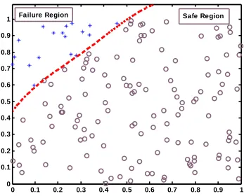
Figure 4-3 SVM reliability analysis training with data size N=10 ... 83
Figure 4-4 SVM reliability analysis training with data size N=50 ... 83
Figure 4-5 SVM reliability analysis training with data size N=100 ... 84
Figure 4-6 SVM reliability analysis training with data size N=150 ... 84
Figure 4-7 SVM reliability analysis training with data size N=200 ... 85
Figure 4-8 SVM reliability analysis training with data size N=250 ... 85
Figure 4-9 SVM reliability analysis training with data size N=350 ... 86
Figure 4-10 SVM reliability analysis training with data size N=400 ... 86
Figure 4-11 SVM reliability analysis training with data size N=500 ... 87
Figure 4-12 Probability of failure vs. Training data size N... 87
Figure 4-13 Training data for linear for case with linear limit state function ... 88
Figure 4-14 Kernel function of Thin Plate Spline for linear Case... 88
Figure 4-15 Spline Kernel function for Linear Case ... 89
Figure 4-16 Cubic Kernel function for Linear Case... 89
Figure 4-17 Quadratic Kernel function for Linear Case ... 90
Figure 4-18 Distance Kernel function for Linear Case ... 90
Figure 4-19 Training data for linear for case with linear limit state function ... 91
Figure 4-20 Radio Basis kernel function for nonlinear Case... 91
LIST OF TABLES
Table 2-1 Point estimation results for natural frequency and damping ratio... 24
Table 3-1 Simulation results for uncorrelated normal inputs - linear case... 49
Table 3-2 Simulation results for uncorrelated nonnormal inputs - linear case ... 49
Table 3-3 Simulation results for correlated normal inputs - linear case ... 50
Table 3-4 Simulation results for uncorrelated normal inputs - nonlinear case ... 51
Table 3-5 Simulation results for uncorrelated normal inputs – nonlinear case... 51
Table 3-6 Simulation results for correlated RVs with different sample numbers ... 52
Table 3-7 The statistics for variates V obtained from sampling number 1,000,000 ... 52
Table 3-8 The statistics for variates V obtained from sampling number 1,500,000 ... 53
Table 3-9 The statistics for variates V obtained from sampling number 1,000,000 ... 53
Table 3-10 Updated probabilistic information of inputs... 59
Table 3-11 Hypothesis test for linear limit state function case ... 60
Table 3-12 Hypothesis test for nonlinear case... 60
Table 4-1 A list of Kernel functions... 76
Table 4-2 Data size vs. Error rate... 79
Table 4-3 Failure probability obtained using different reliability analysis methods ... 79
Table 4-4 Failure probability obtained with different Kernel function – Linear Case.. 80
CHAPTER 1
1 Introduction
1.1 Structural Health Management
Nearly all in-service structures require some form of monitoring to maintain their integrity
and health condition and to prolong their lifespan or to prevent catastrophic failure. The
interest in the ability to monitor the physical condition of a structure and detect damage at the
earliest possible stage is pervasive throughout the civil, mechanical and aerospace
engineering communities. This is now commonly referred to as ‘Structural Health
Management and Damage Detection’.
Structural health management can be defined as the diagnostic and prognostics of the
integrity or condition of a structure. The intent is to detect and locate damage or degradation
in structural components and to provide this information quickly and in a form easily
understood by the operators or occupants of the structure. The damage may result from
fatigue, large earthquake, strong winds, explosion, vehicle impact or other external or
internal loadings or changess. Early detection of damage or structural degradation prior to
local failure can prevent "runaway" catastrophic failure of the system. In engineering
applications, damage is understood intuitively as an imperfection or impairment of the
function and working condition of a structure or machine. Damage can be described in many
ways depending on the structure and its function. Hence damage detection has many
definitions based on what type of damage is being measured [Staszewski, 1998 and Sone,
1995]. Since the health monitoring was defined as use of in-situ, nondestructive sensing and
changes, the term structural health monitoring and damage identification are usually
interchangeable.
Research over the past several decades within the structural engineering and other related
engineering fields have resulted in advancements and technologies that assist structural
engineers in their attempts to ensure the safety and reliability of structures over their life
spans. Two major reasons responsible for this growth of the health management of structural
systems have been: a) the advances in sensors, data acquisition, data communications, and
real-time data analysis, allowing for the implementation of highly reliable and accurate
monitoring and diagnostics hardware with very advanced features [Housner et al., 1997], and
(b) the growing interest in certain markets, such as military, aerospace, and civil
infrastructures, which see the application of health monitoring systems as means of assuring
the correct and safe performance of these engineered systems, as well as protecting their
investments [Chang, 1999]. The structural health monitoring can be performed on both
global and local basis. Global based health monitoring focuses on monitoring and verifying
the performance of the entire system. By monitoring the output, such as vibration
displacement, velocity or acceleration, of the system during its operation, the occurrence of
the damage can be detected. On the other hand, local based health monitoring is interested in
monitoring certain key elements of the total system. The applications of local based health
monitoring usually rely on the use of localized non-destructive evaluation techniques, such as
acoustic or ultrasonic methods, magnetic fields methods, radiography, eddy current methods,
or thermal methods [Doherty, 1993]. All of these experimental techniques require that the
global damage detection methods has led to the development of the methods that examine
changes in the vibration characteristics of the structure.
Damage detection, as determined by changes in the dynamic properties or responses of
structures, is a subject that has received considerable attention in the literature. The basic
idea is that modal parameters (frequencies, mode shapes, etc.) as functions of the physical
properties will cause changes in the modal properties [Doebling et al. 1996]. Damage effects
on a structure can be classified [Doebling et al. 1998] into linear or non-linear. A linear
damage scenario is one in which the linearly elastic behavior of the structure is preserved
after the occurrence of the damage. The changes of modal properties are resulted from the
changes in geometry or material properties of the structure, but the behavior of the structure
can still be modeled using linear equations of motions. On the other hand non-linear effects
are the ones in which the system does no longer exhibit a linearly elastic behavior after the
damage has been introduced. Loosening of fastening elements, where the separation of
mating parts induce non-linear responses in the system, can be cited as these non-linear
effects. Another example of nonlinear damage is the formation of a fatigue crack that
subsequently opens and closes under the normal operating vibration environment.
As mentioned previously, the field of structural health management is very broad. Among
different issues, an important one is to use signal processing techniques, which includes such
methods as Fourier analysis, time-frequency analysis and wavelet analysis. There exist two
major and complementary components that form the basis for structural health management:
hardware or the experimental tools, and methodologies or analytical/computational tools.
Previous analytical and computational studies on damage detection have been tailored toward
modal damping ratios obtained from the vibration signals [Doebling, et al 1996, 1998].
Some of these methods allow for assessing changes in these parameters, which then are
related to some structural damage, but they do not provide information of the exact time of
the occurrence of the damage neither detecting the location of a fault, which may be an
important part in the total picture of what structural health monitoring implies. Methods such
as the windowed Fourier Transforms and Wigner Distribution were among the first
time-frequency methods to be implemented. In recent years, the application of the Wavelet
Transform also provided a new tool for time frequency analysis, which has been effectively
used in health management and damage detection of various structures. In this research
work, different issues involved in the structural health management were investigated. Some
novel ideas to adaptively update system parameters and to obtain system reliability were
explored. In the following sections, backgrounds of different techniques involved will be
introduced.
1.2 System Identification and its role in SHM
System identification is an approach for obtaining an empirical model of a dynamic system
from measured inputs and outputs. Through this process one can find an optimal model
which fits the measured data as well as possible. The model structure is built based on the
prior knowledge and the personal experience of the physical system. According to the prior
knowledge of the physical system, the model structure can be categorized into ‘white box
model’, ‘gray box model’ and ‘black box model’. Among them, the ‘white box model’ has
known properties from the prior knowledge and the physical principles and it not determined
between of the ‘white’ and ‘black’ box model with which, the model structure is built based
on the available prior knowledge with part of the parameters determined from the measured
data. According to the model estimation method, system identification can be classified as
parametric or nonparametric identification. Parametric identification methods are techniques
to find the ‘best’ values of the parameters to make the simulated response close to those from
the measurements. Some commonly used models include ARMAX, ARX and FIR model.
Nonparametric identification methods estimate model parameters without assuming a
parametric model set. Typical nonparametric identification methods include frequency
analysis, correlation analysis and spectral analysis.
In general, changes in the real structures result in changes in the parameters of the structure
models such as stiffness, natural frequency etc. Therefore, adaptively monitoring the
changes of parameters can provide information on structure health condition. The great
potential to apply system identification technique to structural health monitoring and damage
detection has been shown extensively in the literatures. The research work by Saadat et al
[2003] exclusively investigated the application of artificial neural network based system
identification on the damage detection and structural health monitoring. The paper presented
by Beck’s group [2004] introduced a two-stage structural health monitoring approach in
which the first stage was to identify the modal parameters for both the undamaged and
damaged systems. In the second stage of their work, Bayesian system identification was
used to update the structural model. The updated information was applied to decide if the
system was damaged or not. Other noteworthy work can be found in Sohn and Law [2000],
Liu and Rao [2000] to cite a few. To apply system identification technique to structural
and the real system model. Since the occurrence of damage will change the system response
characteristics, the sudden changes in the system are desired to be detected as ‘spikes’. Some
signal processing techniques such as time-frequency analysis and wavelet analysis have been
widely applied to this field to detect structural damage. Literature contributions have been
made by Hou and Noori [1999], Sone et al. [1999], Hou et al. [2000], Noori et al. [2001],
Masuda et al. [2002].
1.3 Structural Reliability Analysis and its role in SHM
The fundamental goal of structural reliability analysis is to determine the safety condition of
the structure. As one of the pioneers to develop the structural reliability, Freudenthal [1947]
introduced the probabilistic theory to deal with structural safety issue. The researchers have
studied this area over half centaury. Nowadays, the probability of failure has been one of the
most important notations of the structural reliability. The traditional methodology of
structural reliability is achieved by deterministically finding the design point according to
some conservative assumptions. The theory of first reliability method (FORM) and second
reliability method (SORM) was significantly improved by 1990 (Rackwitz, 2001). These
two methods work by linearizing the limit state function at the design point which is the most
possible failure point in the failure region. The simplicity and efficiency of these methods
make them widely recognized in both academic and industrial fields. However, to use these
methods, structural model is usually oversimplified to build up a limit state function. And
more importantly, it is not applicable for some cases like non-asymptotic case. On the
contrary, the Monte Carlo Simulation (MCS) method, another widely used structural
probability of failure. In 1983, Importance Sampling was introduced by Harbitz (1983) to
perform reliability analysis. Importance sampling is a method that has some of the features
of both FORM/SORM method and numerical Monte Carlo Simulation method, in which,
sampling is performed close to the design point. It is more accurate and efficient for certain
cases compared to FORM/SORM. The reliability analysis methods discussed herein have
their own advantages. The detail application of these approaches will be introduced in the
third chapter.
In practical world, structural safety and reliability is crucial for assuring sustainability of
infrastructure systems and thus, economic benefits and saving lives. For certain structures, it
is often required to calculate and predict the structural reliability and safety during their
service life. In Wong & Yao (2001), the “value chain” concept was introduced in a holistic
view of structural health management, with which the data interpretation, damage detection
and structural reliability estimates were viewed as sequential components in a value chain.
Among them, structural reliability and useful life expectancy are seen to be the crucial parts
to realize the full value of the chain.
The ultimate goal of structural health management is to achieve a significant improvement in
structural reliability. Even though techniques of structural health management have been
extensively developed during the last decades majority of the literatures in this area is
focused on how to collect information and detect the damage. More attention needs to be
paid to integrate the current state of the structure health with reliability schemes to improve
the service life of a structure. The ultimate goal of this research is to develop an adaptive
technique that can be utilized to obtain the up to date system information. This technique can
1.4 Bayesian Based Probabilistic Analysis
Bayesian theorem is a probabilistic theorem derived from the basic sum and product rules of
probability theory. Traditionally, probability is interprated by the frequeny that an event
happed in a large number of similar trial samples. The events happed are considered as the
different realization of a random variables. In contrast to the frequency based probability
theory, Bayes’ theorem brought up another way to interpret probability. Firstly presented by
Thomas Bayes in 1763, Bayes’ theory interprets probability in terms of a certain degree of
belief. A Bayesian probabilistic approach is a powerful way to formulate a model to describe
the system of interest. It provides a rational basis to combine subjective priori information
and objective system measurements. The posterior probability density function (pdf) of
interest can be obtained by adapting the predefined priori pdf based on the observed
information.
Classic inferential model do not permit the introduction of the prior knowledge into the
calculation. However, some of the prior knowledge includes numerous useful information.
It is often a desire to address a question with regarding to the past pertinent knowledge and
newly collected data. Bayesian analysis provides such a logical, quantitative framework to
combine prior and new data for inference. Inference means computing the probability
distribution for a set of unknown variables from a set of known variables. The observing of
this set of known variables form a distribution called the likelihood function. The
characteristics of the variables are considered to have its own probability distribution which
is the previously described priori distribution. Because of its process to update the
analysis is often referred to as an updating algorithm, with which new information is
obtained using the existing information and some subjective assumption.
With the history of more than two century, a lot of attentions were addressed to Bayesian
approach during 1950s and 1960s by researchers. Over the past decade both in the statistical
fields and the methodology developments different areas of application of Bayesian theory
have been actively explored. A variety of modern technologies are influenced broadly by
Bayesian thinking which include the field of computer science, bioinformatics, economics,
medicine, physics and so on (Fienberg, 2006; Poirier, 1988). The application of Bayesian
approach to data analysis is of particular interest in this research work. It was first applied to
system identification and structural damage detection. By utilizing the property of its
functionality to model system parameters as random variables and its ability to incorporate
subjective knowledge into system measurements, Bayesian analysis was used to model the
system uncertainties and update the system information. The details of these works will be
presented in the following chapters.
1.5 Support Vector Machine Learning Algorithm
In practice, structural systems under investigation always have certain complexity. Their
behavior is either difficult or unlikely to be predicted under harsh environment. Similar to
artificial neural network which has been used to model structural behavior, Support Vector
Machine (SVM) possesses the well-known ability of being a universal approximator for any
multivariate function to any desired degree of accuracy (Kecman, 2005). The SVM has
become a promising algorithm and has gained popularity during the last decade.
Technically speaking, Support Vector Machine (SVM) is a statistical learning algorithm for
developed by Vapnik, Chervonenkis and their co-worker’s back in 1960s (Vapnik and
Chervonenkis, 1968). Unlike the traditional statistical inference, SVMs are so called
‘nonparametric’ models, which means the parameters involved in SVM are not predefined
and their numbers depend on the training data used. A hyperplane is one that separates
between different sets of objects having different class characteristics. A special property of
Support Vector Machine classifier is to simultaneously minimize the empirical classification
error and maximize the geometric margin. Therefore SVM is also known as maximum
margin classifier.
During the past years, SVMs has been applied to various domains including handwriting
recognition, speaker identification and text categorization and so on. In practice, structural
systems being investigated always have certain complexity. Their behavior is either hard to
predict using mathematical models or changing due to upgrade or redesign. A SVM based
reliability analysis technique is introduced in this research work to classify safe condition and
failure condition by utilizing a pre-trained hypothesis function. As it will be shown in the
following chapters, the proposed SVM based reliability developed in this research is proved
to be a time saving method compared with Monte Carlo Simulation and leads to more
accurate results compared with other traditional reliability analysis techniques such as first
order reliability method and second order reliability method. More over, in reality, due to the
lack of complete knowledge about the structure or the changes in the characteristics of the
structure through time, such as upgrades and redesigns, the information to define a
reasonable limit state function could be limited and sometimes non-continuous. It is another
CHAPTER 2
2 Bayesian Based System Identification
2.1 System Identification
System identification is about to build and evaluate a mathematical model of a system
according to its input and output measurements. A system usually refers to a dynamic
process to produce observable signals by the interaction of the different variables. With the
development of the control theory, system identification was well developed and
significantly applied to the control field. Over the past two decades, the different techniques
of system identification have been well established and broadly applied to many different
fields. Those different fields include financial analysis, speech system analysis and so on.
The related literatures can be found in Lois (1997) and Nickel (2005).
Usually, there are different shapes of models available for a dynamic system according to
different complexities. The key problem of system identification is to find the most suitable
model for the physical system among the cluster of models. This model is considered as the
optimal one with which it is simple enough to evaluate and accurate enough to capture the
desired model behavior. A model reflects the relationship between system input and output.
The system output is partially determined by the input because of the effects of
environmental disturbance or other uncertainties. A general concept of a dynamic system
model can be shown from Figure 2-1. A model is mathematically constructed according to
the priori knowledge of the system dynamics and the assumptions according to the physical
insights. “White Box”, “Gray Box” and “Black Box” are three color coded levels to describe
• “White Box Model” is built by the already known properties from the prior
knowledge and physical principles. It is determined ideally from full knowledge of
all components of the physical system instead of the measured data. The application
of white box model is limited sometimes because of its complexity or limitation to
obtain the fully required prior knowledge.
• “Gray Box Model” is built based on the available prior knowledge with part of the
parameters determined from the system measurements. With this kind of model, a
relatively simple structure can be obtained from the prior knowledge and system
observation can be used to estimate the remaining unknown system parameters. • “Black Box Model” is opposite to the ‘white box model’ and is fully determined by
the measured data with little prior knowledge. The characteristic of analyzing the
dynamic system without knowing the physical insight draws a lot research interests
to black box system identification. There are varieties of literatures to cover topics
from mathematical estimation theory to different algorithms including neural
networks, fuzzy models and wavelets system identification and so on. The related
literatures are Gupta and Sinha (1998), Haykin (1999), Nelles (2001), Judisky and
Hjalmarsson et. al (1995) and Ashino, Mandai and Mrimoto (2004).
From the above introduction, it is easy to see that finding a model for a dynamic system
according to the three color coded approaches is case dependent. Models built from different
priori information usually come with varieties of formats. Different techniques to evaluate
the model can be categorized into parametric and nonparametric system identification
It is the intention of system identification to find the “most” suitable model structure for the
dynamic system and to find the “best” value for the model structure. Parametric system
identification method refers to techniques that estimate the parameter values for a given
model. The application basis of parametric system identification is the determination of the
system model. Once the model is defined, the process of finding the optimal value for system parameter vectors θ becomes the problem of parameter estimation. With the
measured system input and output data, the optimal values for the system parameters are
determined by the certain criteria, usually known as the prediction error:
( ) ( ) ( )
θ θε t, = y t −yˆ t| (2.1)
The process of finding the “best” model is the process to minimize the prediction error. A
quadratic norm is typically chosen as a standard candidate of the error cost function due to its
convenience for computation and analysis:
( )
∑
( )
=
= N
t
t N
l
1 2
, 2
1 ε θ
ε (2.2)
There are varieties of ways to fit the model to the measured input-output data by minimizing
the error cost function. Among them, Linear Regressions and the Least-square Method and
the Maximum Likelihood Method are the most frequently used techniques (Ljung, 1999).
The Least-square method has its unique feature to analytically find the optimal values. The
Maximum Likelihood method is the one with statistical feature and will be studied and
implemented in this research work.
Let random variables represent the N measured data from the system, θ
denotes the M unknown parameters of the system. The likelihood function of the system
generally refers to the probability distribution function of unknown model parameters given N
N
y y y
the system measurements. Herein, the probability density function is used to make the
expressions more explicit:
(
N |θ)
(
1, 2, , N |θ)
y y f y y y
f = L (2.3)
An estimator is often used to accomplish the parameter estimation task by utilizing the
observable . The estimation is performed by finding values which maximize the
logarithm of the estimator:
(
Ny
θˆ
)
)
Ny
( )
(
θθ
θ |
max log
ˆ N
y N
ML y = f y (2.4)
Maximum likelihood method is a powerful method but it requires large sample size to obtain
precise estimation. This method can be improved by integrating that with Bayesian approach
as presented in section 3 of this chapter.
Nonparametric system identification techniques try to find an optimal system model without
knowing the system parameters explicitly. Typical time domain methods include Impulse
Response method, Step-Response analysis and Correlation analysis. The frequency domain
methods include sine-wave testing method, Correlation analysis, Fourier analysis and
Spectral analysis (Ljung, 1999). Those methods can be implemented both to the linear or
non-linear systems depending on the different cases.
In practical world, system identification can be considered as an experimental process to
estimate model parameters until its output matches with the observed physical system output
as well as possible. The procedures of system identification include following basic steps:
o Selection and definition of model structure: As a mathematical representation of a
structure, a suitable model is chosen using priori knowledge, application of identification
and trial processes.
o Choice of a criteria of fit: Finding an optimal model of the system according to a given
criteria, which reflects the quality of the model about how well it fits the measured data.
o Parameter estimation: Finding numerical values of the model parameters. This is an
optimization problem.
o Model validation: Even though the model selected is considered as the best one to represent the system, the model still needs to be tested to reveal any deficiency.
Even if the model parameters obtained through this procedure are their optimal values, it may
still not be possible to duplicate the behavior of the structures exactly. This is because of the
so-called modeling error. Besides, the measured data is usually with a finite number and
associated with environmental disturbance and measurement noise. This may induce the
variation of the estimated value from this true value. This part of the variation is knows as
the variance error. Both modeling error and variance error introduce the uncertainties to the
system identification process. In many applications such as aircraft and machinery health
management, the consideration of these uncertainties is especially important.
Over the past century, techniques for system identification have been developed and
implemented to various application fields. Major focuses of the techniques include the
development of methodologies/algorithms which can adapt the model structures to different
dynamic systems, and the data acquisition techniques for capturing the high quality
input-output data/information. During last decades, an evolving area for improving both of these
“intelligent” way. The subsequent actions that need to take place in order to acquire the
integrity of the system subject to the external environment and/or loading conditions. A
critical and essential requirement for in-depth understanding of the nature of changes
encountered in the system is the identification of the system’s model, and thereby the update
of the knowledge about the changes in its dynamic characteristics. In order to address these
important factors, the application of probabilistic techniques to identify and update the
knowledge about a structural model has emerged as an active research area in recent years
(Sohn and Law, 1997; Beck and Au, 2002). Due to its importance in data analysis, the
Bayesian probabilistic system identification approach has received growing attention in
recent years. Specific techniques such as the Markov chain Monte-Carlo method in Bayesian
system identification have been explored by different researchers (Ninness and Brinsmead,
2001; Kerschen, Bolinval etc., 2003). Model updating for both linear and nonlinear systems
have been investigated by Beck and Katafygiotis (1998), Yuen and Beck (2001). In this
research work, the effects of different prior pdfs and amounts of available data were
investigated. Following a brief introduction to the Bayesian system identification approach,
numerical simulations will be presented in order to demonstrate these effects.
2.2 Fundamentals of Bayesian Analysis
Bayesian inference is statistical inference in which uncertainties are interpreted in terms of
probabilities with degrees of belief. A Bayesian probabilistic approach is a powerful way to
formulate a model to describe the system of interest. After observing some data, the
“posterior” probably density function (pdf) can be obtained by adapting the predefined
Traditionally, probability is interpreted by the frequency that a certain event happed in a
large number of trial samples. Bayes’ theorem was first presented by Thomas Bayes in 1763.
In contrast to the frequency based probability theory, Bayes’ theorem brought up another
way to interpret probability.
In a statistical view, let H stands for a hypothesis that contains the information before the
observation. E stands for the new observation or event. According to the probability product
rule, the joint probability is defined from the conditional probability:
(
E,H)
P(E|H) P(H) P(H |E) P(E)P = × = × (2.5)
As a well-known theorem, Bayes’ formula is actually a derivation of the above product rule
and its expression is as follows:
) ( ) ( ) | ( ) | ( E P H P H E P E H
P = × (2.6)
In formula (2.6), P(H) is usually called the prior probability of H, P(E|H) is the likelihood
function and P(H|E) is the posterior probability of H given E. The corresponding marginal
probability can be obtained from the following equation:
dH H E P E
P
∫
+∞∞ −
= ( , ) )
( (2.7)
The marginal probability is usually considered as a normalizing factor. To reduce the
computation effort, for the cases that only the hypothesis part is of interest, the marginal of
P(E) can be omitted and Bayesian theorem can be expressed in its proportional form:
) ( ) | ( ) |
(H E P E H P H
P ∝ × (2.8)
For the cases with more than two random variables, Bayes’ theorem can be rewritten as:
) ( ) | ( ) , | ( ) , |
(H E1 E2 P E1 H E2 P E2 H P H
With as many as of N random variables, the chain rule of proability is applied, and the
Bayes’ formula is written as the following form:
) ( ) | ( , , ) , , , | ( ) , , , |
(H E1 E2 E P E1 E 1 E1 H P E2 H P H
P L N ∝ N− L ×L× × (2.10)
In general, probability density function is the basic way to define a continuous random
variable. Therefore, it is more convenient to perform Bayesian analysis using probability
density function. A derivation from the probability distribution to probability density can be
found in Papoulis (1984). The Bayesian theorem for probability density function is
illustrated as in the following equation:
) ( ) ( ) | ( ) | ( | | E f H f H E f E H f E H H E E H × = (2.11)
The proportional form for the probability density function is as follows:
) ( ) | ( ) | ( |
| H E f E H f H
fHE ∝ EH × H (2.12)
The generalized N random variables expression is:
) ( ) | ( , , ) , , , | ( ) , , , |
( 1 2 | 1 1 1 | 2
| H E E E f E E E H f E H f H
fHE L N ∝ EH N− L ×L× EH × H (2.13)
It was shown from above introduction that the general strategy of Bayesian analysis is to
utilize the decomposition property of the conditional probability. The application of this
theory is based on the assumption that the uncertainties modeled can be interpreted by certain
probabilistic form. In the following section, a method of Bayesian based system
identification is introduced. The statistics of system parameters are considered as the random
variables with assumed pdfs. The posterior pdfs of those parameters are updated according
2.3 Bayesian Analysis Based System Identification
In Bayesian statistics, probability is interpreted as a rational measure of belief that is used to
describe mathematically the uncertain relation between the statistician and the external world
[Peterka, 1981]. Bayesian approach based system identification is thus different from the
classical system identification conceptually. In Bayesian approach, the parameters to be
evaluated are considered as random variables. The desired parameters can be inferred from
the system measurements of other random variables and the likelihood function, which builds
up the connection between the unknown and the observable parameters.
Suppose that θ is a finite set of parameter to be studied, YN is the measurement from the
system, the equation (2.12) can be rewritten as:
) ( ) | ( ) | ( | | θ θ θ θ θ
θ Y f Y f
f Y ∝ Y × (2.14)
Where, )fθ(θ is the predefined prior probability density function that represents the previous
knowledge of the system, and fY|θ(Y |θ)
) | ( Y f
is the ‘likelihood function’, which reflects the
‘likelihood’ that the observed event should indeed take place [Ljung, 1999]. The prior
information is modified according to the up to date measurements to obtain the current sate
knowledge of the system, which is the posterior probability density function θ|Y θ . The
generalization multi-variable form for equation (2.14) is as follows:
) ( ) | ( , , ) , , , | ( ) , , , ,
( 1 2 | 1 1 | 1
, θ θ θ θ θ θ θ
θ Y Y Y f Y Y Y f Y f
f
N N
N N Y N N Y
Y L ∝ − L ×L× × (2.15)
Bayesian approach is applied to system identification because of its simplicity and stochastic
feature. By utilizing this probabilistic theory, a degree of belief can be assessed for a system
basis of subjective assumption and with the condition of the current available observations.
The Figure 2-2 is a summarization for the principle of the Bayesian system identification.
As discussed already, the priori pdf is generally assigned subjectively according to the
exiting knowledge of the system parameters. There could be varieties of choices since it is
based on the selected choice. The effects of different assignments will be checked in the
following section by performing numerical simulations. It is shown that the critical part for
Bayesian based system identification is the definition of the likelihood function. A proper
form of the likelihood function is the one that not only builds up the connection between the
parameters of interest and the system observables, but also provide an explicit mathematical
formulation to reduce the computation cost. This term usually depends on the dynamic
system and is also probabilistic based. In this Bayesian based approach, the external
disturbance is incorporated into the system measurements. By performing basic conditional
rules, it can be distinguished from the system model and evaluated separately if needed.
Since the parameters of interest to be evaluated are obtained in probability distribution forms,
the problems like prediction error could be irrelevant. The advantage of Bayesian approach
to consider the unknown parameters as random variables is the feature that provides a
rational basis for problem decision making (Peterka, 1981). Decision making is to choose an
optimal point with which the system model can be best described. From the statistical view,
the probability density associated with any variable is a measure of confidence that lies in the
neighborhood of the mean value. The optimal estimation of the parameter is given by
maximizing the posterior pdf as in equation (2.16).
)) | ( max( ˆ
|Y YN f
N θ
In traditional system identification, the estimated parameter is one single value with the
problem being processed in one shot. With Bayesian system identification, the adaptability
of the method makes it possible to obtain the up to date system parameter information based
on the current state observation. In general, changes in the real structures are reflected by
the system output measurements, which induce the changes in the parameters of the structure
models such as stiffness, natural frequency, etc. Therefore, adaptively monitoring the
changes of system parameters can monitor the system change and provide information on the
structural health conditions. This will be the potential application of the Bayesian based
system identification to structural health management. In the following section, different
issues including effects of priori selection, data sizes and sample conditions on Bayesian
system identification will be addressed through the numerical simulation cases.
2.4 Numerical Simulation
As stated previously, system identification is to find a mathematical model for a physical
system. This model should be good enough to describe the certain behavior of interest and
simple enough to reduce the computation cost. In this research work, the ultimate goal is to
study the system health condition and to improve the structural reliability, thus system
models with specified parameters are the major concern. Therefore, it is a task of
statisticians to solve a parametric system identification problem and to extract information
according to their past experience and current observations. To start with a general example,
the Bayesian system identification approach is applied first to a single degree of freedom
mass-spring-damping system and further extended to a three-story-shear building.
A dynamic structural system is usually described by the equation of motion. The natural
change of the system natural frequency implies the change of the whole system. Hence it
will be the main task to deal with those parameters in the following sections. To be
consistent, let θ=<ζ,ω>. For a physical system, with a statistically simulated sample input,
the output can usually be observed as YN. The choice of the priori pdf will be discussed in
the following numerical cases. The choice of the likelihood function is critical though and it
is often desired to build up the relationship between the system parameters and the system
observables. This function is generally system dependent. For the systems to be studied
herein, they are both linear systems with stationary Gaussian excitation. In such situation, a
Gaussian distribution is commonly assigned to the probability density of YN given the system
parameters. Gaussian is one of the most import distributions in probabilistic family. Many
physical measurements can be well approximated by it even though the underlying
mechanisms are different. The general form of its probability density function is:
⎥⎦ ⎤ ⎢⎣ ⎡− − = 2 2 2 ) ( 2 1 exp 2 1 ) , | ( µ σ π σ σ µ x x f (2.17)
The N-variant Gaussian density function with mean X and covariance matrix Σ is expressed
as: ⎥⎦ ⎤ ⎢⎣ ⎡− − Σ − Σ = − ) ( ) ( 2 1 exp ) 2 ( 1 ) , ,
( 12 1
2
1 X X X X X
X f T N N X π L (2.18)
For the current case, X is replaced by the output of systems YN. Since the likelihood function
is desired to be a probability density function of YN given system parametersθ, the chain rule
as in equation 2.15 needs to be applied to obtain the following equation:
( )
θ(
θ)
θ θ θ
θ ( | ) | 1, 1,
1 | | − =
∏
×∝ k k
N
k Y N
Y Y f f Y Y Y
At this stage, the problem turns out to be a recursive parameter estimation problem. The
least square function was used as the error cost function. A point estimator as discuss in
equation 2.4 was used to find an optimal value of the parameters when needed. In the
following part, the numerical results will be demonstrated and discussed.
2.4.1 Case study for a single degree of freedom system
The first simulation was done based on a SDOF oscillator characterized by the equation of
motion: x&&+2ζωnx&+ωnx=−f(t), where ζ is the damping ration and ω
2
n is the natural
frequency. The configuration of the system is shown in Figure 2-3. The system is subject to
the white noise excitation f(t). The exact parameters used to generate simulation data YN
areθv =[ωn,ζ]=[3,0.02]. To calculate the desired posterior pdf of the system parameters
) | ( Y
fθ|YN θ N , the autocorrelation θ
[
τ θ]
v| ) ( ) ( )
,
(Y EY t Y t
RYY = + of the system response have
to be evaluated. This part is the key factor to determine the likelihood function, thus it is of
particular interest to analyze this first. From the definition of autocorrelation, it gives the
information of dependency from one measurement Y(t) to the next time series of the system
Y(t+τ).
In Figure 2-4, the system excitation, the resulted system output and its correlation plots are
plotted respectively. In the first step of the simulation, Gaussian pdf was assumed for both
natural frequency and damping ratio. Posterior profile for single parameter was obtained
given the other parameter was known. In Figure 2-5, the resulting posterior probability
density function for natural frequency fθ|Y (ωn |YN,ζ =0.02)
N and damping ratio
) 3 ,
| (
|Y YN n =
f
N ζ ω
The optimal values obtained using maximum likelihood estimator were compared with the
corresponding exact values. The standard deviations obtained from the statistical form are
listed in Table 2-1. Error rates are also listed out in the table.
Table 2-1 Point estimation results for natural frequency and damping ratio
Parameters Exact Value Optimal Estimation Error Rate Standard Deviation
Natural Frequency ωn 3 rad/s 3.12 rad/s 0.04 0.0036
Damping Ratio ζ 0.02 0.02005 0.0025 0.0004
From the data illustrated in the above table, it is shown that the system parameters estimated
using Bayesian based system identification method are all in 5% of error range and accurate
enough to be accepted.
Different Prior: To check results dependence on the priori distribution, simulations based on
three different priori pdfs were performed to obtain the posterior pdfs. The results are plotted
in Figure 2-6, Figure 2-7 and Figure 2-8.
In Figure 2-6, a uniform priori was defined for the natural frequency and the corresponding
posterior pdf was obtained by performing the analysis. It is shown that the priori and
posterior are in different form. Same phenomena happened to Rayleigh and even normal
priori definition. In Figure 2-9, pdfs obtained using the previous 3 priori pdfs are plotted in
one figure and obviously there are in close shape even though coming from totally different
priori definition. At this stage, it is safe to state that the prior information defined
subjectively has been corrected by the objective system observables. In the rest of this
research work, the uniform priori was used because of its simplicity.
data acquisition is usually limited by physical memory, time to consume, data transmission
and so on. Therefore it is always desired to find an optimal number of data lengths to
balance the trade off between data information carried by data length and the accuracy of the
system model. In Figure 2-10, results obtained from different data length N=10, N=25,
N=100, N=1000 are illustrated. It is obvious that N=100 is a sufficient number to validate
the result.
Different Data Sets: Similarly to the case stated in the above discussion, it is desired to have
more objective information from the physical system to interpret the system characteristic
more accurately. In practical situation, it is possible to have different sets of independent
measurements. Hence it is worthwhile to check the effect of statistical sampling with 1 data
set and more data sets. In Figure 2-11, 4 sets of independent samples were used to compare
with the results using only one set of data. In the figure, the green line was obtained by
taking the average of the pdf from 4 sets of data. It is shown that the optimal value using more data becomes closer to the actual value of ωn. The width of the posterior pdf also
becomes narrower with larger data. It indicates that the confidence has been increased in the
estimation.
Cumulative Distribution Function: Probability distribution function is calculated from
probability density function. It is more straightforward and contains information of mean
and variance which might not be reflected in pdfs other than Gaussian distribution. It can act
as a tool to evaluate the consistency of predicted pdf and the sample data. In the current case,
results are plotted in Figure 2-12 and it shows the cumulative distribution function (CDF)
Joint Probability Function: For systems with more than one parameter to be identified, the
posterior pdf evaluated can be in the form of joint probability density function. To obtain the
optimal values of the parameters, one way is to perform integration to obtain the marginal
pdf and evaluate the parameter according to this resulting pdf. The other way is to extract the
parameter information directly from the joint pdf. Figure 2-13 – Figure 2-18 illustrate the
surface plots of the joint probability and the corresponding contour plots. These plots were
based on data generated with different time step. It is shown that with finer time step, the
information extracted can be more close to the actual value.
2.4.2 Three-story-shear building
To further explore the feasibility of this proposed approach on a higher degree of freedom
system, a three-story-shear building, shown in the Figure 2-19, is employed. The equation of
motion for this structure is:
( )
t F Ky y C yM&&+ &+ =− (2.20)
Where M, C and K are mass, damping and stiffness matrix respectively. F(t) is the base
excitation with Gaussian distribution. The original configuration of the structure is: m1 = m2
= m3 = 10kg, k1 = 28 kN/m, k2 = k3 = 24 kN/m and the damping ratio is chosen to be 2%. By
performing the general modal analysis techniques, the uncoupled modal equations can be
obtained. Therefore, the Bayesian system identification procedure can be applied for the
MDOF system in the same way as application to the SDOF system.
In Figure 2-20, the conditional posterior pdf is obtained by using the
displacement measurement from the 1
) | (K1 YN prob
st
floor. The actual value of the stiffness in the first
0.007. The corresponding standard deviation is evaluated as: σK = 0.0055. The error rate
falls to 5% range, hence it can be considered as an acceptable estimate.
In some cases, more than one parameters need to be identified. For example, stiffness of
both the first and second floor is to be evaluated. The resulting posterior pdf is
two-dimensional since it is a function of both K1and K2. Figure 2-21 is the contour plot of it with
the contours corresponds to 10 percentage levels of the maximum probability.
2.5 Conclusions:
In this part of the research, a Bayesian system identification approach was introduced and
demonstrated. The unknown parameters of dynamic systems were accurately estimated by
optimizing the conditional posterior pdf. The associated covariance of the pdf was used to
quantify the uncertainty. The choice of prior pdf has minor effects on the posterior pdf. By
increasing data availability, the confidence of estimations can be increased. From the joint
probability density function of different parameters, parameter information could be
extracted from the contour plot. However, it was restricted by the data size. For more than
two parameters, this will encounter the problem of visualization. In future studies, one may
consider defining a different likelihood function with parameters independent of each other
Disturbance e(t)
Dynamic System
Input u(t) Output y(t)
Figure 2-1 A General system model structure
1 2 3 4 5 6 7 8 9 10
Priori pdf: fθ(θ)
Measurement YN
Posteriori pdf:fYN|θ(θ |YN) )
| (
|θ N θ
Y Y
f
N
Likelihood Function
Disturbanc
Bayesian System Identification Process
Figure 2-2 Principle for Bayesian system identification
c
m k
F(t)
0 1 2 3 4 5 6 7 8 9 10 -10 0 10 Time (sec) Ex c it a ti o n
0 1 2 3 4 5 6 7 8 9 10
-0.2 0 0.2 Time (sec) S yst e m O b se rv a ti o n
0 10 20 30 40 50 60 70 80 90 100
-5 0 5
R YY
Figure 2-4 Excitation and Autocorrelation of the system
2.7 2.8 2.9 3 3.1 3.2 3.3 3.4 3.5 3.6 0 0.2 0.4 0.6 0.8 1
Weighting for Natural Frequency ωn (rad/s)
P o s teri o r pdf : prob( ω n |Y N ,ζ )
-0.040 -0.02 0 0.02 0.04 0.06 0.08
0.2 0.4 0.6 0.8 1
Weighting for damping ratio ζ
P o s teri o r pdf : prob( ζ |Y N ,ω n ) Posterior pdf Optimal value Posterior pdf Optimal value