Optical Waveguide Modelling Based On Scalar Finite Difference Scheme

Jurnal Teknologi, 42(D) Jun. 2005: 41–54 © Universiti Teknologi Malaysia

1,2&3

Photonic Research Group, Faculty of Electrical Engineering, Universiti Teknologi Malaysia, 81310 Skudai, Johor.

Email: [email protected], [email protected], [email protected]

OPTICAL WAVEGUIDE MODELLING BASED ON SCALAR FINITE DIFFERENCE SCHEME

NORAZAN MOHD KASSIM1, ABU BAKAR MOHAMMAD2, & MOHD HANIFF IBRAHIM3

Abstract. A numerical method based on scalar finite difference scheme was adopted and programmed on MATLAB® platform for optical waveguide modeling purpose. Comparisons with other established methods in terms of normalized propagation constant were included to verify its applicability. The comparison results obtained were proven to have the same qualitative behaviour. Furthermore, the performances were evaluated in terms of computation complexity, mesh size, and effect of acceleration factor. Computation complexity can be reduced by increasing the mesh size which will then produce more error. The problem can be rectified by introducing the acceleration factor, Successive Over Relaxation (SOR) parameter. It shows that SOR range between 1.3 and 1.7 can give shorter computation time, while producing constant value of simulation results.

Keywords: Optical waveguide, waveguide modelling, finite difference technique, successive over relaxation

Abstrak. Pemodelan pandu gelombang optik telah dilakukan dengan kaedah berangka berasaskan pembezaan skalar terhingga menggunakan peraturcaraan MATLAB®. Perbandingan dengan kaedah-kaedah lain telah dijalankan bagi menilai kebolehupayaannya dalam pemodelan tersebut. Keputusan perbandingan menunjukkan ciri-ciri kualitatif yang sama antara kaedah-kaedah tersebut.Prestasi kaedah ini juga telah dinilai berdasarkan kepada kerumitan pengiraan, saiz jaring dan kesan faktor cepatan. Kerumitan pengiraan boleh dikurangkan dengan menambahkan saiz jaring tetapi ini akan menambahkan ralat pengiraan. Masalah ini boleh diatasi dengan memperkenalkan faktor cepatan iaitu parameter SOR. Ditunjukkan bahawa julat SOR di antara 1.3 dan 1.7 akan menghasilkan masa pengiraan yang lebih singkat dan keputusan simulasi yang lebih konsisten.

Kata kunci: Gelombang optik, pemodelan pandu gelombang, kaedah berangka berasaskan pembezaan skalar

1.0 INTRODUCTION

photonic integrated circuits utilize the channel waveguides as a fundamental component. The waveguides can be in various transverse structures which include the rib, strip, embedded, strip loaded, and buried type. Many critical steps may involve during these waveguides development process. Undoubtedly, the most basic and important step is the modelling process. The modelling process plays significant roles in the advancement of optical waveguides and components by evaluating the structural design performance such as waveguiding and mode confinement capability. In addition, it will reduce the high cost that is required during the fabrication process by optimizing the design that best suited the initial requirements. Furthermore, less time is consumed as no repeated process of fabrication will be needed.

Modelling techniques can be divided into analytical and numerical methods. Numerical methods are preferable in waveguide modelling process due to certain drawbacks of former methods as mentioned in [1]. For the numerical techniques, various approaches which include the scalar and vectorial finite difference [2-4], scalar and vectorial finite element [5] and beam propagation method [6] are applicable. Amongst, finite difference method is preferred due to easier programming task while producing acceptable simulation results, which has been verified previously [2]. However, accumulation of truncation error during implementation may reduce the method’s effectiveness [7]. According to Sadiku [7], this error can be reduced by mesh size reduction but this will definitely increase the computation time, which is not of our interest. In order to rectify this problem, works has been initiated by analyzing the effect of mesh size and acceleration factor. Extensive analysis has been done in order to produce acceptable simulation results while shortening the period.

2.0 THEORY

The basic formulation that governs the propagation of light in the optical waveguide is a Maxwell’s equations that consist of the following [6]:

d B E

dt d D

H J

dt .B

.D ρ_ν



∇ × = − _

 

∇ × = + _



∇ = 



∇ = _

0

(1)

where:

E : electric field intensity

D : electric field density

B : magnetic field density

v

ρ : electric charge density

J : current density

Assuming that the waveguide is made of isotropic, homogeneous and free of source medium, Equation (1) will become:

0 0

d B E

dt d D H

dt .B

.D



∇ × = − _

 

∇ × = _



∇ = 



∇ = _

(2)

Manipulating Equation (2) will produce a so-called Helmholtz wave equation that adequately describes the propagation of electromagnetic wave. The wave equation for the electric field can be presented as:

d E dt

E µε

∇2 = 2

2 (3)

Considering a y-polarized TE mode which propagates in the z-direction and β as a

propagation constant in longitudinal direction will then yield:

y y

y y

d E d E

E E

dx + dy −β = −ϖ µε

2 2

2 2

2 2 (4)

Taking _k2 ₌ϖ2µε _{as the total propagation constant which combine the horizontal}

and vertical part will then produce:

(

)

y y

y

d E d E

k E

dx + dy + −β =

2 2

2 2

2 2 0 (5)

Knowing that k is a multiplication of free space propagation constant, k₀and refractive

index, n for respective layer, Equation (5) can be written in the form of:

(

)

y y

o y

d E d E

k n E

dx + dy + −β =

2 2

2 2 2

2 2 0 (6)

Equation (6) is the eigenfunction that need to be solved for determining the eigenvalue

In the application of finite difference method to solve Equation (6), the E field and

the refractive index, n, is considered to be a discrete value at respective x- and y

-coordinate and bounded in a box, which represent the waveguide cross section. The

box is divided into smaller rectangular area with a dimension of ∆xand∆y in x- and

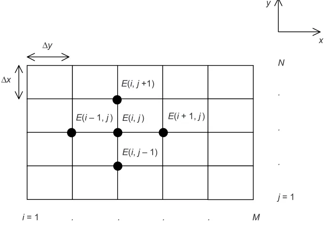
y- directions respectively [8]. Brief description is given in Figure 1, where the waveguide

cross section area is divided into M × N grid lines, which corresponds to the mesh

size of∆xand∆y.

Considering the Eyhaving component in x and y direction E(x,y), Taylor’s expansion

is applied to Equation (6) where the differential components are obtained as follows:

(

)

(

)

( )

(

)

(

)

( )

2

2 2

2

2 2

1 1 2

1 1 2

E i , j E i , j E i , j d E

dx x

E i , j E i , j E i , j d E

dy y

+ + − − 

= _

∆ 



+ + − − _

= _

∆ _

(7)

Combining Equations(6) and (7) will produce a basic equation for obtaining the electric field:

Figure 1 Presentation of the axis, meshes and grid lines for the finite difference calculation y

E(i – 1, j)

∆y

j = 1

i = 1

N

M

x

∆x _{E(i, j +1)}

E(i, j)

E(i, j – 1)

E(i + 1, j)

. . . .

.

.

( )

(

)

(

)

(

(

)

(

)

)

( )

(

)

x

E i , j E i , j E i , j E i , j

y E i , j

x

x k n i , j

y β ∆  + + − +_{ } + + − ∆   =  _{∆ }   +_{ } − ∆ −  _{∆ }    2 2 2 2 2

2 2 2 2

2

1 1 1 1

2 1 (8)

where i and j represent the mesh point corresponding to x and y directions respectively.

If Equation (6) is multiplied with Ey and operating double integration towards x

and y, it will yield:

2 2 2 2 2 2 2 2 y y

y o y

y

d E d E

E k n E dxdy

dx dy E dxdy β    _ + _+  _{ }    =

∫∫

∫∫

Equation (9) is called Rayleigh Quotient. Further application of finite difference method and trapezoidal rule to Equation (9) shall then produce:

( )

(

)

(

)

( )

(

)

(

)

( )

( ) ( )

( )

1 1 2

1 1 2

M N

i j

o

M N

i j

E i , j E i , j E i , j x

E i , j E i , j E i , j

E i , j x y

y

k n i , j E i , j

E i , j x y β − − = = − − = = + + − −  ₊  _∆    + + − +  _{+ ∆ ∆}  _∆        = ∆ ∆

∑ ∑

∑ ∑

Equation (10) is obtained by applying Dirichlet boundary condition which states

the E(i, j) = 0 at the boundary. Initial value of E(i, j) = 1 is set for other points. In order

to speed up the process, a successive over relaxation (SOR) parameter [8, 9], C is

introduced to Equation (8), which states that the iteration will converge faster for C

between 1 and 2. According to [9], taking SOR parameter into consideration will modify Equation (8) to be:

( )

(

)

(

)

(

(

)

(

)

)

( )

(

)

_{( )}

2 2 2 2

2

1 1 1 1

2 1

1

o x

E i , j E i , j E i , j E i , j

y E i , j C

x

x k n i , j y

C E i , j

Alternate usage of Equations (10) and (11) for the decided tolerance will produce

the final value of β and the TE field distribution for the entire waveguide cross section.

Due to difficulties in interpreting small differences of effective index values, a more sensitive comparison is made by introducing a normalized propagation constant [4],

eff substrate

guide substrate

n n

b

n n

− =

−

2 2

2 2 (14)

3.0 METHOD OF ANALYSIS

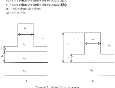
In this work, a rib structure was adopted for comparison as shown in Figure 2. From the figure, the labels are described as below:

n_s = substrate refractive index;

n_c = cladding refractive index;

n₂ = core refractive index for structure 2(a);

n₁ = core refractive index for structure 2(b);

n₃ = rib refractive index;

w = rib width.

Figure 2 (a) and (b) rib structures

n₁ t

d

n_s

n_c n_c

n3

n2

n_s w

h d

w

(b) (a)

3.1 Verification Test

Four rib waveguide structures with different parameters were simulated. The first structure was a COST structure [10], as depicted in Figure 2(a), in which the simulations

were done for three different values of rib height, particularly at t = 0.0, 0.2, and 0.4

µm. The other parameters were set to be constant where w = 2.4 µm and d = 0.2 µm.

The refractive index used were n_c = 1.0, n₁ = 3.17, n₂ = 3.38, and n_s = 3.17. This

structure has been used for years by many researchers to evaluate their methods [2, 8, 10]. We shall refer to this structure as structure A.

Simulations were also done for the rib structure as in Figure 2(b) with three different configurations which are listed in Table 1.

Waveguides in Table 1 were simulated and compared with works by researchers in [4, 5, 11]. Simulations were based on SOR value of 1.5 at 1.55 µm wavelength.

Table 1 Parameters of rib waveguide (Figure 2(b)) for comparison (n_c = 1.0)

Guide n₁ n_s n_c d(µµµµµm) h(µµµµµm) w(µµµµµm)

1 3.44 3.34 1.0 1.3 0.2 2

2 3.44 3.36 1.0 1.0 0.9 3

3 3.44 3.40 1.0 1.0 0.6-0.9 3

3.2 Performance Test

For evaluation purpose, simulations were divided into two distinct categories. The first category was to evaluate the effect of mesh size in producing the value of b with respect to number of iterations and computation time needed to complete the required task. The second category was to evaluate the effect of successive over relaxation (SOR) parameter in speeding up the iteration process while maintaining the mesh

size. Both simulations utilized the COST structure as in Figure 2(a) with t = 0.2 µm

and λ = 1.55 µm. For better comparison in the mesh sizes, we introduce the new

parameter of mesh ratio and defined as:

Mesh area Mesh ratio =

Structure area

where the structure area is defined as a box size with a value of 6 µm × 2.08 µm = 1.248

× 10–11 (µm)2 .

4.0 RESULTS AND DISCUSSION 4.1 Verification Test

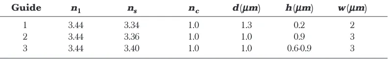
to work well if it is bounded by the value obtained using the effective index method (EIM), which sets the upper bound and the weighted index method (WIM) as the lower bound. The graphical plot of normalised propagation constant, b, for EIM, WIM and present finite difference (Present FD) is given in Figure 3 and it is strongly agreed to this bounded region. The contour plot of E field and refractive index distribution are shown in Figure 4.

Height of t in mikrometer

Normalized propagation constant

0.155 0.15 0.145 0.14 0.135 0.13 0.125 0.12 0.115

0 0.05

0.11

0.1 0.15 0.2 0.25 0.3 0.35 0.4

EIM WIM Present FD

Figure 3 Graphical plot of simulation result with a comparison to the EIM and WIM methods

Figure 4 Contour of E field and refractive index distribution for structure A

Y axis

Y axis x2.0e-8 m

60 50 40 30 20 10

20 60 80 100

0 _{X axis}

40

X axis x1.0 e-7 m

0 4 3 2 1

0

50 ₁₀₀ 150

Y axis 50 _{X axis}

0 4 3 2 1

0 50

E field

150 100

50 0

100

100

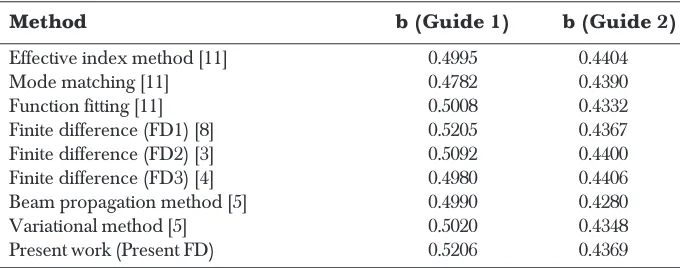
Table 2 and Figure 5 tabulate results for guide 1, 2 and 3 respectively. From Figure 5, results in this work are labelled as P-FD. Tabulated results show that the programmable finite difference method developed in this work is acceptable to be used for optical waveguide modelling purpose, due to small difference (up to only 5% difference) with other methods.

Table 2 Comparison of normalised propagation constant, b, for guide 1 and 2

Method b (Guide 1) b (Guide 2)

Effective index method [11] 0.4995 0.4404

Mode matching [11] 0.4782 0.4390

Function fitting [11] 0.5008 0.4332

Finite difference (FD1) [8] 0.5205 0.4367

Finite difference (FD2) [3] 0.5092 0.4400

Finite difference (FD3) [4] 0.4980 0.4406

Beam propagation method [5] 0.4990 0.4280

Variational method [5] 0.5020 0.4348

Present work (Present FD) 0.5206 0.4369

Normalized propagation constant (b

)

0.41 0.4 0.39 0.38 0.37 0.36 0.35 0.34 0.33

0.05 0.32

0.6 0.65 0.7 0.75 0.8 0.85

EIM VP VFEM SFEM SFDM P-FD

0.9 0.95

Guide thickness in micometer

4.2 Performance Test

(i) Simulation 1

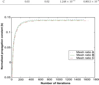
For the first simulation, three different mesh ratios were utilised as stated in Table 3. The performance of each mesh size in producing the normalised propagation constant, b, was evaluated with respect to number of iterations and computation time to complete the task. The results are depicted in Figures 6 and 7 respectively.

Table 3 Labelling of mesh sizes and respective mesh ratio

Mesh ∆x(µµµµµm) ∆y(µµµµµm) Box size(µµµµµm)2 Mesh ratio

A 0.2 0.02 1.248 × 10–11 3.2051 × 10–4 B 0.1 0.02 1.248 × 10–11 1.6025 × 10–4 C 0.05 0.02 1.248 × 10–11 0.8013 × 10–4

0 200 400 600 800 1000 1200 1400 1600 1800

0.05 0 0.05 0.1 0.15

Number of iterations

Mesh ratio A Mesh ratio B Mesh ratio C

According to the simulated data, the value of b converged to the value of 0.1435, 0.1408, and 0.1394 for mesh A, B, and C respectively. From this simulation, it clearly shows the effectiveness of reducing the mesh size, in which the value of b is more accurate but the drawbacks are increment in the required computation time. The phenomena can be explained by referring back to the Taylor series expansion. By increasing the mesh size, truncation error is increased, in which we have neglected the effect of higher order terms in the Taylor series expansion [7]. This truncation error can be reduced by decreasing the mesh size and iterations period [7]. Thus, less error is experienced by finer mesh size and it is more accurate in representing the differential functions.

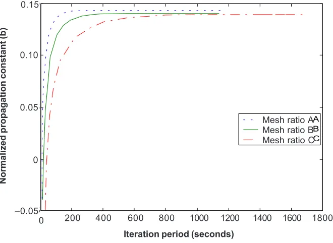
This phenomenon is in-line with our findings in which the fastest convergence was shown by mesh type A. It took almost 300 seconds approximately to converge while for mesh type B and C, 500 and 1100 seconds were needed respectively to fulfil the convergence task. The important thing that can be highlighted here is on the iterations number. For all the simulated mesh sizes, it took almost 700 iterations to converge. This is very important in our future work, in which the computer program can be initially set to iterate up to 700 iterations for all type of mesh sizes, as it proof to converge at this limit.

5 5 5

Mesh Ratio A Mesh Ratio B Mesh Ratio C

Normalized propagation constant (b)

0.15

0.10

–0.05 0.05

0

Iteration period (seconds)

0 200 400 600 800 1000 1200 1400 1600 1800 Mesh ratio A Mesh ratio B Mesh ratio C

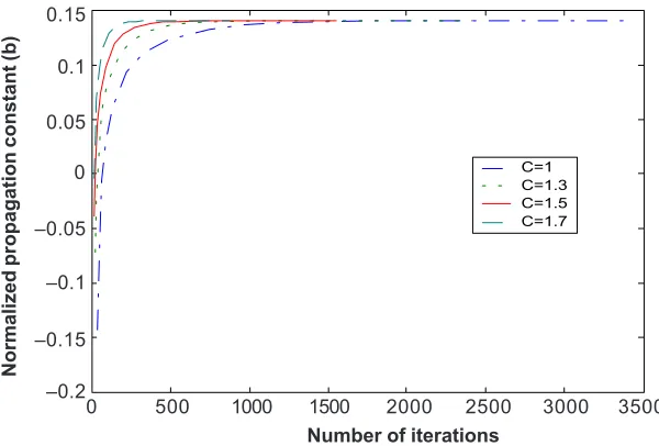
(ii) Simulation 2

To evaluate the effect of SOR parameter, the mesh size for the COST structure was chosen as type B for the reason of computation time and acceptable accuracy. Four different values of SOR were tested which are C=1 (without acceleration), C=1.3, C=1.5, and C=1.7. The results of b against the number of iterations and computation time are presented in Figures 8 and 9 respectively.

Figure 9 Graph of b against computation time for different Succesive Over Relaxation (SOR)

2 0

C=1 C=1.3 C=1.5 C=1.7

Normalised propagation constant (b)

0.15 0.1

–0.2 0.05 0

Computation time (seconds)

0 500 1000 1500 2000 2500 3000

–0.05 –0.1 –0.15

Figure 8 Graph of b against number of iterations for different Succesive Over Relaxation (SOR)

Normalized propagation constant (b)

0.15 0.1

–0.2 0.05 0

Number of iterations

0 500 1000 1500 2000 2500 3000 3500

C=1 C=1.3 C=1.5 C=1.7

From both figures, it shows that without acceleration, the convergence is very slow and it requires more iteration and computation time. As the SOR parameter increased, the convergence is faster and reduction in computation time is observed. However, if the SOR parameter is more than the tolerable value, the convergence is unstable [7, 9]. As a result, careful selection of SOR parameter is very important in future work as we need to balance between the accuracy requirement and computation hassle. From our

simulation, value of 1.3 ≤ C ≤ 1.7 is a good range to be utilised as it give shorter

computation time, while producing constant value of b.

5.0 CONCLUSION

The compatibility of the finite difference method for optical waveguide modelling purpose had been verified. The produced results portrayed its applicability as waveguide modelling tool. However, accumulation of truncation error during implementation will reduce its performance. Hence, the mesh size and the acceleration factor need to be chosen accordingly in order to get optimum design whilst reducing computation complexities.

ACKNOWLEDGEMENTS

The authors wish to thank the Ministry of Science, Technology and Innovation (MOSTI) for funding this research works under the National Top-Down Photonics Project. Our gratitude also goes to the members of Photonic Research Group (PRG) of Universiti Teknologi Malaysia for their help and fruitful discussions throughout the completion of this work.

REFERENCES

[1] Sharma, A., P. K. Mishra, and A. K. Ghatar. 1988. Single Mode Optical Waveguides and Directional Couplers with Rectangular Cross Section: A Simple and Accurate Method of Analysis. Journal of Lightwave Technology. 6(6): 1119-1125.

[2] Mohd Supa’at, A. S., A. B. Mohammad, N. Mohd Kassim, and R. Omar. 2002. Analysis of Mode Fields in Optical Waveguides. Proceedings of IEEE TENCON 2002. 2: 829-832.

[3] Benson, T. M., P. C. Kendall, M. S. Stern, and D. A. Quinney. 1989. New Results for Rib Waveguide Propagation Constants. IEE Proceedings. 136(2): 97-102.

[4] Stern, M. S. 1988. Semivectorial Polarised Finite Difference Method for Optical Waveguides with Arbitrary Index Profiles. IEE Proceedings. 135(1): 56-63.

[5] Weiping, H., and H. A. Hauss, 1991. A Simple Variational Approach to Optical Rib Waveguides. Journal of Lightwave Technology. 9(1): 56-61.

[6] Hayt, W. H., Jr, and J. A. Buck. 2001. Engineering Electromagnetics. 6th Edition. New York: McGraw-Hill International Edition.

[7] Sadiku, M. N. O. 2001. Numerical Techniques in Electromagnetics: Second Edition. Boca Raton: CRC Press LLC. [8] Mohd Kassim, N. 1991. Optical Waveguides in Silicon Materials. Ph.D. Thesis. University of Nottingham. [9] Booton, R. C., Jr. 1992. Computational Methods for Electromagnetics and Microwaves. New York: John Wiley

and Sons.

[10] Working Group 1, COST 216. 1989. Comparison of Different Modelling Techniques for Longitudinally Invariant Integrated Optical Waveguides. IEE Proceedings. 136(5): 273-280.