Comparison of COBRA-EN and COBRA-CTF Simulation Predictions to Benchmark Data for Representative Boiling Water Reactor Conditions.

(1)

MAULSTBY, JR., GREGORY ALLAN. Comparison of COBRA-EN and COBRA-CTF Simulation Predictions to Benchmark Data for Representative Boiling Water Reactor Conditions. (Under the direction of Dr. Joseph Michael Doster).

The purpose of this study is to compare predictions of two subchannel thermal-hydraulic codes,

COBRA-EN and COBRA-CTF, under representative boiling water reactor (BWR) operating

conditions with the steady-state, two-phase pressure drop benchmark data from the Nuclear

Power Engineering Corporation of Japan BWR Full-size Fine-mesh Bundle Test database.

Chapter two contains a brief description of the test facility used to conduct the experiments

along with the test assembly, grid spacers, and operating conditions and measured pressure

drop data for the test cases. Both COBRA-CTF and COBRA-EN sections include explanations

of input deck entries, methods to determine axial geometry, and unique differences and

challenges encountered. A mesh convergence study revealed that pressure predictions in both

thermal hydraulic codes were insensitive to the axial node length for a uniform node length of

0.1545m (0.50689ft) based on the given power profile. An additional study in COBRA-EN

determined two optimum combination of correlations based on pressure drop alone and another

that considers vapor fraction. The comparison of both codes to the benchmark data concluded

that COBRA-CTF requires further investigation of vapor fraction near the grid spacers, and

that both codes slightly under predict total pressure drop. In addition, COBRA-EN and

COBRA-CTF match the benchmark database well at most pressure drop identifiers but

measured vapor fraction is required to definitively claim which code predictions better

(2)

(3)

for Representative Boiling Water Reactor Conditions

by

Gregory Allan Maultsby Jr.

A thesis submitted to the Graduate Faculty of North Carolina State University

in partial fulfillment of the requirements for the degree of

Master of Science

Nuclear Engineering

Raleigh, North Carolina

2018

APPROVED BY:

______________________________ _______________________________

Dr. Maria Nikolova Avramova Dr. Stephen D Terry

(4)

BIOGRAPHY

Gregory Allan Maultsby, Jr. was born in Raleigh, North Carolina. He graduated high school in

1993 and returned to further his education in 2009. Received an Associate in Pre-Engineering in

2012 from Wake Technical Community College. Upon completion of the associate’s degree, he

transferred to North Carolina State University’s Nuclear Engineering program in the fall of

2012. After obtaining a bachelor in Nuclear Engineering in 2015, he stayed to pursue a Master

(5)

ACKNOWLEDGMENTS

“It takes a village to raise a child.”

-Unknown

By no far measure did I accomplish this master’s thesis alone. I would like to acknowledge the

following people for their contributions throughout this journey. First, I would like to thank

my graduate school advisor Dr. J. Michael Doster, of the Nuclear Engineering Department at

North Carolina State University for offering the opportunity to continue my education after my

undergraduate studies. He has continued to provide mentorship through his persistent patience

and guidance during the learning process of this master’s thesis. I would also like to

acknowledge Dr. Maria Avramova and Dr. Stephen Terry, as committee members. Also, I

would like to acknowledge Dr. Bourham, for taking time out of his schedule to attend my

defense as a committee member substitute. I received invaluable assistance from Dr. Taylor

Blythe for COBRA-CTF technical support, Dr. Robert Salko for general COBRA-CTF

support, and Dr. Konor Frick for his guidance and intellectually spirited discussions. I would

like to extend my appreciation for the funding support from CASL. Lastly, I would like to

acknowledge those who have contributed in a non-academic capacity. Sherry Bailey was a

consistent source of moral support throughout my experience in graduate school. We should

never forget those that wait for us while we chase our dreams. Ingrid Medina was a constant

source of stability in my life who always stood beside me for the full duration of my

(6)

TABLE OF CONTENTS

LIST OF TABLES ... vii

LIST OF FIGURES ... x

CHAPTER 1: Introduction ... 1

CHAPTER 2: NUPEC BFBT Benchmark ... 3

2.1 NUPEC Rod Bundle Test Loop ... 4

2.2 NUPEC BFBT High Burn-Up Assembly ... 6

2.3 Bundle Pressure Drop Locations ... 8

2.4 NUPEC BFBT C2A Power Profiles ... 10

2.5 NUPEC BFBT Grid Spacer ... 11

2.6 Subchannel Grid Spacer Loss Coefficients... 13

2.7 Representative BWR Operating Conditions ... 16

2.8 NUPEC BFBT Test Cases ... 19

CHAPTER 3: COBRA-CTF ... 21

3.1 Generalized Conservation Equations ... 24

3.2 Normal Wall Flow Regime Map ... 25

3.3 Pressure Drop ... 27

3.3.1 Friction Loss model ... 27

3.3.2 Form (Local) Loss Model ... 28

3.4 Water Properties... 28

3.5 Global Boundary Conditions ... 29

3.4.1 Inlet and Outlet Boundary Conditions ... 30

3.5 Convergence Study for COBRA-CTF ... 31

3.5.1 Methods for Mesh refinement ... 32

3.5.2 Base Mesh Refinement Technique ... 33

3.5.3 Uniform/Variable Mesh Refinement Technique ... 34

3.5.4 Mesh Refinement Cases ... 36

3.5.5 Adjustment to 5X24 ... 37

3.6 Total Power Forcing Function ... 47

3.6.1 Axial Power Profile... 48

(7)

3.7.1 P60001, Mesh Convergence Study Pressure and Vapor Fraction Plots ... 50

3.8 Mesh Convergence Study Analysis ... 53

3.8.1 Absolute Relative Differences for the Mesh Refinement Convergence Study ... 55

3.8.2 P60001, Axial Position Influence on Absolute Relative Differences ... 56

3.9 Convergence Study Conclusion ... 68

3.10 Axial Peaking Factors ... 70

3.11 Evaluation of the 1X24 and ETD Mesh Refinement Cases ... 73

3.11.1 P60001, Pressure and Vapor Fraction Plots of 1X24 and ETD Cases ... 74

3.11.4 P60015, Example of Differences in Pressure for 1X24 and ETD Cases ... 77

3.12 COBRA-CTF Results ... 80

CHAPTER 4: COBRA-EN ... 81

4.1 Subchannel Conservation Equations... 83

4.2 Subcooled Boiling Models ... 86

4.3 Void Quality Relations ... 88

4.4 Two Phase Friction Model ... 91

4.5 Pressure Drop ... 92

4.6 Water Properties... 94

4.7 COBRA-EN Axial Nodes ... 95

4.7.1 Description of the Normal Axial Nodes in COBRA-EN ... 97

4.7.2 Illustration of the Introduced Axial Nodes in COBRA-EN ... 98

4.8 Power Profile ... 100

4.9 COBRA-EN Boundary Conditions ... 102

4.9.1 Inlet Boundary Conditions ... 102

4.9.2 Outlet Boundary Conditions ... 103

4.10 Case Studies for COBRA-EN ... 103

4.10.1 Combination of Correlations for COBRA-EN ... 104

4.10.2 P60001, Evaluation of Total Pressure Drop ... 105

(8)

4.10.4 P60007 and P60015, Total Pressure Drop ... 108

4.10.5 P60007 and P60015, Pressure Drop for the Pressure Drop Identifiers ... 109

4.10.6 Result of the Correlations Study for Pressure Drop... 111

4.10.7 Further Evaluation of the Correlations Study ... 112

4.10.8 P60001, Plots for the Extended Correlations Study ... 114

4.10.9 P60007, Plots for the Extended Correlations Study ... 116

4.10.10 P60015, Plots for the Extended Correlations Study... 118

4.10.11 Results of the Extended Correlations Study ... 120

4.10.12 Conclusion of the Extended Correlations Study ... 122

4.11 Convergence Study with COBRA-EN... 123

4.12 Results of Convergence Study with COBRA-EN ... 124

CHAPTER 5: Comparison of COBRA-EN and COBRA-CTF ... 125

5.1 Comparison for Test Case P60001 ... 126

Conclusion and Future Work ... 135

REFERENCES ... 138

APPENDICES ... 139

Appendix A ... 140

Appendix B ... 142

Appendix C ... 143

Appendix D ... 146

Appendix E ... 155

Appendix F... 161

Appendix G ... 162

Appendix H ... 166

(9)

LIST OF TABLES

Table 2.1: Maximum Operating Conditions ... 4

Table 2.2: High Burn-up 8x8 Assembly ... 6

Table 2.3: Pressure Tap Axial Positions ... 9

Table 2.4: Length Between Pressure Tap Positions... 9

Table 2.5: Spacer Grid Locations ... 11

Table 2.6: ABWR and ESBWR Operating Conditions ... 17

Table 2.7: ABWR Operating Conditions ... 17

Table 2.8: Typical 8X8 BWR Operating Conditions... 18

Table 2.9: Selected Test Case Operating Conditions and Pressure Drop Measurements ... 19

Table 2.10: Range of NUPEC BFBT Test Parameters ... 20

Table 3.1: Total Inlet Mass Flow Rate... 29

Table 3.2: Average Linear Heat Rate per Rod ... 29

Table 3.3: Initial Guess for Pressure, PREF ... 30

Table 3.4: Inlet Fluid Temperature, TIN ... 30

Table 3.5: Mesh Refinement Case Uniform Node Length ... 36

Table 3.6: Test Case Mesh Refinement Technique Legend ... 36

Table 3.7: 5X24 Adjustment, Evaluation of 0.1mm Node Before 5th Grid Spacer ... 37

Table 3.8: 5X24 Adjustment, Change in Node Before 5th Grid Spacer ... 38

Table 3.9: 6X24 Adjustment, Evaluation of 0.75mm Node After 7th Grid Spacer ... 39

Table 3.10: 6X24 Adjustment, Change in Node After 7th Grid Spacer ... 39

Table 3.11: 7X24 Adjustment, Evaluation of 0.214mm Node Before 3rd_{Grid Spacer ... 40}

Table 3.12: 7X24 Adjustment, Change in Node Before 3rd Grid Spacer ... 40

Table 3.13: Further Adjustment to 7X24 Base Technique ... 41

Table 3.14: 7X24 Test 1, Evaluation of Node After 2nd Grid Spacer ... 42

Table 3.15: 7X24 Test 1, Change in Node After 2nd Grid Spacer ... 42

Table 3.16: 7X24 Test 1, Evaluation of Node After 7th_{Grid Spacer ... 43}

Table 3.17: 7X24 Test 1, Change in Node After 7th Grid Spacer ... 43

Table 3.18: Uniform/Variable Technique, 7X24 Test 6 and Test 8 ... 44

Table 3.19: Uniform/Variable Grid Spacer Padding for 7X24 Test 8 ... 45

Table 3.20: 8X24 Test 1 and Test 2 ... 46

Table 3.21: Powers with 0.3125 Extrapolated Axial Peaking Factor ... 48

Table 3.22: P60001 Absolute Relative Difference for 1X24 to 3X24 ... 54

(10)

Table 3.24: COBRA-CTF, P60001 Convergence Study Error Results for Void Fraction ... 57

Table 3.25: COBRA-CTF, P60001 Convergence Study Error Results for Flow Quality ... 58

Table 3.26: COBRA-CTF, P60007 Convergence Study Error Results for Pressure ... 60

Table 3.27: COBRA-CTF, P60007 Convergence Study Error Results for Vapor Fraction ... 61

Table 3.29: COBRA-CTF, P60015 Convergence Study Error Results for Pressure ... 64

Table 3.30: COBRA-CTF, P60015 Convergence Study Error Results for Vapor Fraction ... 65

Table 3.32: COBRA-CTF Center Points with Associated Axial Peaking Factors ... 71

Table 3.33: Measured Total Pressure Drop (psi) ... 73

Table 3.34: P60015, Smaller Node Size Between 5.577ft and 5.597ft in ETD Case ... 78

Table 3.35: P60015, Smaller Node Size Between 10.6463ft and 10.636ft in ETD Case ... 79

Table 3.36: COBRA-CTF Results for Pressure Drop ... 80

Table 4.1: COBRA-EN Node Edges ... 99

Table 4.2: COBRA-EN Thermal Output (MW) ... 100

Table 4.3: COBRA-EN Center Points ... 101

Table 4.4: Inlet Fluid Temperature, HIN ... 102

Table 4.5: Total Inlet Mass Flux Rate, GIN ... 102

Table 4.6: Exit Pressure, PEXIT ... 103

Table 4.7: Legend for Combinations of Correlations Used in COBRA-EN ... 104

Table 4.8: P60001 Evaluation for Total Pressure Drop of Measured Value 3.974 psi ... 105

Table 4.9: P60001 Absolute Relative Difference for Pressure Drop at Pressure Drop Identifiers ... 107

Table 4.12: P60007, Absolute Relative Difference for Pressure Drop at Pressure Drop Identifiers ... 110

Table 4.13: P60015, Absolute Relative Difference for Pressure Drop at Pressure Drop Identifiers ... 110

Table 4.14: COBRA-EN Results for Suite of Correlations, Set 8 ... 111

Table 4.15: P60001, Extended Combinations of Correlations Study ... 115

Table 4.18: P60001, COBRA-EN Extended Correlation Study Sets ... 120

(11)

Table 4.20: P60015, COBRA-EN Extended Correlation Study Sets ... 121

Table 4.21: COBRA-EN Results for Extended Set of Correlations, Set 1 ... 122

Table 4.22: COBRA-EN Convergence Study Uniform Node Lengths ... 123

Table 4.23: Results of COBRA-EN Convergence Study for Pressure (psi) ... 124

Table 5.1: P60001 COBRA-EN and COBRA-CTF Pressure Drop Comparison ... 126

Table 5.2: P60007 COBRA-EN and COBRA-CTF Pressure Drop Comparison ... 129

(12)

LIST OF FIGURES

Figure 2.1: System diagram of test facility for NUPEC rod bundle test series ... 5

Figure 2.2: Top-down view of the 8X8 high burn-up test bundle ... 7

Figure 2.3: Top left corner of 8X8 high burn-up test bundle... 7

Figure 2.4: Locations for pressure tap positions and pressure drop identifiers ... 8

Figure 2.5: Axial peaking factors in NUPAC BFBT C2A thermal profile ... 10

Figure 2.6: Radial peaking factors in NUPAC BFBT C2A thermal profile ... 10

Figure 2.7: Dimensions of ferrule type grid spacer (mm) ... 12

Figure 2.8: Legend of subchannel grid spacer loss coefficients ... 13

Figure 2.9: Typical diagram of a two-dimensional fuel channel ... 14

Figure 2.10: Grid spacer loss coefficients for top left corner ... 14

Figure 2.11: Grid spacer loss coefficients surrounding the central water channel ... 15

Figure 2.12: Average power/flow per bundle map for the ESBWR and BWR ... 16

Figure 3.1: COBRA-CTF normal wall flow regime map ... 26

Figure 3.2: Diagram of the Base mesh refinement technique ... 33

Figure 3.3: Diagram of the Uniform/Variable mesh refinement technique ... 35

Figure 3.4: Diagram of the padding in proximity of a grid spacer ... 35

Figure 3.5: Plot of failed solution convergence for P60001 5X24 with the 0.1mm node .... 37

Figure 3.6: Plot of solution convergence for P60001 5X24 without the 0.1mm node ... 38

Figure 3.7: Heat input over one fluid node ... 47

Figure 3.8: P60001, Pressure at axial positions for the convergence study mesh refinement cases ... 50

Figure 3.9: P60001, Vapor fraction at axial positions for the convergence study mesh refinement cases ... 50

Figure 3.14: P60001 Vapor fractions at shared axial position for all mesh refinement cases ... 59

Figure 3.15: P60007 Vapor fractions at shared axial position for all mesh refinement cases ... 63

(13)

Figure 3.17: Axial peaking factors for COBRA-CTF 1X24 and ETD compared to the

given values ... 72 Figure 3.18: P60001, Pressures of the COBRA-CTF 1X24 and ETD mesh

refinement cases ... 74 Figure 3.19: P60001, Vapor Fractions of the COBRA-CTF 1X24 and ETD mesh

refinement cases ... 74 Figure 3.20: P60007, Pressures of the COBRA-CTF 1X24 and ETD mesh

refinement cases ... 75 Figure 3.22: P60015, Pressures of the COBRA-CTF 1X24 and ETD mesh

refinement cases ... 76 Figure 3.24: Shift in pressure predictions observed in lower assembly positions for

1X24 and ETD cases ... 77 Figure 3.25: Shift in pressure predictions observed at 5.587ft and 7.27ft for 1X24 and

ETD cases ... 78 Figure 3.26: Shift in pressure predictions observed at 9.124ft, 10.646ft, and 11.57ft for

1X24 and ETD cases ... 79 Figure 4.1: Diagram of the lateral momentum control volume ... 85 Figure 4.2: Diagram to illustrate the construction of a normal COBRA-EN axial node ... 97 Figure 4.3: Diagram to illustrate the construction of an introduced COBRA-EN

axial node. ... 98 Figure 4.4: P60001, COBRA-EN EPRI suite’s vapor fraction predictions compared to

COBRA-CTF ... 114 Figure 4.5: P60001, Matched COBRA-EN sets compared to COBRA-CTF exit vapor

fraction predictions ... 114 Figure 4.6: P60001, Selected COBRA-EN sets compared to COBRA-CTF vapor

fraction trends ... 115 Figure 4.7: P60007, COBRA-EN EPRI suite’s vapor fraction predictions compared to

fraction trends ... 117 Figure 4.10: P60015, COBRA-EN EPRI suite’s vapor fraction predictions compared to

(14)

Figure 5.1: P60001, Pressure drop values at pressure tap identifiers ... 127

Figure 5.2: P60001, Percent difference in predicted to measured pressure drop ... 127

Figure 5.3: P60001, Pressure predictions of COBRA-CTF compared to COBRA-EN ... 128

Figure 5.4: P60001, Vapor fraction predictions of COBRA-CTF compared to COBRA-EN ... 128

Figure 5.5: P60007, Pressure drop values at pressure drop identifiers ... 130

Figure 5.8: P60007, Vapor fraction predictions of COBRA-CTF compared to COBRA-EN ... 131

Figure 5.9: P60015, Pressure drop values at pressure drop identifiers ... 133

(15)

CHAPTER 1: Introduction

The purpose of this study is to compare predictions of two subchannel thermal-hydraulic codes,

COBRA-EN and COBRA-CTF, under representative boiling water reactor (BWR) operating

conditions with benchmark data from the Nuclear Power Engineering Corporation (NUPEC)

of Japan BWR Full-size Fine-mesh Bundle Test (BFBT) database. This study is a continuation

of the ongoing validation and verification (V&V) process pertaining to the stand -alone

component, COBRA-CTF, in the code package VERA-CS sponsored by the Consortium for

Advanced Simulation of Lightwater Reactors (CASL). The primary validation metric for this

study is the steady-state, two-phase pressure drop benchmark from the NUPEC BFBT

database. Three of twenty-two test cases were selected to explore a variety of given parameters

such as thermal output, exit quality, total pressure drop, and mass flow.

First, it is important to understand the methods involved in collecting the measured benchmark

data in the NUPEC BFBT database. An electrically heated test loop was designed to simulate

a range of BWR operating conditions. Pressure drop measurements were taken at selected axial

positions along the heated bundle illustrated in figure 2.4 under operating conditions listed in

table 2.9. The BWR bundle design, axial and radial peaking factors, and grid spacer positions

are provided in the NUPEC BWR Full-size Fine-mesh Bundle Test (BFBT) Benchmark,

Volume I: Specifications [7]. The grid spacer local loss coefficients used in this study are

the same as used in previous CASL studies as represented in the, “CTF Validation and

(16)

For evaluation purposes, COBRA-EN and COBRA-CTF, are considered in separate sections.

These sections briefly describe the methods and models utilized in each code. In addition, there

are explanations of input deck entries, methods to determine axial geometry, and unique

differences and challenges encountered in each code. Furthermore, a mesh refinement study

was performed to determine the appropriate axial node length suitable for typical BWR

simulations. This supplementary study determines whether decreasing the axial mesh length

contributes to significant changes in code generated values at shared axial positions. The

default mesh length is based on the NUPEC BFBT database provided axial power peaking

factors illustrated in figure 2.5. These values are given for twenty-four uniform nodes of

lengths 154.5mm (0.50689ft) that sum to a total heated length of 3708mm (12.1654ft).

COBRA-CTF offers limited user options for choosing empirical closure relations as compared

to COBRA-EN. An additional study explores various combinations of two-phase correlations

and models in COBRA-EN to determine a best choice suite for comparison to the NUPEC

BFBT benchmark data. The “best choice suite” of correlations and models serves as the basis

(17)

CHAPTER 2: NUPEC BFBT Benchmark

The experimental data utilized for this study originates from the BFBT benchmark developed

by the NUPEC of Japan as a result of the fourth OECD/NRC BWR TT Benchmark Workshop

held on the sixth of October 2002 in Seoul, Korea [7].The NUPEC BFBT database addresses

concerns for nuclear applications to refine models for best estimate calculations based on good

quality experimental data [7]. Refer to NUPEC BWR Full-size Fine-mesh Bundle Test (BFBT)

Benchmark, Volume I: Specifications for the complete collection of the benchmark details and

exercises conducted. The primary focus for this study is the two-phase pressure drop, P6 series,

experiments located in the Phase II, “Critical Power Benchmark”, Exercise 0, “Steady State

Pressure Drop Benchmark. These experiments were conducted at the NUPEC BFBT facility

that can operate at the high pressure, and high fluid temperature conditions for typical reactor

(18)

2.1 NUPEC Rod Bundle Test Loop

Figure 2.1 illustrates the test loop used to conduct the NUPEC BFBT experiments. The structural

components are made of stainless steel (SUS304), and the cooling fluid is demineralized

water [7]. Electrically heated rod bundles are used to simulate a full scale BWR fuel

assembly [7]. The cladding, insulator, and heater were made of Inconel, boron nitride and

nichrome, respectively [7]. Mechanical properties listed in the appendix A are based on the

MATPRO model used in the TRAC code [7]. An adiabatic condition is suggested for the

benchmark considering no information on heat loss is available in the NUPEC BFBT

database [7]. The test loop can simulate a large range of steady-state BWR operating conditions.

Table 2.1 contains the maximum operating conditions for the BFBT test facility [7].

Table 2.1: Maximum Operating Conditions

Pressure Temperature Power Flow Rate

Metric

10.3 MPa 315 °C 12 MW 75 t/h

Standard

8.97 × 1013 𝑙𝑏𝑚

𝑓𝑡 ℎ𝑟2 599 °F 4.09 × 107

𝐵𝑇𝑈

ℎ𝑟 1.653 × 10

5 𝑙𝑏𝑚

(19)

A system diagram for the NUPEC rod bundle test series is illustrated in figure 2.1. A circulation

pump moves the coolant through three parallel control valves of different sizes to match the

desired flow rate for each case [7]. The fluid temperature entering the test section is controlled

by a direct-heating tubular pre-heater [7]. Sub-cooled coolant flows upward into the test section

where it is heated by the electrically heated rods to simulate the BWR operating conditions [7].

The coolant exiting the bundle is a mixture of steam and water that enters a separator where

the steam is separated and condensed using a sub-cooled water spray from two air-cooled heat

exchangers [7]. The condensed water is return to the circulation pump to complete the loop [7].

(20)

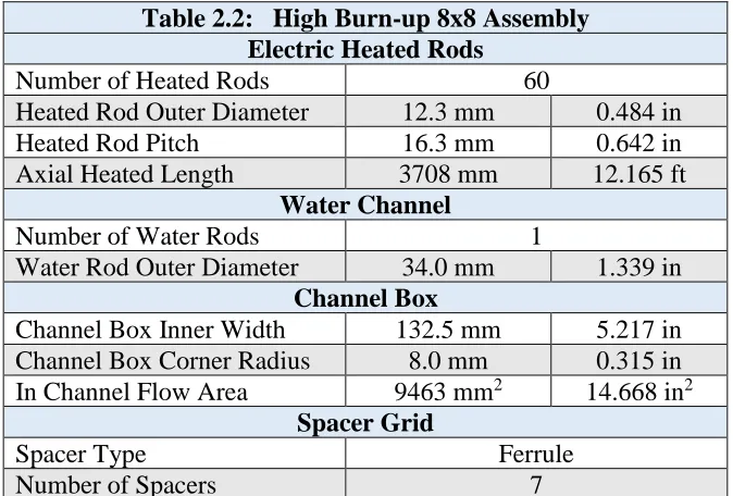
2.2 NUPEC BFBT High Burn-Up Assembly

The 8X8 High Burn-Up assembly is the chosen full-scale test bundle for this study. In addition,

the high burn-up assembly, classified as C2A, simulates beginning of operation radial peaking

conditions illustrated in figure 2.6 [7]. Table 2.2 list the number and dimensions of the heated

rods and water channels, the number of grid spacers, and the dimensions of the BWR

channel box [7].

Table 2.2: High Burn-up 8x8 Assembly Electric Heated Rods

Number of Heated Rods 60

Heated Rod Outer Diameter 12.3 mm 0.484 in

Heated Rod Pitch 16.3 mm 0.642 in

Axial Heated Length 3708 mm 12.165 ft

Water Channel

Number of Water Rods 1

Water Rod Outer Diameter 34.0 mm 1.339 in

Channel Box

Channel Box Inner Width 132.5 mm 5.217 in

Channel Box Corner Radius 8.0 mm 0.315 in

In Channel Flow Area 9463 mm2 14.668 in2

Spacer Grid

Spacer Type Ferrule

(21)

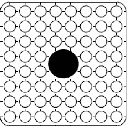
Figure 2.3 is a diagram of the top left corner with dimensions given in table 2.2.

0.642 in

0.484 in 0.315 in

Figure 2.2: Top-down view of the 8X8 high burn-up test bundle

(22)

2.3 Bundle Pressure Drop Locations

The bundle pressure drop was monitored at the locations indicated in Figure 2.4 [7].

(23)

Table 2.3 list seven pressure tap locations along the axial length of the test bundle where pressure

measurements were recorded. Both codes predict pressure at these positions that will be used to

determine the pressure drop at the nine pressure drop identifiers shown in figure 2.4.

Table 2.3: Pressure Tap Axial Positions Pressure Tap

Position Identifier

Axial Position (ft)

Axial Position (mm)

pt1 2.2375 682

pt2 5.5971 1706

pt3 7.2769 2218

pt4 8.9567 2730

pt5 9.7966 2986

pt6 10.6365 3242

pt7 11.4764 3498

Table 2.4 contains the nine pressure drop identifiers along with their associated lower and

upper axial positions, and spacing.

Table 2.4: Length Between Pressure Tap Positions Pressure Drop

Identifier

Lower Axial Position (ft)

Upper Axial

Position (ft) ΔZ (ft) ΔZ (mm)

dpt9 0.0 12.1654 12.1654 3708

dpt8 0.0 2.2375 2.2375 682

dpt7 2.2375 7.2769 5.0394 1536

dpt6 5.5971 7.2769 1.6798 512

dpt5 7.2769 8.9567 1.6798 512

dpt4 8.9567 10.6365 1.6798 512

dpt3 10.6365 12.1654 1.5289 466

dpt2 9.7966 10.6365 0.8399 256

(24)

2.4 NUPEC BFBT C2A Power Profiles

The axial power peaking factors are a cosine shape as shown in figure 2.5 [7].

The radial power profile for the beginning of operation (C2A) is illustrated in figure 2.6 [7].

1.15 1.30 1.15 1.30 1.30 1.15 1.30 1.15 1.30 0.45 0.89 0.89 0.89 0.45 1.15 1.30 1.15 0.89 0.89 0.89 0.89 0.89 0.45 1.15

1.30 0.89 0.89 0.89 0.89 1.15

1.15 0.45 0.89 0.89 0.89 0.89 0.45 1.15 1.30 1.15 0.45 0.89 0.89 0.45 1.15 1.30 1.15 1.30 1.30 1.15 1.15 1.15 1.30 1.15

Figure 2.5: Axial peaking factors in NUPAC BFBT C2A thermal profile

(25)

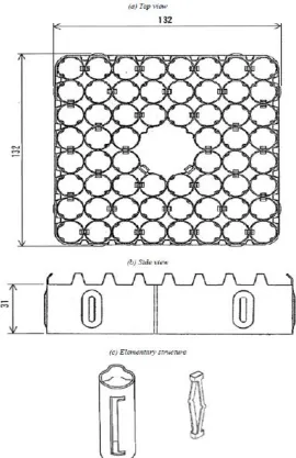
2.5 NUPEC BFBT Grid Spacer

Spacer grids provide structural support to the rod bundle during normal operation. Grid spacers

act as a local flow obstruction by means of decreasing the cross-sectional flow area resulting

in a local pressure drop. A ferrule type spacer is used in the NUPEC BFBT High Burn-Up

8X8 assembly experiments. These ferrule-type spacers contain circular tubes to guide each

heated rod as well as the central water rod [7]. Table 2.5 list the grid spacer positions along the

axial length of the heated rods [7].

Table 2.5: Spacer Grid Locations

(mm) (ft)

455 1.493

967 3.173

1479 4.852

1991 6.532

2503 8.212

3015 9.892

(26)

Figure 2.7 is an illustration of the ferrule-type grid spacer used during the NUPEC BFBT High

Burn-Up 8X8 assembly C2A experiments [7].

(27)

2.6 Subchannel Grid Spacer Loss Coefficients

For both COBRA-EN and COBRA-CTF, a local loss coefficient is supplied at user specified

axial position for each subchannel to model the impact of local flow obstructions due to grid

spacers. The approach in this study is to use the same loss coefficients as in CASL’s prior

evaluation of the NUPEC BFBT experiments illustrated in figure 2.8 [2]. These loss

coefficients were determined by B.S. Shiralkar and D.W. Radcliffe and reported in, “An

experimental and analytical study of the synthesis of grid spacer loss coefficients. Tech. rep.

NEDE-13181. General Electric, 1971” [2]. The loss coefficients identified in figure 2.8 have

not been independently verified in this study.

1.348 1.278 1.606 1.222 1.304 1.222 1.606 1.278 1.348

1.606 0.748 0.748 0.748 0.748 0.748 0.748 0.748 1.606

1.278 0.748 0.748 0.748 0.748 0.748 0.748 0.748 1.278

1.304 0.748 0.748 1.475 0.926 1.475 0.748 0.748 1.304

1.222 0.748 0.748 0.856 0.856 0.748 0.748 1.222

1.304 0.748 0.748 0.778 0.926 0.778 0.748 0.748 1.304

1.278 0.748 0.748 0.748 0.748 0.748 0.748 0.748 1.278

1.606 0.748 0.748 0.748 0.748 0.748 0.748 0.748 1.606

1.348 1.278 1.606 1.222 1.304 1.222 1.606 1.278 1.348

(28)

Figure 2.10 and figure 2.11 illustrate how the local loss coefficients for subchannels at the grid

spacer locations are defined as inputs to the codes. Figure 2.10 is the top left corner of the

bundle and represents a quarter of a fuel channel with a loss coefficient of 1.348, while along

the wall sides the sub-channels are half a fuel channel with respective loss coefficients of 1.278

and 1.606. The subchannel with the loss coefficient of 0.748 is a typical subchannel.

0.748 1.278

1.606 1.348

Figure 2.9: Typical diagram of a two-dimensional fuel channel

(29)

The large water channel in the center of the fuel assembly is treated as stagnant and not

associated with the mass flow of the bundle. The subchannel geometry and loss coefficients

surrounding the water channel are shown in figure 2.11.

1.475

0.856 0.856

1.475 0.926

0.926

0.778 0.778

(30)

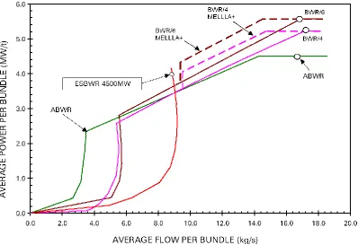
2.7 Representative BWR Operating Conditions

Figure 2.12 is an operaing power/flow map comparing the natural circulation ESBWR with

typical pump-driven BWRs currently in operation [9]. Figure 2.12 indicates that the typical

operating flow rate per bundle for currently operating BWRs is approximately 17kg/s while

the ESBWR is projected to operate near 9.0kg/s. In addition, the nominal average power per

bundle is approximately in a range between 3.8 to 5.8MWth for typical operating BWRs.

(31)

According to the IAEA website, https://aris.iaea.org/sites/core.html, table 2.6 is an additional

collection of typical operating conditions for the currently operating ABWR and the licensed

ESBWR [6].

Table 2.6: ABWR and ESBWR Operating Conditions Reactor

Type

Thermal Output

(MW)

Coolant Flow Rate

(kg/s)

Operating Pressure

(MPa)

Coolant inlet Temperature

(°C)

Number of Assemblies

ABWR 3926 14502 7.07 278 872

ESBWR 4500 9570 7.17 276.2 1132

Furthermore, the ABWR general design by General Electric reinforces the typical operating

conditions seen in table 2.7 [11].

Table 2.7: ABWR Operating Conditions Reactor

Type

Thermal Output

(MW)

(Mkg/hr)

(MPa)

Exit Quality %

Number of Rods per Assembly

ABWR 3926 52.2 7.17 14.5 872 92

The average bundle power and mass flow have been generalized in the following calculations

for comparison purposes to the test conditions in the NUPEC BFBT experiments.

ABWR average bundle power:

𝐴𝑣𝑒𝑟𝑎𝑔𝑒 𝐵𝑢𝑛𝑑𝑙𝑒 𝑃𝑜𝑤𝑒𝑟 = 3926𝑀𝑊

872 𝐵𝑢𝑛𝑑𝑙𝑒 = 4.502𝑀𝑊 𝑝𝑒𝑟 𝐵𝑢𝑛𝑑𝑙𝑒

ABWR average bundle mass flow:

𝐴𝑣𝑒𝑟𝑎𝑔𝑒 𝐵𝑢𝑛𝑑𝑙𝑒 𝑀𝑎𝑠𝑠 𝐹𝑙𝑜𝑤 = 14502

𝑘𝑔 𝑠

872 𝐵𝑢𝑛𝑑𝑙𝑒 = 16.63 𝑘𝑔

(32)

ESBWR average bundle power:

ESBWR average bundle mass flow:

𝑘𝑔 𝑠

1132 𝐵𝑢𝑛𝑑𝑙𝑒 = 8.45 𝑘𝑔

𝑠 𝑝𝑒𝑟 𝐵𝑢𝑛𝑑𝑙𝑒

These approximate values for the ABWR and ESBWR average bundle mass flow rates and

powers are based on 10X10 assemblies and are similar to values seen in figure 2.12. From “The Guide Book to Nuclear Reactors,” typical operating conditions for a pre-ABWR 8X8 are

seen given in table 2.8 [10].

Table 2.8: Typical 8X8 BWR Operating Conditions Thermal

Output (MW)

(Mg/s)

(MPa)

Exit Quality %

Number of Rods per Assembly

3579 13 7.0 14.7 748 62

BWR average bundle power:

BWR average bundle mass flow:

𝑀𝑔 𝑠

748 𝐵𝑢𝑛𝑑𝑙𝑒 = 17.38 𝑘𝑔

(33)

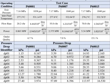
2.8 NUPEC BFBT Test Cases

The test cases P60001, P60007, and P60015 were selected to span a range of thermal

outputs, mass flows, and exit qualities. All three test cases exhibit the typical BWR exit

pressure of approximately 7.17MPa (1040psi). Test case P60015 approximates nominal

BWR operating conditions.

Table 2.9: Selected Test Case Operating Conditions and Pressure Drop Measurements Operating

Condition

Test Case

P60001 P60007 P60015

Exit

Pressure 7.16 MPa 1038 psi 7.17 MPa 1040 psi 7.17 MPa 1040 psi Inlet Fluid

Temperature 277.3°C 531.14°F 277.8°C 532.04°F 278.2°C 532.76°F Flow Rate 20.2 t/hr _4.44𝑋104 𝑙𝑏𝑚

ℎ𝑟 55.0 t/hr 1.21𝑋10 5 𝑙𝑏𝑚

ℎ𝑟 70.0 t/hr 1.54𝑋10 5 𝑙𝑏𝑚

ℎ𝑟

Power 0.863 MW 2.945𝑋106 𝐵𝑇𝑈

ℎ𝑟 2.375 MW 8.104𝑋10 6 𝐵𝑇𝑈

ℎ𝑟 5.34 MW 1.82𝑋10 7 𝐵𝑇𝑈

ℎ𝑟

Outlet

Quality 6.7 % 7.0 % 15.1 %

Pressure Drop Identifier

Pressure Drop

P60001 P60007 P60015

kPa psi kPa psi kPa psi

dp01 1.15 0.167 5.59 0.811 14.93 2.165

dp02 1.96 0.284 6.70 0.972 17.00 2.466

dp03 2.53 0.367 8.11 1.176 19.33 2.804

dp04 3.48 0.505 9.55 1.385 20.96 3.040

dp05 3.66 0.531 9.06 1.314 20.33 2.949

dp06 3.93 0.570 8.40 1.218 17.40 2.524

dp07 12.27 1.780 22.84 3.313 41.22 5.978

dp08 5.50 0.798 8.25 1.197 10.48 1.520

(34)

The full list of test case operating conditions and pressure drop measurements for the

P6 series experiments in the “Steady State Pressure Drop Benchmark” with the 8X8 High

Burn-Up test bundle, C2A, is in appendix B [7]. The range of given test parameters listed for

the NUPEC BFBT pressure drop experiment are given in table 2.10.

Table 2.10: Range of NUPEC BFBT Test Parameters

Flow Rate (t/h) Power (MW) Outlet Quality (%) Total Pressure Drop (kPa)

(35)

CHAPTER 3: COBRA-CTF

COBRA-TF was originally developed in 1980 by Pacific Northwest Laboratory under

sponsorship of the Nuclear Regulatory Commission (NRC) as a thermal hydraulic rod-bundle

analysis code [1]. COBRA-TF contributed toward goals set by revisions to NRC safety

analysis requirements (10 CFR.50.46) in 1988 to improve plant economy and safety with the

use of computational best-estimate models in plant design and operation [1]. COBRA-TF was

primarily designed to perform LWR rod-bundle transient analysis and simulate pressurized

water reactor (PWR) whole-vessel loss-of coolant accidents (LOCA) [1]. COBRA-CTF is an

improved version of COBRA-TF developed and maintained by the Reactor Dynamics and

Fuel Management Group (RDFMG) at the Pennsylvania State University (PSU) [1]. RDFMG

PSU improvements include [1]:

• Transition to FORTRAN 90 source code

• Enhanced user-friendliness with improved error checking and free-form input

• Quality assurance utilizing an extensive validation & verification (V&V) matrix

• Turbulent mixing, void drift and direct heating model improvements

• Enhanced computational efficiency by implementation of new numerical solution schemes

• Better code physical model and user modeling documentation.

As of August 2015, the RDFMG has been rebranded the Reactor Dynamics and Fuel Modeling

(36)

COBRA-CTF uses a two-fluid modeling approach involving three separate independent flow

fields which consist of a liquid film, liquid droplets, and vapor [1]. Each of the three fields

is modeled with its own set of conservation equations [1]. However, the liquid and droplet

flow fields are assumed to be in thermal equilibrium and share an energy equation [1]. The

user may choose how the sets of conservation equations are formulated either using a

Cartesian coordinate system or a subchannel approach [1]. A flow regime map based on a nodes’ current time step vapor fraction determines flow topology [1]. This allows for

determination of the interphase contact area, interphase heat transfer and drag, and the correct

selection of closure models [1].

The sub-channel approach is used for this study where only axial and lateral flows are

considered [1]. The lateral flow has no direction once it leaves a gap and applies to any

orthogonal direction to the vertical axis [1]. The COBRA-CTF Theory Manual states, “This is

a suitable assumption for the axially-dominated flow of a reactor fuel bundle because the

relatively minuscule lateral flows transfer little momentum across sub-channel mesh cell

elements [1].” The reason for choosing the simplified subchannel approach is that it utilizes

one less momentum equation for each of the three flow fields and is consistent with the

(37)

The equations are solved simultaneously using the Semi-Implicit Method for Pressure-Linked

Equations (SIMPLE) described in S.V. Patankar’s book, “Numerical Heat Transfer and

Fluid Flow [1].”

The steps of the SIMPLE algorithm are [1]:

1. Guess the pressure field, 𝑝∗.

2. Solve the momentum equations to obtain fluid velocities, 𝑢∗, 𝑣∗, and 𝑤∗.

3. Use the continuity equation to solve for the pressure field correction, 𝑝′_.

4. Calculate the corrected pressure field, p, by adding 𝑝′_to_𝑝∗_.

5. Calculate the corrected velocity field, u, v, and w, using the corrected pressure field.

6. Solve remaining discretized equations that influence the flow field.

7. Treat the corrected pressure, p, as the new guessed pressure, 𝑝∗_{and repeat steps 1-6}

until convergence is reached.

The SIMPLE method is explained in further detail in the COBRA-CTF theory manual. It is

important to take notice of the first step that mentions, “…the user must provide a reference

pressure... [1].” This guess for initial pressure is one of the inputs seen in Card 1, PREF, in

(38)

3.1 Generalized Conservation Equations

COBRA-CTF models each phase with its own set of mass, momentum, and energy equations [1].

The conservation equations for each flow field are linked by interaction terms that account for

mass, energy, and momentum transfer between phases [1]. The conservation equations are

discretized in space and time, and along with the appropriated closure relations, solved

numerically to provide estimates of the solution variables at fixed time intervals over mesh

cells representing the spatial domain [1]. There is a list of the parameters for the generalized

conservation equations in appendix C.

Generalized Phasic Mass Conservation Equation [1]: 𝜕

𝜕𝑡(𝛼𝑘𝜌𝑘) + ∇ ∙ (𝛼𝑘𝜌𝑘𝑉⃗ 𝑘) = 𝐿𝑘𝑀𝑒

𝑇₍₁₎

Generalized Phasic Momentum Conservation Equation [1]: 𝜕

𝜕𝑡(𝛼𝑘𝜌𝑘𝑉⃗ 𝑘) + 𝜕

𝜕𝑥(𝛼𝑘𝜌𝑘𝑢𝑘𝑉⃗ 𝑘) + 𝜕

𝜕𝑦(𝛼𝑘𝜌𝑘𝑣𝑘𝑉⃗ 𝑘) + 𝜕

𝜕𝑧(𝛼𝑘𝜌𝑘𝑤𝑘𝑉⃗ 𝑘) =

𝛼_𝑘𝜌_𝑘𝑔 − 𝛼_𝑘∇𝑃 + ∇ ∙ [𝛼_𝑘(𝜏_𝑘𝑖𝑗 + 𝑇_𝑘𝑖𝑗) + 𝑀⃗⃗ _𝑘𝐿+ 𝑀⃗⃗ _𝑘𝑑 + 𝑀⃗⃗ _𝑘𝑇]

(2)

Generalized Phasic Energy Conservation Equation [1]: 𝜕

𝜕𝑡(𝛼𝑘𝜌𝑘ℎ𝑘) + ∇ ∙ (𝛼𝑘𝜌𝑘ℎ𝑘𝑉⃗ 𝑘) = −∇ ∙ [𝛼𝑘(𝑄⃗ 𝑘+ 𝑞 𝑘

𝑇_{)] + Γ}

𝑘ℎ𝑘𝑖 + 𝑞𝑤𝑘′′′ + 𝛼𝑘

𝜕𝑃 𝜕𝑡 (3)

The subscript k denotes the phase:

𝑘 = {

(39)

3.2 Normal Wall Flow Regime Map

Flow regime maps are used to characterize the flow topology in each mesh cell [1]. This allows

for determination of the interphase contact area necessary for determination of interphase heat

transfer and drag, as well as the correct selection of flow regime dependent closure models [1].

The normal wall flow regime map is used when the maximum wall surface temperature in the

mesh cell described in equation 4 is below the critical heat flux temperature:

𝑇𝑊= 𝑚𝑖𝑛(705.3℉, 𝑇𝐶𝐻𝐹) (4)

where the upper limit of 705.3 °F corresponds to the critical temperature of water, and the

critical heat flux temperature is approximated by [1]:

𝑇_𝐶𝐻𝐹 = (𝑇_𝑆𝑎𝑡+ 75)℉ (5)

The hot wall flow regime map is used if the maximum wall temperature exceeds the value given

(40)

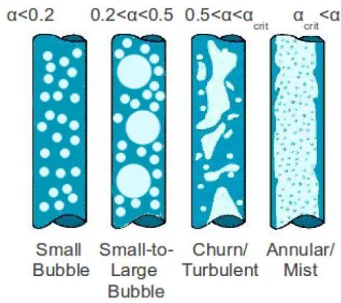
An initial void fraction check is made first to ensure that the mesh cell flow regime is consistent

with adjacent axial mesh cells. COBRA-CTF then selects the flow regime once the appropriate

void fraction is determined. Figure 3.1 illustrates the normal wall flow regimes with associated

vapor fraction ranges [1].

(41)

3.3 Pressure Drop

For more details on how pressure drop is managed in COBRA-CTF, refer to the Macro-Mesh

Cell Closure Models chapter in the COBRA-CTF theory manual [1].

3.3.1 Friction Loss model

COBRA-CTF uses a two-phase pressure drop model based on the work of Wallis [1]:

𝑑𝑃 𝑑𝑋)𝑓𝑟𝑖𝑐,𝑘

= 𝑓𝑤𝑘𝐺𝑘

2

2𝐷ℎ𝜌𝑘

Φ2 (6)

The frictional pressure drop term is calculated for both the vapor and liquid phase fields where

the mass flux of the field of interest is, 𝐺𝑘, and Φ2, is defined as [1]:

Φ2 = {1 𝛼₁⁄ 𝑙 𝑓𝑜𝑟 𝑛𝑜𝑟𝑚𝑎𝑙 𝑤𝑎𝑙𝑙 𝑐𝑜𝑛𝑑𝑖𝑡𝑖𝑜𝑛𝑠 𝛼_𝑣

⁄ 𝑓𝑜𝑟 ℎ𝑜𝑡 𝑤𝑎𝑙𝑙 𝑐𝑜𝑛𝑑𝑖𝑡𝑖𝑜𝑛𝑠 (7)

The phasic friction factor, 𝑓_𝑤𝑘, is defined using the phase Reynold’s number [1]. The

single-phase friction factor, 𝑓_𝑤𝑘, selected in the frictional pressure drop term has been used with prior

CASL evaluations of NUPEC BFBT two-phase pressure drop, P6 series, experiments for the Phase II, “Critical Power Benchmark”, Exercise 0, “Steady State Pressure Drop Benchmark.

𝑓_𝑤𝑘 = max {64 𝑅𝑒⁄ 𝑘 𝑙𝑎𝑚𝑖𝑛𝑎𝑟

0.204Re_𝑘−0.2 𝑡𝑢𝑟𝑏𝑢𝑙𝑒𝑛𝑡 (8)

Phase Reynolds number is based on phasic properties [1]:

𝑅𝑒_𝑘 =𝐷ℎ|𝐺𝑘|

(42)

3.3.2 Form (Local) Loss Model

The local pressure drop is defined as [1]: 𝑑𝑃

𝑑𝑋)𝑓𝑜𝑟𝑚,𝑘

= 𝛼𝑘

𝐾_𝑥

2Δ𝑋𝜌𝑘|𝑈𝑘|𝑈𝑘 (10)

The phase field, k, can be either liquid, vapor, or entrained droplets, and 𝑈𝑘 is the field velocity

[1]. The form loss coefficient, 𝐾_𝑥, may be user supplied, or code-calculated [1]. The grid spacer

loss coefficients labeled in figure 2.8 are the user supplied form loss coefficient, 𝐾_𝑥. COBRA-CTF

provides three methods to introduce local losses which include:

1. User specified loss coefficient provided at an axial location for a specified subchannel.

2. Calculate a flow blockage coefficient with a user specified pressure loss coefficient

multiplier and a user defined ratio of blocked area to flow area.

3. Grid spacer models explained in the COBRA-CTF theory manual.

This study only explored the first option as this is consistent with the method used by COBRA-EN

to manage local losses due to obstructions. This approach does not explicitly consider obstruction

type, geometry, or any other parameter other than its location and associated loss coefficient.

3.4 Water Properties

COBRA-CTF can calculate water properties such as thermal conductivity, specific heat,

viscosity, surface tension, and enthalpy for subcooled liquid, superheated vapor, and saturated

properties of both phases [1]. The International Association for the Properties of Water and

Steam (IAPWS) correlations to calculate the properties of water and steam have been

(43)

3.5 Global Boundary Conditions

The operating conditions are entered in Card 1.2, Global Boundary Conditions, for COBRA-CTF.

The total inlet mass flow rate is used to calculate subchannel mass flow rates for the user

specified subchannels flow areas [3].

Table 3.1: Total Inlet Mass Flow Rate

P60001 P60007 P60015

kg/s

5.611 15.278 19.444

lbm/s

12.370 33.682 42.868

t/hr

20.2 55.0 70.0

The average linear heat rate per rod is total bundle power divided by the total rod length

multiplied by the total number of rods [3]. This entry is used later to build power profiles.

Table 3.2 consist of the test cases’ value for with associated given thermal output.

𝑞_{̅ =}′ 𝑄

𝑁𝐻_{𝑓𝑢𝑒𝑙} (11) where:

𝑁 = Number of electrically heated rods (60)

𝐻_{𝑓𝑢𝑒𝑙}= Axial length of the electrically heated rod (3708mm or 12.165ft)

𝑄 = Total bundle thermal output

Table 3.2: Average Linear Heat Rate per Rod Test Case

P60001 P60007 P60015

Given Thermal Output (MW)

0.863 2.375 5.340

Average Linear Heat Rate per Rod (kW/m)

(44)

The initial guess for pressure in the fluid domain, PREF, for each test cases is listed in table 3.3.

Table 3.3: Initial Guess for Pressure, PREF

P60001 P60007 P60015

bar

71.6 71.7 71.7

MPa

7.16 7.17 7.17

psi

1038.4702 1039.9206 1039.9206

The user can either specify initial inlet enthalpy, HIN, or temperature, TIN, for the fluid

domain [3].

Table 3.4: Inlet Fluid Temperature, TIN

P60001 P60007 P60015

°C

277.3 277.8 278.2

°F

531.14 532.04 532.76

3.4.1 Inlet and Outlet Boundary Conditions

The inlet boundary conditions are total inlet mass flow rate used to calculate subchannel mass

flow rates for the user specified subchannels flow areas, and inlet fluid temperature, TIN. The

outlet boundary conditions are inlet fluid temperature, TIN, and exit pressure, PREF. The

COBRA-CTF user manual does provide the following disclaimer:

Note: The enthalpy specified at the exit is not used by COBRA-TF if flow is in the positive

direction (i.e. out of the model). In the case of positive flow, the user may enter any number

(45)

3.5 Convergence Study for COBRA-CTF

A mesh refinement (convergence) study was conducted to determine the sensitivity of

simulation results to axial node length. This was accomplished by establishing a uniform

mesh length based on the original data provided in figure 2.5. It is difficult to maintain a

true uniform axial mesh with COBRA-CTF as the local losses due to grid spacers require

their own identifying axial positions that interrupt this uniformity. This is not the situation

for COBRA-EN.

The specified uniform mesh length is propagated along the heated bundle until encountering

the non-uniform nodes before and after the grid spacer positions. Adjustments are made to

accommodate these varying size nodes in proximity of the grid spacer. Then, the uniform node

length would continue until it encountered the next grid spacer. This “Base” technique is a

viable option for a majority of the mesh refinement cases for the three test cases evaluated.

Modifications were required to ensure that some test cases would converge on a solution

with extra attention placed on nodes in proximity of the grid spacers. This modified technique labeled “Uniform/Variable” was required for the 7X24 and 8X24 mesh refinement cases with

the P60007 and P60015 test cases. In addition, the 5X24 mesh refinement case required a node

size of 0.1 mm to be absorbed into a previous node to achieve a converged solution. Lastly,

there was an exploration of relative size nodes in proximity of each other conducted in the

(46)

3.5.1 Methods for Mesh refinement

The methods chosen to conduct the mesh refinement convergence study for the three test cases

follow these constraints:

• Most importantly, achieve a converged solution with COBRA-CTF.

• Maintain the maximum number of uniform nodes possible while still providing grid

spacer identifiers.

• Attempt to maintain some uniformity between COBRA-EN and COBRA-CTF for

positions along the heated bundle to acquire data at the same locations.

• Maximize the number of axial positions shared between all the mesh refinement cases

to reduce the need to interpolate to determine a quantity of interest at a specific position.

This last criterion ensures that the values generated by COBRA-CTF are being evaluated at

common positions instead of introducing interpolation error. The primary quantities of interest

are pressure drops, considering that is the parameter being compared to in the NUPEC BFBT

benchmark database. There is also an evaluation of the vapor fraction, and flow quality. These

(47)

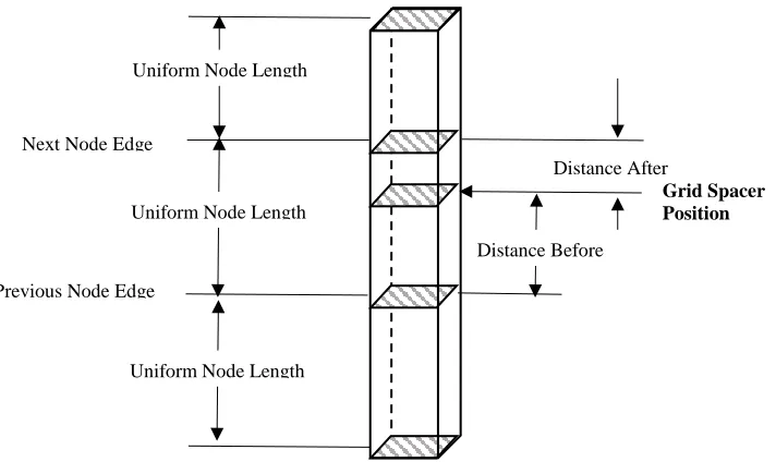
3.5.2 Base Mesh Refinement Technique

The distance before the grid spacer is determined by subtracting the upper edge of the previous

uniform node from the grid spacer position. The distance after the grid spacer is determined by

subtracting the grid spacer position from the lower edge of next uniform node. Figure 3.2

illustrates the Base technique applied near the grid spacer positions. It was observed that the

size of the nodes before and after the grid spacers pose issues with run time or inhibit a

converged solution. Furthermore, the run would converge faster and appear to be more stable

between each step if all node sizes are close to the same size as the surrounding nodes.

Grid Spacer Position

Next Node Edge

Previous Node Edge

Uniform Node Length

Uniform Node Length Uniform Node Length

Distance After

Distance Before

(48)

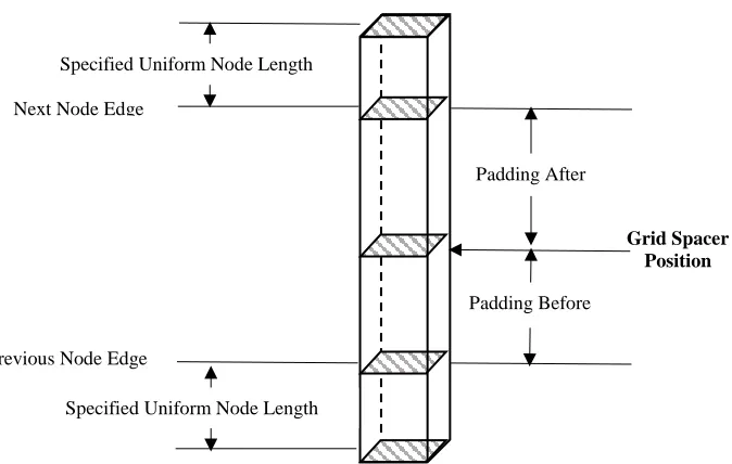
3.5.3 Uniform/Variable Mesh Refinement Technique

The Uniform/Variable (U/V) technique is a modified version of the Base technique built on

observations that nodes of the same size in proximity to each other affect the speed and stability

of reaching a converged solution. The variability introduced is due to the approximate uniform

mesh lengths specified for a mesh refinement case within the distances before and after the

grid spacers.

An arbitrary distance is determined by adding the previously calculated distance before the

grid spacer to a collection of uniform nodes. Then, this arbitrary distance is divided to provide

a node size that is approximately the same as the specified uniform node size. The same process

is repeated after the grid spacer. The specified uniform mesh size is reintroduced at the end of

the arbitrary distance after the grid spacer. Figure 3.3 illustrates the U/V technique at one grid

spacer. This process repeats for every grid spacer. This arbitrary distance before and after the grid spacer will be referred to as “padding.” Figure 3.4 illustrates this padding that contains a

collection of equal sized nodes that are approximately of the specified uniform node length.

The padding reduces the quantity of specified uniform node sizes and results in a reduction in

shared axial positions for the mesh refinement cases. Furthermore, this padding will introduce

(49)

Grid Spacer Position

Next Node Edge

Previous Node Edge

Specified Uniform Node Length

Padding After

Padding Before

Specified Uniform Node Length

Figure 3.4: Diagram of the padding in proximity of a grid spacer Figure 3.3: Diagram of the Uniform/Variable mesh refinement technique

Node Length of Approximate Uniform Node Length Size

“Padding” Stack of Nodes with Lengths

of Approximate Size of the Specified Uniform Node

(50)

3.5.4 Mesh Refinement Cases

The mesh refinement cases are categorized by the number of times the original node size seen

in figure 2.5 is sub-divided.

𝑈𝑛𝑖𝑓𝑜𝑟𝑚 𝑁𝑜𝑑𝑒 𝐿𝑒𝑛𝑔𝑡ℎ = 𝐻𝑓𝑢𝑒𝑙

𝐷𝑁 (12)

𝐻_{𝑓𝑢𝑒𝑙}= Axial length of the electrically heated rod

𝐷 = Number divisions per node

𝑁 = Number original nodes

Table 3.5: Mesh Refinement Case Uniform Node Length Mesh Refinement Case

1X24 3X24 4X24 5X24 6X24 7X24 8X24

Uniform Node Length Metric (m)

0.1545 0.0515 0.038625 0.0309 0.02575 0.02207 0.0193125

Standard (in)

6.08268 2.02756 1.52067 1.21654 1.01378 0.86895 0.76033

* Bold indicates approximates values

Table 3.6 reflects the mesh refinement technique used to produce the results for each test case

for each mesh refinement case.

Table 3.6: Test Case Mesh Refinement Technique Legend

Test Case Mesh Refinement Case

1X24 3X24 4X24 5X24 6X24 7X24 8X24

P60001 Base Base Base *Base *Base *Base Base

P60007 Base Base Base *Base *Base *Base U/V

P60015 Base Base Base *Base *Base U/V U/V

(51)

3.5.5 Adjustment to 5X24

Applying the Base technique results in the spaces before and after the fifth grid spacer seen in

table 3.7. The axial positions are defined by the node edges. Axial position 2.503m, is the fifth

grid spacer position while 2.472m and 2.5338m are axial positions shared by all the mesh

refinement cases.

Table 3.7: 5X24 Adjustment, Evaluation of 0.1mm Node Before 5th_{Grid Spacer} Node Length (m)

Uniform Node

Previous Uniform Node

Before Grid Spacer

After Grid Spacer

Next Uniform Node

0.0309 0.0309 0.0001 0.0308 0.0309 0.0309

Axial Position (m)

2.472 2.5029 2.503 2.5338 2.5647

Figures 3.5 and 3.6 are plots of the time steps versus percent total energy storage for both

techniques for mesh refinement case 5X24. Figure 3.5 illustrates that after 40,000 steps the

solution does not appear to be reaching convergence after a force quit was applied. This may

reach a converged solution, but it would have taken excessive run times.

0 100 200 300 400 500 600 700 800 900 1000

0 5000 10000 15000 20000 25000 30000 35000 40000

%

T

o

ta

l En

er

g

y

Sto

ra

g

e

Time Steps

(52)

A solution was obtained once the 0.1mm before the grid spacer is adjusted. Table 3.8 reflects

that the 0.1mm space was absorbed in the next uniform space after the 2.472m position.

This preserves the positions of interest, 2.472m, 2.503m, and 2.5338m. in addition, all the

nodes in this area are approximately the same size. This correction allows for the run to

converge on a solution.

2.472𝑚 + 0.031𝑚 = 2.503𝑚

Table 3.8: 5X24 Adjustment, Change in Node Before 5th_{Grid Spacer} Node Length (m)

0.0309 0.0309 0.031 0.0309 0.0309 0.0309

2.4411 2.472 2.503 2.5338 2.5647

Figure 3.6 illustrates that the solution is achieved at 4610 steps.

0 100 200 300 400 500 600 700 800 900 1000

0 1000 2000 3000 4000 5000

%

T

o

ta

l En

er

g

y

Sto

ra

g

e

Time Steps

(53)

Applying the Base technique results in the space before and after the seventh grid spacer seen

in table 3.9. Axial position, 3.527m, is the seventh grid spacer position while 3.5535m is an

axial position shared by all the mesh refinement cases.

Table 3.9: 6X24 Adjustment, Evaluation of 0.75mm Node After 7th_{Grid Spacer} Node Length (m)

0.02575 0.02575 0.025 0.00075 0.02575 0.02575

2.47625 3.502 3.527 3.52775 3.5535

Table 3.10 shows that the 0.75mm space is absorbed with the following uniform distance

starting at 3.52775m. This preserves the positions of interest 3.527m, and 3.5535m. in addition,

all the nodes in this area are approximately the same size. All three test cases can use both

methods to converge on a solution.

Table 3.10: 6X24 Adjustment, Change in Node After 7th_{Grid Spacer} Node Length (m)

0.02575 0.02575 0.025 0.0265 0.02575 0.02575

3.47625 3.502 3.527 3.5535 3.57925

Including the 0.75mm after the grid spacer, the run for P60001 takes 24,810 steps to reach a

converged solution. When the distance of 0.75mm is absorbed, the solution converges after

(54)

Applying the Base technique to P60001 test case results in the space before and after the third

grid spacer seen in table 3.11. Axial position, 1.479m, is the third grid spacer position. The

uniform mesh size of approximately 0.022071m, allows for four nodes before and one node

after the two spaces surrounding the grid spacer which results in the two axial positions shared

by all the mesh refinement cases, 1.3905m and 1.545m respectively.

Table 3.11: 7X24 Adjustment, Evaluation of 0.214mm Node Before 3rd_{Grid Spacer} Node Length (m)

0.022071 0.022071 0.000214 0.021857 0.022071 0.022071

1.4567 1.4788 1.479 1.50086 1.5229

Table 3.12 shows that the 0.214mm space is absorbed with the previous uniform distance

starting at 1.4567m. This preserves the grid spacer position 1.479m. In addition, all the nodes

in this area are approximately the same size.

Table 3.12: 7X24 Adjustment, Change in Node Before 3rd_{Grid Spacer} Node Length (m)

0.022071 0.022071 0.022286 0.021857 0.022071 0.022071

1.4346 1.4567 1.479 1.50086 1.5229

The same acceleration is observed as the mesh refinement case 6X24. Including the 0.214mm

after the grid spacer, the run for P60001 takes 56,632 steps to reach a converged solution. The

(55)

The Base technique used in the P60001 test case did not converge on a solution and exhibited an

oscillatory behavior for P60007 until a user force quit applied at 80,000 steps. This lead to more

adjustments to the Base technique labeled “Test 1” where further attempts to ensure node lengths

are more similar in size to nodes in proximity. Table 3.13 reflects the location of further

adjustments made compared to the Base technique for the 7X24 mesh refinement case labeled “With 0.241mm.” The locations marked in bold red indicate quantity of nodes, JLEV, with node

lengths, VARDX, prior to adjustments while the bold black text marks the adjustments. Further adjustments to the 7x24 mesh refinement case labeled “Test 1” include modifications to node

lengths near the second and seventh grid spacer.

Table 3.13: Further Adjustment to 7X24 Base Technique

With 0.214mm Without 0.214mm 7X24 Test 1

JLEV VARDX JLEV VARDX JLEV VARDX

No Change

46 0.017928571429 46 0.017928571429 46 0.017928571429

47 0.004142857143 47 0.004142857143 47 0.026214285714

70 0.022071428571 69 0.022071428571 68 0.022071428571

71 0.000214285714 70 0.022285714286 69 0.022285714286

72 0.021857142857 71 0.021857142857 70 0.021857142857

No Change

167 0.017642857143 166 0.017642857143 165 0.017642857143