Construction of C^2 Q^5 and C^2 Q^7 Finite Elements on 2D Rectangular Meshes

ABSTRACT

YU, FEI. Construction ofC2Q5 and C2Q7 Finite Elements on 2D Rectangular Meshes. (Under the direction of Dr. Zhilin Li).

Finite element method is one of the most powerful and commonly used numerical

meth-ods in almost everywhere in mathematics. Finite elements with certain continuity are also

becoming more and more popular, for example, splines for 1D interpolation. However, there

Construction of

C

Q

and

C

Q

Finite Elements on 2D Rectangular

Meshes

by

Fei Yu

A thesis submitted to the Graduate Faculty of

North Carolina State University

in partial fulfillment of the

requirements of the degree of

Master of Arts

Mathematics

Raleigh, North Carolina

2012

APPROVED BY:

Ernest Stitzinger

Xiaobiao Lin

Zhilin Li

BIOGRAPHY

Fei Yu was born in the northeast of China. He entered Harbin Institute of

Technol-ogy(HIT) in 2007, majoring Computer Science. After three years’ study in HIT, he went

to University of Birmingham in England for a 3+1 program and got Bachelor Degrees from

both HIT and University of Birmingham in 2011. Now he is a master student of North

Car-olina State University, majoring in Mathematics. His reseach focuses on numerical analysis

ACKNOWLEDGEMENTS

I would like to thank my advisor Dr. Zhilin Li for his supervision and helpful suggestions

TABLE OF CONTENTS

LIST OF TABLES... v

LIST OF FIGURES... vi

1. Introduction... 1

2. C2Q5 finite elements on 2D rectangles... 3

2.1. Construction of C2Q5 finite elements... 3

2.2. A numerical experiment on C2_Q5 _{finite elements... 6}

3. C2Q7finite elements on 2D rectangles... 10

3.1. Construction of C2Q7 finite elements... 10

3.2. A numerical experiment onC2_Q7 _{finite elements... 11}

4. A numerical test onC2Q5interpolation... 13

5. Conclusions and future work... 17

LIST OF TABLES

Table 1 Errors×10−10of C2Q5 in infinity norm alongx= 0... 8

Table 2 Errors×10−10 ofC2Q5 in infinity norm alongy= 0... 8

Table 3 Errors×10−10ofC2Q7 in infinity norm alongx= 0... 13

Table 4 Errors×10−10ofC2Q7 in infinity norm alongy= 0... 13

LIST OF FIGURES

Figure 1 Quadrilateral mesh... 2

Figure 2 Two neighbor squares (part of figure 1)... 2

Figure 3 A small square after partition... 4

Figure 4 Mesh for shape function... 6

Figure 5 PlotQ5 forC2Q5 with onlyu= 1 at center point... 9

Figure 6 PlotQ5_x forC2Q5 with onlyu= 1 at center point... 9

Figure 7 PlotQ5_y forC2Q5 with onlyu= 1 at center point... 9

Figure 8 Plot Q5 xx forC2Q5 with only u= 1 at center point... 9

Figure 9 Plot Q5_xy forC2Q5 with only u= 1 at center point... 9

Figure 10 PlotQ5_yy forC2Q5 with onlyu= 1 at center point... 9

Figure 11 PlotQ7 _forC2_Q7 _{with onlyu= 1 at center point... 12}

Figure 12 Plot Q7_x forC2Q7 with only u= 1 at center point... 12

Figure 13 Plot Q7_y forC2Q7 with only u= 1 at center point... 12

Figure 14 PlotQ7 xx forC2Q7 with only u= 1 at center point... 12

Figure 15 PlotQ7_xy forC2Q7 with onlyu= 1 at center point... 12

Figure 16 PlotQ7_yy forC2Q7 with onlyu= 1 at center point... 12

Figure 17 Error ofC2_Q5 _{interpolation foru= sin(πx) sin(πy) withh= 1... 16}

Figure 18 Error ofC2Q5 interpolation for u= sin(πx) sin(πy) withh= 1/2... 16

Figure 19 Error ofC2Q5 interpolation for u= sin(πx) sin(πy) withh= 1/4... 16

Figure 20 Error ofC2Q5 interpolation foru= sin(πx) sin(πy) withh= 1/8... 16

Figure 21 Error ofC2Q5 interpolation foru= sin(πx) sin(πy) withh= 1/16... 16

1

Introduction

In the mathematical field of numerical analysis, finite element method always plays a very

important role by providing a numerical technique for finding approximate solutions to

partial differential equations (PDE) and their systems, as well as integral equations [1].

Finite element method is widely used and lots of researches have been done since its

invention [2,3]. Then mathematicians started to look at special finite element spaces with

certain continuity. For one-dimension, splines, especially cubic splines, are commonly

ap-plied to a variety of problems. For instance, In [4], the author described the use of cubic

splines for interpolating monotonic data sets, In [5], a way to construct shape-preserving

C2 cubic polynomial splines interpolating convex and/or monotonic data was developed. Also, there was a C2 interpolation using quartic splines in [6]. However, when it comes to two-dimension, finite elements that are continuously differentiable are relatively difficult to

build [7]. Some researches have been done to contruct these C1 elements on triangles by using polynomialPkorQk, wherePkandQkrepresent polynomials of total degree and sep-arate degree k respectively. For example, the Powell-Sabin P2-triangle [8] and the Argyris P5-triangle [9]. As to rectangles, the Boger-Fox-Schmit rectangle [10] is the most famous and commonly used one in C1. Also, in [7], the author extended the Bogner-Fox-Schmit element toC1Qk in 2D and 3D, k≥3.

In fact, there are quite few papers focusing on C2 finite elements on 2D rectangles. Nevertheless, some important applications of C2 _{finite elements cannot be neglected. For} example, these finite elements can be used to solve the fourth order (or even higher) PDEs,

like biharmonic equation. Also, Peskin’s Immersed Boundary (IB) method [11], which is one

to prove the convergence order of the IB method, we need to find an interpolate function

to interpolate the discrete delta functions. Such an interpolation function can be obtained

from the C2 finite element spaces we introduce in this thesis. We consider the following problem:

Given a quadrilateral mesh (squares), for instance, figure 1, can we find the minimumk such that the piecewise bipolynomial interpolation

Qk(x, y) =

i≤k,j≤k

X

i=0,j=0 cijxiyj

has the following properties:

(a) Qk(x, y)∈C2; (b)Dα_(x

m, yn),0≤ kαk1 ≤2(or 3) are given, that is, the function values, and up to all the second (or third) order partial derivatives are given at (xm, yn).

Figure 1: Quadrilateral mesh

x=a

Figure 2: Two neighbor squares (part of figure 1)

Two neighbor squares of the whole mesh are shown in figure 2. In each square, since the

how to maintain the continuity along the boundary, for example, the intersection x =a of the two neighbor squares, as shown in figure 2. In order to get theC2 finite element spaces, we need the function values and all up to the second order derivatives, which are :

Qk, Qk_x, Qk_y, Qk_xx, Qk_xy, Qk_yy, whereQkis the interpolation function andQk_xstands for ∂Q_∂xk. to be continuous along the 4 sides of each square.

In this thesis, we develop two finite elements,C2Q5 andC2Q7, that belong toC2 for 2D rectangles. In section 2, we consider that at each nodal point of the rectangle, up to second

order partial derivatives are given and we construct bipolynomials Q5 that belongs toC2. In section 3, we consider that at each nodal point of the rectangle, up to third order partial

derivatives are given and we construct bipolynomialsQ7 _{that belongs toC}2_{. In section 4, we} run a numerical interpolation test on u= sin(x) sin(y) using C2Q5 finite elements. Finally in section 5, we introduce some possible applications of these C2 finite element spaces.

2

C

2

Q

5

finite elements on 2D rectangles

2.1

Construction of

C

Q

finite elements

In this section, we discuss the construction of C2Q5 finite elements on 2D rectangles. We consider the problem discussed in section 1 when the function values and all up to the second

order derivatives are given at each nodal point.

Let Ω be a rectangle domain in 2D. For simplicity, we may let Ω be the unit square with

the uniform grid of size. Then after partition we can arbitrarily take one small square,[a, b]×

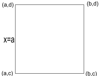
[c, d](d-c=b-a), as an example as shown in figure 3.

For each point of the square, we already have 6 values, the function values and all up to

the second order derivatives. However, in order to get the continuities along the boundaries,

(a,d)

(a,c) (b,c)

(b,d)

x=a

Figure 3: A small square after partition

9 values for the 4 points of a square. The total constrains are 4×9 = 36, which is exactly

the same as the degree of freedom (DOF) of the bipolynomial Q5. So let k be 5 and now we prove that the interpolation functionQ5 we get indeed belongs to C2.

First, we introduce a theorem and prove it.

Theorem 2.1. LetQkbe a bipolynomial interpolation function with separate degreekon a quadrilateral mesh (in figure 1). For two neighbor squares (in figure 2)Qk has continuous second order derivatives along the boundaryx=a(ory=b) ifQk|_x=a, Qk_x|_x=aandQk_xx|_x=a (or Qk|_y=b, Qk_y|_y=b andQk_yy|_y=b) are all continuous, wherea, b are constant.

Proof: We only need to prove the case when the boundary isx=aas shown in figure 2, since the proof is similar for y=bcase.

Since Qk|x=a is continuous, the function value is continuous along x = a. Meanwhile,

all the tangential (or Y) direction derivatives ∂_∂ynQnk, n ≥ 1 are also continuous along this

boundary, this is because we can conclude the continuity of ∂nQk|x=a

∂yn from the continuity of Qk|x=a and

∂n_Qk_| x=a

∂yn =

∂n_Qk

∂yn |x=a

Here, we only use the continuities of up to second order derivatives, which are Qk_y|_x=a

Similarly, since Qk_x|x=a is continuous, Qkx and Qkxy are continuous along the boundary.

At last, we also have the continuity of Qk_xx along x=a.

Thus, the function value and up to second order derivatives of Qk are all continuous along the boundaryx=a. This completes the proof of Theorem 2.1.

Remark 2.2. If for any two neighbor squares in the whole mesh, Qk always has con-tinuous second order derivatives along the boundary, then Qk ∈C2.

Then we use the theroem to prove that the interpolation function Q5 _{we get indeed} belongs to C2.

Along one side, for instancex=a,Q5|x=ais a fifth polynomial ofy, which has the form:

Q5_|

x=a=β5y5+β4y4+β3y3+β2y2+β1y+β0

Clearly, the DOF of Q5|_x=a is 6. We have the values of u, uy, uyy at both nodal points,

(a, c) and (a, d), which form 6 equations to uniquely determineQ5|x=a.

Then, we take a look at Q5_x|_x=a, it is also a fifth polynomial ofy, which has the similar form asQ5|_x=adoes. It is uniquely determined by the values ofux, uxy, uxyy at both points.

At last, as to Q5_xx|x=a, which is still a fifth polynomial of y, we have the values ofuxx

uxxy anduxxyy at two points, which are used to uniquely determine Q5xx|x=a.

So far, Q5|x=a,Q5x|x=a and Q5xx|x=a are all continuous. According to Theorem 2.1, we

have obtained up to the second order continuity along x= a. In fact, the proof is similar for the other side, x =b. Meanwhile, the other two sides, y =c and y =d, are also taken care of. For example, alongy=c:

• The values of u, ux and uxx at both points, (a, c) and (b, c), uniquely determine the

fifth polynomial Q5|_y=c.

Q5_y|y=c.

• The values ofuyy, uxyy anduxxyy at both points uniquely determine the fifth

polyno-mialQ5_yy|y=c.

Hence, along each of the 4 sides, the interpolation function Q5 always has continuous second order derivatives along the boundary. Since we choose the square arbitrarily,

ac-cording to Remark 2.2, the interpolation function Q5 indeed belongs to C2. We have a system of equations with 36 unknowns and 36 equations. The rank of the coefficient matrix

that matlab returns is 36, which indicates that the matrix is non-singular and the system

of equations has a unique solution.

2.2

A numerical experiment on

C

Q

finite elements

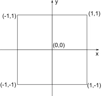
Now, we consider 2D square, [−1,1]×[−1,1], as an example. We partition it into 4 squares, [−1,0]×[0,1], [0,1]×[0,1], [−1,0]×[−1,0] and [0,1]×[−1,0] as shown in figure 4.

(-1,1)

(0,0)

(1,1)

(1,-1) (-1,-1)

y

x

Figure 4: Mesh for shape function

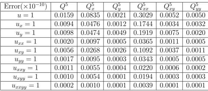
functionQ5, which are obtained by imposing function value u of the center point,(0,0), to be 1 and all the rest to be 0. Also, in table 1-2, we calculate the errors in the infinity norm

for up to all the second order derivatives along the boundariesx= 0 andy= 0 respectively by taking the absolute values of the differences between the values of two sides. Also, each

row of the tables indicates that one of the 9 values (all up to the second order derivatives

and uxxy, uxyy, uxxyy) of the center point is imposed to be 1 and the rest are all 0.

According to the figures of plots and the tables of errors, we can also conclude that the

Table 1: Errors(×10−10) of C2Q5 in infinity norm along x= 0

Error(×10−10_{) Q}5 _Q5

x Q5y Q5xx Q5xy Q5yy

u= 1 0.0051 0.0738 0.0146 0.0053 0.1376 0.0470

ux = 1 0.0008 0.0403 0.0035 0.0024 0.0737 0.0161

uy = 1 0.0031 0.0399 0.0083 0.0027 0.0743 0.0248

uxx = 1 0.0004 0.0079 0.0010 0.0005 0.0150 0.0037

uxy = 1 0.0005 0.0217 0.0018 0.0012 0.0395 0.0077

uyy = 1 0.0005 0.0080 0.0017 0.0006 0.0150 0.0050

uxxy= 1 0.0002 0.0042 0.0006 0.0003 0.0080 0.0020

uxyy = 1 0.0001 0.0044 0.0005 0.0002 0.0080 0.0020

uxxyy = 1 0.0001 0.0008 0.0001 0.0001 0.0016 0.0003

Table 2: Errors(×10−10_{) of C}2_Q5 _{in infinity norm along y= 0}

Error(×10−10_{) Q}5 _Q5

x Q5y Q5xx Q5xy Q5yy

u= 1 0.0159 0.0835 0.0021 0.3029 0.0052 0.0050

ux = 1 0.0094 0.0476 0.0012 0.1744 0.0034 0.0032

uy = 1 0.0098 0.0474 0.0049 0.1919 0.0075 0.0020

uxx = 1 0.0020 0.0097 0.0005 0.0365 0.0011 0.0005

uxy = 1 0.0056 0.0268 0.0026 0.1092 0.0037 0.0011

uyy = 1 0.0017 0.0095 0.0003 0.0343 0.0005 0.0005

uxxy= 1 0.0011 0.0055 0.0004 0.0220 0.0006 0.0002

uxyy = 1 0.0010 0.0054 0.0001 0.0194 0.0003 0.0003

−1 −0.5 0 0.5 1 −1 −0.5 0 0.5 1 −0.2 0 0.2 0.4 0.6 0.8 1 1.2 x y

Figure 5: Plot of Q5 _{for C}2_Q5 _with

only u= 1 at center point

−1 −0.5 0 0.5 1 −1 −0.5 0 0.5 1 −2 −1.5 −1 −0.5 0 0.5 1 1.5 2 x y

Figure 6: Plot of Q5

x for C2Q5 with

only u= 1 at center point

−1 −0.5 0 0.5 1 −1 −0.5 0 0.5 1 −2 −1 0 1 2 x y

Figure 7: Plot of Q5_y for C2Q5 with only u= 1 at center point

−1 −0.5 0 0.5 1 −1 −0.5 0 0.5 1 −6 −4 −2 0 2 4 6 x y

Figure 8: Plot of Q5_xx for C2Q5 with only u= 1 at center point

−1 −0.5 0 0.5 1 −1 −0.5 0 0.5 1 −4 −2 0 2 4 x y

Figure 9: Plot of Q5_xy for C2Q5 with only u= 1 at center point

−1 −0.5 0 0.5 1 −1 −0.5 0 0.5 1 −6 −4 −2 0 2 4 6 x y

3

C

2

Q

7

finite elements on 2D rectangles

3.1

Construction of

C

Q

finite elements

In this section, we construct the C2Q7 finite elements on 2D rectangles. The major dif-ference from the problem in section 2 is that this time for each point all up to the third

order derivatives instead of second order derivatives are given. However, in order to make

the functions specified in Theorem 2.1 continuous along the boundary, we need additional

constraints. Now we use the values of uxxyy at each points, also we impose the coefficients

of the two higher terms, which are y7 and y6, of functions Q7_x|_x=a and Q7_xx|_x=a to be zero. There are other ways to impose the additional conditions, too. For instance, the

Boger-Fox-Schmit rectangle [10], it has additional points along the boundaries, sometimes also inside

the rectangles. In this way, we impose 4 constraints for each side, which make the total

additional conditions to be 4×4 = 16. Also, all up to the third order derivatives (10 values)

are given and we impose the values ofuxxyy at 4 nodal points. Hence, the total constraints

are 16 + 4×10 + 4 = 60. The total DOF of a Q7 bi-polynomial is 64. Thus, we have a system of equations with 64 unknowns and 60 equations. The rank of the coefficient matrix

that matlab returns is 60, which indicates the matrix has full row rank and the system

equations has infinite number of solutions. We suggest to choose the SVD solution as the

interpolation function.

Now, we prove the interpolation functionQ7 _{we get indeed belongs toC}2_{. We consider} the same square, [a, b]×[c, d], as the one in figure 3. However, along one side, for example x=a, instead of 6 we have 8 values,u, uy, uyy, uyyy at both points. So it at least has to be

values ofux, uxy, uxyy (or uxx, uxxy, uxxyy) at both points and the coefficients of two higher

terms. Then Q7_x|_x=a (or Q7_xx|_x=a) is continuous. As to the other three sides, the method works similarly. Thus, by Theorem 2.1, Q7 has up to the second order continuity along x =a. Since we choose the square arbitrarily, according to Remark 2.2, the interpolation functionQ7 indeed belongs toC2.

3.2

A numerical experiment on

C

Q

finite elements

Again, we consider 2D square, [−1,1]×[−1,1], and partition it into the 4 small squares, [−1,0]×[0,1], [0,1]×[0,1], [−1,0]×[−1,0] and [0,1]×[−1,0] as shown in figure 4. Then we use theC2_Q7_{interpolation on each one. In figure 11-16, The plots showQ}7_{, Q}7

x, Q7y, Q7xx, Q7xy

and Q7_yy of the interpolation function Q7, which are obtained by imposing function valueu of the center point,(0,0), to be 1 and all the rest to be 0. Also, in table 3-4, we calculate the errors in the infinity norm for up to all the second order derivatives along the boundaries

x = 0 and y = 0 respectively by taking the absolute values of the differences between the values of two sides. Also, each row of the tables indicates that one of the 11 values (all up

to the third order derivatives anduxxyy) of the center point is imposed to be 1 and the rest

are all 0.

According to the figures of plots and the tables of errors, we can conclude that the

−1 −0.5 0 0.5 1 −1 −0.5 0 0.5 1 −0.2 0 0.2 0.4 0.6 0.8 1 1.2 x y

Figure 11: Plot of Q7 _{of C}2_Q7 _with

only u= 1 at center point

−1 −0.5 0 0.5 1 −1 −0.5 0 0.5 1 −3 −2 −1 0 1 2 3 x y

Figure 12: Plot of Q7

x of C2Q7 with

only u= 1 at center point

−1 −0.5 0 0.5 1 −1 −0.5 0 0.5 1 −3 −2 −1 0 1 2 3 x y

Figure 13: Plot of Q7_y of C2Q7 with only u= 1 at center point

−1 −0.5 0 0.5 1 −1 −0.5 0 0.5 1 −8 −6 −4 −2 0 2 4 6 8 x y

Figure 14: Plot of Q7_xx of C2Q7 with only u= 1 at center point

−1 −0.5 0 0.5 1 −1 −0.5 0 0.5 1 −5 0 5 x y

Figure 15: Plot of Q7_xy of C2Q7 with only u= 1 at center point

−1 −0.5 0 0.5 1 −1 −0.5 0 0.5 1 −10 −5 0 5 10 x y

Table 3: Errors(×10−10) of C2Q7 in infinity norm along x= 0

Error(×10−10_{) Q}7 _Q7

x Q7y Q7xx Q7xy Q7yy

u= 1 0.6861 0.0412 3.0140 0.1913 0.1443 15.8418

ux = 1 0.2022 0.0310 0.9185 0.0270 0.0605 4.8801

uy = 1 0.1401 0.0141 0.6033 0.0929 0.0394 2.9158

uxx = 1 0.0438 0.0060 0.2001 0.0062 0.0116 1.0607

uxy = 1 0.0110 0.0050 0.0525 0.0063 0.0084 0.3015

uyy = 1 0.0301 0.0022 0.1302 0.0196 0.0071 0.6371

uxxx = 1 0.0045 0.0008 0.0204 0.0008 0.0015 0.1092

uxxy = 1 0.0021 0.0010 0.0099 0.0012 0.0020 0.0581

uxyy = 1 0.0023 0.0007 0.0109 0.0017 0.0010 0.0602

uyyy = 1 0.0032 0.0002 0.0142 0.0020 0.0006 0.0704

uxxyy = 1 0.0004 0.0001 0.0020 0.0003 0.0002 0.0111

Table 4: Errors(×10−10) of C2Q7 in infinity norm along y= 0

Error(×10−10_{) Q}7 _Q7

x Q7y Q7xx Q7xy Q7yy

u= 1 0.0435 0.0556 3.0623 0.2955 5.7079 0.0774

ux = 1 0.0195 0.0349 0.9168 0.1202 1.7003 0.0209

uy = 1 0.0206 0.0264 0.6079 0.1284 1.1501 0.0369

uxx = 1 0.0039 0.0072 0.1997 0.0218 0.3702 0.0047

uxy = 1 0.0024 0.0052 0.0522 0.0135 0.0970 0.0018

uyy = 1 0.0043 0.0032 0.1290 0.0306 0.2430 0.0037

uxxx = 1 0.0005 0.0009 0.0204 0.0019 0.0379 0.0006

uxxy= 1 0.0006 0.0013 0.0098 0.0043 0.0182 0.0005

uxyy = 1 0.0003 0.0009 0.0111 0.0035 0.0203 0.0006

uyyy = 1 0.0004 0.0005 0.0142 0.0030 0.0269 0.0008

uxxyy = 1 0.0001 0.0002 0.0021 0.0006 0.0038 0.0001

4

A numerical test on

C

2

Q

5

interpolation

In this section,we use a numerical test to see the accuracy of theC2Q5 interpolation. First, we introduce an error estimate by theoretical derivation.

Theorem 4.1. Let Qk _{be a piecewise bipolynomial interpolation function on a}

of the true function u are given, then the error in the infinity norm of using C2Qk finite elements discussed in section 2 and 3 to interpolate the true function is at least third order

convergent.

Proof: Consider the square shown in figure 4. We use Taylor expansion for both the

interpolation functionQk and the true function u at point (a, c): Qk(x, y) =Qk(a, c) + ∆xQk_x(a, c) + ∆yQk_y(a, c) +_2!1[∆2_xQk

xx(a, c) + 2∆x∆yQkxy(a, c) + ∆2yQkyy(a, c)] +O(∆3x) +O(∆3y)

u(x, y) =u(a, c) + ∆xux(a, c) + ∆yuy(a, c)

+_2!1[∆2xuxx(a, c) + 2∆x∆yuxy(a, c) + ∆2yuyy(a, c)] +O0(∆3x) +O0(∆3y)

Let h be the side length of the square. The function values and all up to second order derivatives of the true function at each nodal points are given, which means that:

Qk(a, c) =u(a, c) Qk_x(a, c) =ux(a, c) Qky(a, c) =uy(a, c)

Qk_xx(a, c) =uxx(a, c) Qkxy(a, c) =uxy(a, c) Qkyy(a, c) =uyy(a, c)

After substraction we can get the error estimate:

kEhk∞=kQk(x, y)−u(x, y)k∞=kO(∆3x) +O(∆3y)−O0(∆3x)−O0(∆3y)k∞≤O(h3) This proves that the error is at least third order convergent.

Now, we run a numerical test on C2Q5 interpolation.

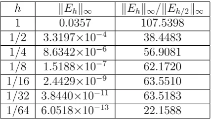
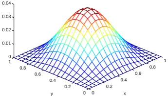
We consider function: u = sin(πx) sin(πy) on [0,1]×[0,1]. Then by using the C2Q5 interpolation introduced in section 2, we can obtain the interpolation function Q5. Figure 17-22 give the plots of the errors on the whole mesh for different h. Table 5 shows grid refinement analysis and the condition numbers of the coefficient matrices, which are obtained

while using the C2Q5 interpolation on [0, h]×[0, h].

order convergent, which satisfies Theorem 4.1. Whenhis smaller than 1/64, round-off error dominates.

Table 5: Grid refinement analysis of C2_Q5 _{interpolation for u= sin(πx) sin(πy)}

h kEhk∞ kEhk∞/kEh/2k∞

1 0.0357 107.5398 1/2 3.3197×10−4 38.4483 1/4 8.6342×10−6 _56.9081

1/8 1.5188×10−7 _62.1720

1/16 2.4429×10−9 _63.5510

0 0.2 0.4 0.6 0.8 1 0 0.2 0.4 0.6 0.8 1 0 0.01 0.02 0.03 0.04 x y

Figure 17: Error ofC2_Q5 _{interpolation}

for u= sin(πx) sin(πy) with h= 1

0 0.5 1 0 0.5 1 0 1 2 3 4

x 10−4

x y

Figure 18: Error ofC2_Q5_{interpolation}

for u= sin(πx) sin(πy) with h= 1/2

0 0.2 0.4 0.6 0.8 1 0 0.2 0.4 0.6 0.8 1 0 0.5 1

x 10−5

x y

Figure 19: Error ofC2Q5 interpolation for u= sin(πx) sin(πy) with h= 1/4

0 0.2 0.4 0.6 0.8 1 0 0.2 0.4 0.6 0.8 1 0 0.5 1 1.5 2

x 10−7

x y

Figure 20: Error ofC2Q5interpolation for u= sin(πx) sin(πy) with h= 1/8

Figure 21: Error ofC2Q5 interpolation for u= sin(πx) sin(πy) with h= 1/16

5

Conclusions and future work

Finite element spaces with certain continuity are more and more commonly used in

math-ematics. The two C2 _{finite elements constructed in section 2 and 3 also can be applied to} some problems. They can be used to solve 2D fourth order partial differential equations,

for example biharmonic equation.

Also, as mentioned in section 1, in [12], the author gives a proof of the convergence order

of the IB method for elliptic interface problems. In the proof, an interpolation function which

is used to interpolate the discrete delta function needs to be constructed. The interpolation

REFERENCES

[1] Finite element method. In Wikipedia. Retrieved June 26, 2012, from http://en.wikipedia.org/wiki/Finite element method.

[2] S. Gilbert and F. George(1973).“ An Analysis of The Finite Element Method. Pren-tice Hall,” ISBN 0-13-032946-0.

[3] R. Coccioli, T. Itoh, G. Pelosi, Peter P. Silvester (1996).“Finite-element methods in microwaves: a selected bibliography.” DOI:10.1109/74.556518.

[4] G. Wolberg and I. Alfy(1999).“Monotonic cubic spline interpolation,”Computer Graph-ics International, 1999. Proceedings, 188-195.

[5] J. C. Fiorot and J. Tabka(1991).“Shape-preserving C2 Cubic Polynomial Interpolat-ing Splines,” Mathematics of Computation vol. 57, no. 195, 291-298.

[6] I. Verlan(2009).“About one algorithem ofC2 interpolation using quartic splines,” Com-puter Science Journel of Moldova, vol.17,no.l(49).

[7] S. Zhang(2010).“On the full C1-QK finite element spaces on rectangles and cuboids,”

Adv. Appl. Math. Mech., 2: 701-721.

[8] J. H. Argyris, I. Fried and D. W. Scharpf(1968).“The TUBA family of plate elements for the matrix displacement method,” Aero.J.Roy.Aero.Soc.,vol. 72, 514-517.

[9] M. J. D. Powell and M. A. Sabin(1977).“Piecewise quadratic approximations on tri-angles,” ACM Trans.Math.Software.,vol. 3-4, 316-325.

[10] F. K. Bogner, R. L. Fox and L. A. Schmit(1965).“The generation of interelement com-patible stiffness and mass matrices by the use of interpolation formulas,”Proceedings of the Conference on Matrix Methods in Structural Mechanics(Wright Patterson A.F.B. Ohio).

[11] C. S. Peskin(1977).“Numerical analysis of blood flow in the heart,”J. Comput. Phys., 25:220-252.