COMPARISON OF UNIFORM HAZARD SPECTRA AND CONDITIONAL
SPECTRA APPROACH IN THE FRAMEWORK OF FRAGILITY CURVE
DEVELOPMENT
Philippe Renault1 and Davide Kurmann2
1
Head of Hazard and Structural Analyses, swissnuclear, Olten, Switzerland ([email protected])
2
Head of Engineering, Nuclear Division, Axpo Power AG, Baden, Switzerland
ABSTRACT
Seismic Probabilistic Safety Assessment (PSA) studies are extensively implemented in risk assessment tools of nuclear power plants and primarily aim to estimate Core-Damage-Frequency (CDF) and Low-Early-Release-Frequency (LERF) based on the expected seismic hazard at a particular site.
In the framework of seismic PSA studies, failure of a structure, system or component is estimated by means of a fragility (probabilistic failure curve), usually defined by means of a median seismic capacity Am, an aleatory variability βR and an epistemic uncertainty βU, based on the Uniform Hazard
Spectrum (UHS) of the underlying seismic hazard study.
This paper wants to illustrate the intrinsic margins buried in the classical approach using UHS compared to when using earthquake scenario spectra (Conditional Spectra - CS) with realistic frequency content. In order to evaluate the benefit of conditional spectra, which on their turn need more computational effort as the traditional UHS based evaluation, a comparison for a (nuclear) structure is performed.
The comparison of the UHS and CS approach in the framework of fragility curve development and the subsequent vulnerability analyses demonstrate the use and potential benefit of the CS. The use of more realistic ground motion input will be discussed in this paper in the context of improving the risk assessment of critical facilities, such as nuclear power plants.
INTRODUCTION
Seismic Probabilistic Safety Assessment (PSA) studies are nowadays extensively implemented in risk assessment tools of nuclear power plants and primarily aim to estimate Core Damage Frequency (CDF) and Low Early Release Frequency (LERF) based on the expected seismic hazard at a particular site. In the framework of seismic PSA studies, failure of a structure, system or component is estimated by means of a fragility (probabilistic failure curve), usually defined by means of a median seismic capacity Am, an aleatory variability βR and an epistemic uncertainty βU (EPRI 2002, 2009).
In order to evaluate the benefit of conditional spectra, which on their turn need more computational effort than the traditional UHS, a comparison of the two approaches for a basic structure is performed. The comparison of the UHS and CS approach in the framework of fragility curve development and vulnerability analyses demonstrates the use and potential benefit of the CS. This comparison is intended as simple illustration and may be extended to a full plant wide assessment if shown successful and economical justifiable. The use of more realistic ground motion input will be discussed in the context of improving the risk assessment of critical facilities. Only if a significant change in terms of out-coming risk (measured e.g. in terms of CDF or LERF) is documented such an approach could find the support from industry. The quantity of “significant” will be subjected to the judgment of the plant risk analyst.
DEVELOPMENT OF HAZARD CONSISTENT UHS, SCENARIO SPECTRA AND TIME HISTORIES
The selection and adjustment of time histories to be used for structural analysis has already been investigated and discussed in the past and is not the focus of this paper. Thus, this section will only repeat the key steps and highlight those relevant for the comparison. Beside numerous journal papers, the interested reader is referred to e.g. NUREG-0800, NUREG/CR-6728, ASCE 4 or NEHRP (2011), Haselton (2009) and Baker et al. (2011).
The UHS are a standard output of the PSHA and described in terms of mean curve and requested fractiles (e.g. 0.05, 0.16, 0.50, 0.84, 0.95, or much more). The UHS are usually provided for all requested annual probabilities of exceedance (e.g. 10-2 to 10-7) and a common assumption made for the subsequent analysis is that the UHS at an annual probability of exceedance of 10-4 is representative in shape and characteristics to be scaled to the other relevant annual probability levels. The smooth UHS on the bedrock level usually matches this simplification. Together with the deaggregation results from the PSHA the dominant magnitudes and distances are defined and characterize the relevant scenarios to be modeled as input to dynamic analyses.
In the classical approach the analyst selects a suite of preferably recorded seed time histories from the available strong motion databases which fit the basic magnitude and distance requirements defined through the deaggregation information. Furthermore, duration, site conditions, appropriate spectral content, focal mechanism and depth are sometimes used to constrain the selected time histories.
The set of selected time histories (e.g. 30 three-component time histories) is then usually fitted to match the mean UHS and the time histories are scaled in amplitude to the corresponding spectral amplitude of the UHS for the other annual probabilities of exceedance. The selected time histories can be modified to be compatible with the earthquake spectrum either by scaling (multiplying by a constant) or by changing the frequency content while maintaining the non-stationary character of the initial ground motion (spectral matching). The constraining reference frequency can e.g. be PGA or a structural relevant frequency (first eigen-frequency) and needs to be consistent with the frequency for which the fragility curves are developed.
The geometrical mean of the two selected horizontal components of the response spectra of the seed time histories should to be compatible with the UHS (which represents the geom. mean. component resulting from the hazard analysis). Variability of the two horizontal components about the geom. mean should be included and each horizontal time history component should represent a realistic spectrum and not necessarily match closely the UHS at each frequency. Usually, 30 three component records are selected. The average of the 30 geometrical means of the two horizontal components or the ensemble of the 30 vertical components is then used to check the matching criteria with respect to the horizontal and vertical UHS, respectively. Often used matching criteria are e.g. defined in NUREG-0800 or NUREG/CR-6728.
The so called Conditional Mean Spectrum (CMS) and Conditional Spectra (CS) approach are a more formal way of defining hazard consistent time histories. The median of the conditional spectra is given by the Conditional Mean Spectra (Baker & Cornell, 2006a,b). The development of the median scenario spectrum is based on the computation of the epsilon value required to scale the median spectrum to match exactly the UHS for the given spectral frequency. The mean epsilons at the other spectral frequencies, conditioned on the epsilon at the selected frequency, are then used to develop the conditional mean spectrum. The variability about the median spectrum is captured by taking 30 realizations (named conditional spectra, CS) of the epsilon variability about the CMS, accounting for the correlation of the epsilons between different frequencies. This process is repeated for each selected hazard level and for each magnitude-distance bin. A rate of occurrence is determined for each scenario such that the combined rates from the scenarios approximate the hazard. This results in a large number of scenario spectra, but they have the advantage that they reproduce the full hazard at each spectral frequency more accurately than a simplified approach, for example as proposed e.g. in Abrahamson and Yunatci (2010). At each spectral frequency, the UHS includes the effect of peak-to-trough variability through the standard deviation of the ground motion model. The peak-to-trough variability about the scenario spectra is estimated by means of the correlations of the ground motion variability between different spectral frequencies, as shown by Abrahamson and Al Atik (2010). This range of peak-to-trough variability can be used for guidance when selecting time histories with the appropriate peak-to-trough variability.
Lin et al. (2013) have described the framework on how to accommodate multiple ground motion prediction equations (GMPE) in the CS approach and compared different simplification methods. The following four methods have been discussed there:
Method 1: Approximate CS using mean M/R and a single GMPE
Method 2: Approximate CS using mean M/R and GMPEs with logic-tree weights
Method 3: Approximate CS using GMPE-specific mean M/R and GMPEs with deaggregation weights
Method 4: “Exact” CS using multiple causal earthquake M/R and GMPEs with deaggregation weights
In real practice the use of multiple GMPEs and experts, as for example in a SSHAC (1997) process, sets clear practical limits to the approach illustrated by Lin et al. (2013). One of the obvious issues being the consideration of multiple experts using the same GMPEs, but with different weights and maybe adjustments. Furthermore, the evaluation of a Nuclear Power Plant (NPP) implies that there is not a single reference frequency, as multiple structures and components are to be assessed and thus, the conditioning frequency should ideally be a range and not a single value. In the framework of the PEGASOS Refinement Project (Renault et al., 2010, Renault, 2011, 2012, Renault and Abrahamson, 2013) an approximate, but still fully consistent approach has been developed and is very similar to the method 2 and 3 of Lin et al. (2013). The “PRP approach” is described in the following.
The approach approximates the CS using mean M/R and GMPEs combined according to their contribution. The idea is to combine individual GMPEs of each expert according to their contribution (deaggregation) per annual probability of exceedance (APE), but using one mean M and R for all GMPEs per APE. For this, one set of mean source characteristics for all GMPEs is used. Furthermore, a mean hypocentral depth for all GMPEs per APE is defined and used for the V/H ratios, representing an extension compared to Lin et al. (2013)
Step 1: Definition of the conditioning frequency f0/range for the site
In general the relevant frequency range for the assessment is between 2.5 and 25 Hz (depending on the structure to analyze). The center of this range is represented by its geometrical mean, which is approx. 8 Hz and is then defined as the conditioning frequency f0. For consistency with the fragility
analysis it is recommended to use the spectral frequency which is used for the NPP fragility evaluation as the reference frequency f0, as everything is conditioned on this frequency.
Step 2: Evaluation of individual GMPE contributions
The hazard analysis needs to generate a table for the specified conditioning period which contains the individual GMPE contributions to the mean hazard for each annual probability of exceedance for the site based on the site deaggregation for f0. (In the following it is implied that the analysis is developed for
the conditioning frequency f0 and thus, f0 is dropped as index.)
Table 1 Schematic overview table for evaluating the GMPE contributions to the total hazard
Contributions per Annual Probability of Exceedance
1E-2 1E-3 1E-4 1E-5 1E-6 1E-7 1E-8
SA_MeanHaz(APE) SAvalue …
GMPE_1 Contrib.
GMPE_2 …
…
Where GMPE_i represents the mean hazard for the GMPE number i based on each expert and his specific corrections (e.g. host-to-target correction for shear wave velocity and Kappa). This can result in multiple versions of a GMPE, but where each depends on a different underlying distribution of correction factors. The GMPE name and expert name corresponding to GMPE_i should be stored in order to be able to identify them clearly for the subsequent computation. The mean hazard refers to the total mean over all experts.
𝐶𝑜𝑛𝑡𝑟𝑖𝑏(𝐺𝑀𝑃𝐸_𝑖,𝐴𝑃𝐸) = 𝐴𝑃𝐸𝐴𝑃𝐸(𝐺𝑀𝑃𝐸(𝑚𝑒𝑎𝑛_𝑖│ℎ𝑎𝑧𝑎𝑟𝑑𝑆𝐴(𝐴𝑃𝐸)))
Step 3: Definition of magnitude and distance pairs and associated source parameters
Through deaggregation for the different annual probabilities of exceedance, the contribution for different magnitude and distance bins for all combinations of logic tree branches for a single specified spectral frequency are determined. If the deaggregation is only available for a subset of APE, it is convenient to interpolate the missing ones based on a grid approach. Nevertheless, the change of mean M and R with smaller APE level should be checked in order to verify the accuracy of an interpolation.
Table 2 Template table summarizing the mean magnitude (M), mean distance (R), and depth (H)
Mean Mag. and Dist. per Annual Probability of Exceedance
1E-2 1E-3 1E-4 1E-5 1E-6 1E-7 1E-8
Mean M(f0) …
Mean R(f0)
The source parameters are defined based on the host sources and main contributors, respectively:
• Style of faulting (e.g. strike slip)
• Dip angle
Step 4: Evaluate horizontal response spectra and V/H ratio for all parameters and GMPEs
Various source parameters with associated weights have been defined and used in the logic tree approach and used in the evaluation for the V/H ratios. Strictly speaking the same could be done also for the response spectra evaluation for each GMPE. For the sake of efficiency and as the representative median response spectra is not used to develop directly time histories, the project has decided to simplify the evaluation by only using the dominant and representative set of source parameters. Thus, the response spectra and V/H ratios are only evaluated for the style of faulting and dip angle defined in step 3 (instead of using all style of faulting and dip angels, for which the resulting spectra would need to be combined according to the source parameter weights). The response spectra and V/H ratios need to be evaluated at the same frequencies in order to be compatible.
Note: Alternatively to the V/H ratios for each APE level, a vertical response spectra can also be used directly.
Step 5: Evaluation of the representative median acceleration spectrum
The representative median response spectrum (interpreted as geometrical mean of the two horizontal components) is obtained by summing all individual spectral accelerations of the GMPEs multiplied with their contribution of step 2.
ln (𝑀𝑒𝑑𝑖𝑎𝑛𝑆𝐴(𝑓,𝐴𝑃𝐸)) = ∑𝐺𝑀𝑃𝐸𝑛 𝑖=1[ ln (𝑆𝐴(𝐺𝑀𝑃𝐸𝑖,𝑓)) ∙ 𝐶𝑜𝑛𝑡𝑟𝑖𝑏 (𝐺𝑀𝑃𝐸_𝑖,𝐴𝑃𝐸)] (1)
For the vertical component the representative acceleration response spectrum is derived in our case with V/H ratios as such that
𝑉𝑒𝑟𝑡𝑖𝑐𝑎𝑙𝑀𝑒𝑑𝑖𝑎𝑛𝑆𝐴(𝑓,𝐴𝑃𝐸) =𝐻𝑜𝑟𝑖𝑧𝑜𝑛𝑡𝑎𝑙𝑀𝑒𝑑𝑖𝑎𝑛𝑆𝐴(𝑓,𝐴𝑃𝐸) ×𝑚𝑒𝑑𝑖𝑎𝑛𝑉𝐻(𝑓,𝐴𝑃𝐸). (2)
Step 6: Evaluation of aleatory variability
After having calculated the response spectrum to be used for the analysis, also an aleatory variability about the spectrum needs to be defined. Within the project this aleatory variability has been computed based on the various expert models and weights. The values have to be available in dependency of frequency for the required APE levels and need to be interpolated if necessary. As in our case the V/H ratios have been used to come up with a vertical spectrum, only an additional aleatory variability term about the vertical was added. As the horizontal already contains aleatory variability, it is necessary to only add something in case it is present and to avoid double-counting of uncertainties.
Step 7: Computation of Scenario Spectra
The scenario spectra for the horizontal and vertical component are computed in the last step by using all products of the previous steps and the horizontal and vertical UHS per APE. Those are:
• Conditioning frequency (which is assumed to be the same for horizontal and vertical)
• Median horizontal response spectra and V/H ratios per APE (step 5)
The output of the procedure is a list of scenario spectra, rates, scaling factors and some meta data. Furthermore, comparison plots of the computed horizontal & vertical hazard curves, comparisons of the target and computed horizontal & vertical UHS curves, horizontal and vertical calculated CMS curves, and a list of all the time histories defined in a flatfile and based on the identified unique scenario spectra. Conditional Spectra are a means to the end result (time histories), not the result itself.
The advantage of this procedure is that it allows considering multiple expert contributions, even if using the same basic GMPEs, and preserves computational efficiency, as it is only necessary to evaluate one resulting representative (median) response spectrum. According to Lin et al. (2013) this proposed approach is equivalent to the «exact» solution if the M and R deaggregation is stable (unimodal) over APE and the used GMPEs all have similar spectral shape and epsilons.
DYNAMIC ANALYSIS OF A NUCLEAR STRUCTURE AND RESULTS
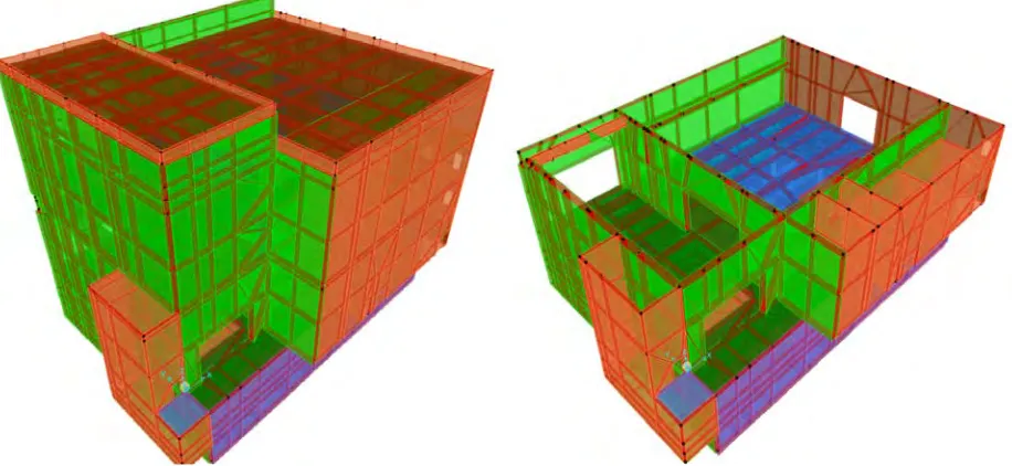
In order to evaluate the benefits of the CS versus UHS method, linear modal history analyses have been carried out with SAP2000. For this purpose, a 3D finite element (FE) structural model of an existing, safety and radiological relevant building on a Swiss NPP site has been used. The structure consists of a four-storey reinforced concrete shear wall building with a total height of H = 29.50 m above foundation plate (elevation -7.50 m). Plan metric building dimensions are L x W = 33.80 m x 21.40 m. An overhanging section with dimensions L x W = 22.00 m x 5.00 m extends on the east facade and is structurally monolithic connected with the main building (Figure 1). Primary bearing capacity is carried by external and internal shear walls in longitudinal (NS) respectively in transverse direction (EW).
Figure 1. South-East perspective view of the complete 3D FE structural model (left), respectively of ground floor level (right) as implemented in SAP2000.
Modal analysis has been carried out taking into consideration 20 modes. Modal results for best-estimate soil properties shows a range of horizontal, fundamental frequencies between f = 3.7 – 4.1 Hz; typical for nuclear structures (see Table 3).
Table 3: Summary of modal analysis results for the 3D FE structural model. X- (NS) and Y-direction (EW) lie in horizontal plane, Z-direction is vertical.
Mode Frequency Damping Ratio Mass Ratio MX Mass Ratio MY Mass Ratio MZ
[-] [Hz] [-] [-] [-] [-]
1 3.68 0.07 0.001 0.70 -
2 4.12 0.07 0.735 0.002 -
4 8.09 0.07 0.002 0.002 0.895
5 9.90 0.07 0.183 0.006 0.025
6 10.1 0.07 - 0.214 -
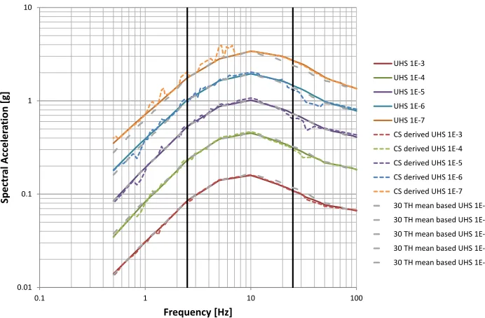
As defined in the second chapter, two seeds of three-component time histories based on the UHS and CS, have been used in order to compare the benefits of the CS method in terms of base reactions and in-structure-response-spectra (ISRS) compared with the UHS based approach. As starting point, the geometrical mean of the thirty seeds of time histories based on the 10-4/yr UHS scaled to other levels, and the geometrical mean of the seeds of time histories based on the CS approach for a range of annual probabilities of exceedance are compared in figure 2.
Figure 2. Comparison of horizontal UHS (solid colored lines), represented as result of PSHA by the geom. mean of the two horizontal components, and geom. mean spectra of the thirty time histories based
on the UHS approach (grey dashed lines), and of the scenario time histories based on the CS approach (dashed colored lines) for APE of 10-3/yr to 10-7/yr. The two vertical lines at 2.5 and 25 Hz represent the range of the selected required strict matching of the scenario based CS to the target UHS. Below 1 Hz the
looser criteria are obvious, but outside the relevant frequency range of interest for the analyzed structure. 0.01
0.1 1 10
0.1 1 10 100
Sp
ect
ra
l Acce
le
ra
tion
[g
]
Frequency [Hz]
Linear dynamic analyses on the 3D structural models yields for this example to conservative results for the UHS compared with the CS approach. Even if strictly speaking the comparison of individual results at a single APE is not meaningful, as only the overall probability of failure and resulting risk can be compared, some ISRS based on analyses for 10-4/yr are illustrate here for discussion. Nevertheless, at the conditioning frequency theses individual extracted results can be compared directly.
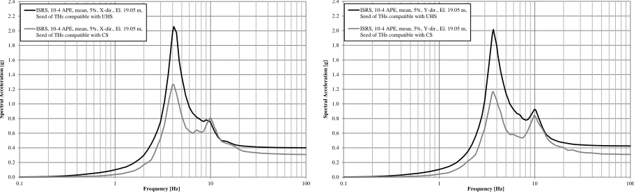
The maximal base shear forces (mean values) based on CS time histories are in this case 15-17% lower compared with the UHS method. Maximal overturning moments (mean values) based on CS are even 26-29% lower compared with UHS method. ISRS at the roof level for both horizontal directions yield to considerable lower results for CS compared with UHS. In the low frequency range f < 7 Hz the spectral acceleration has been reduced by 40%, while in the high frequency range f > 20 Hz spectral accelerations decreases by 20% (Figure 3). As already mentioned, the decrease beside the conditioning frequency is only indicative, but show the average tendency.
Figure 2. Illustrative example of ISRS, APE 10-4/yr, mean, 5% damping ratio, roof level for the X- (NS-) (left), respectively Y- (EW) direction (right) resulting from UHS-method (black) and CS-method (grey)
CONCLUSION
Objective of the earthquake scenario spectra based approach is to find a set of scaled time histories and rates of occurrence that have realistic spectral variation and replicate the hazard over a broad range of spectral frequency and hazard levels. The procedure uses conditional spectra to select candidate time histories. The benefit is that it avoids the conservatism of the UHS motions, which assume that high amplitudes occur at all frequencies and orientations in a single ground motion. The cost is that a greater number of ground motions (analyses) will be required compared to the classical UHS based approach. Furthermore, it needs to be understood that each time history will be treated as an initiating event in system risk calculations. It can be anticipated to obtain 50-80 unique time histories and ~600 total time histories after scaling to multiple amplitudes over the range from APE 10-3 to 10-7/yr. This differs from the treatment of UHS based time histories (usually 30 for the central APE and scaled to the other levels). As long as the structural analysis is performed in the linear domain the CS based approach also allows to make use of the smaller amount of unique time histories and scale the results to the corresponding levels of the total amount of necessary time histories (~600).
For the example evaluated in the framework of this paper, the additional computational effort for the scenario spectra approach lead to a meaningful reduction of seismic forces (i.e. ISRS) and therefore lead to higher fragilities compared to the UHS method. Results of the presented example indicate that benefits of scenario time histories based on an approach consistent with the seismic hazard assessment may be different depending on the dynamic properties of an analyzed structure, system or component (frequency dependence) but tend to be lower.
0.0 0.2 0.4 0.6 0.8 1.0 1.2 1.4 1.6 1.8 2.0 2.2 2.4
0.1 1 10 100
S p ect ra l A ccel era ti o n [ g ] Frequency [Hz]
ISRS, 10-4 APE, mean, 5%, X-dir., El. 19.05 m, Seed of THs compatible with UHS
ISRS, 10-4 APE, mean, 5%, X-dir., El. 19.05 m, Seed of THs compatible with CS
0.0 0.2 0.4 0.6 0.8 1.0 1.2 1.4 1.6 1.8 2.0 2.2 2.4
0.1 1 10 100
S p ect ra l A ccel era ti o n [ g ] Frequency [Hz]
ISRS, 10-4 APE, mean, 5%, Y-dir., El. 19.05 m, Seed of THs compatible with UHS
As a next step a comparison of developed fragility curves based on both approaches will be performed in order to investigate the effect of the scenario based approach. Furthermore, a more systematic assessment, including detailed soil-structure-interaction (SSI) analyses, of varying geometry and structural properties will be performed in order to further demonstrate the benefit of this consistent approach.
REFERENCES
Abrahamson, N.A. and Al Atik, L. (2010). “Scenario Spectra for Design Ground Motions and Risk Calculations”, 9th US National & 10th Canadian Conference on Earthquake Engineering: Reaching Beyond Borders, July 25-29, Toronto, Canada.
Abrahamson, N.A. and Yunatci, A.A., (2010). “Ground Motion Occurrence Rates for Scenario Spectra”, 5th Int. Conf. on Recent Advances in Geotechnical Earthquake Engineering and Soil Dynamics, May 24-29, San Diego, California.
Baker J.W. and Cornell C.A. (2005). “A Vector-Valued Ground Motion Intensity Measure Consisting of Spectral Acceleration and Epsilon”, Earthquake Engineering & Structural Dynamics, 34 (10), 1193-1217.
Baker, J.W. and Cornell, C.A. (2006). “Spectral shape, epsilon and record selection”, Earthquake Engineering and Structural Dynamics, 35, 1077–1095.
Baker, J.W. and Cornell, C.A. (2006), “Vector-Valued Ground Motion Intensity Measures for Probabilistic Seismic Demand Analysis”, PEER Report No. 2006/08.
Baker, J. W.; Lin, T.; Shahi, S. K. & Jayaram, N. (2011). “New Ground Motion Selection Procedures and Selected Motions for the PEER Transportation Research Program”, report PEER 2011/03.
EPRI (2002), Seismic Fragility Application Guide, Report 1002988.
EPRI (2009), Seismic Fragility Applications Guide Update, Report 1019200.
Haselton, C. B. (2009). “Evaluation of Ground Motion Selection and Modification Methods: Predicting Median Interstory Drift Response of Buildings”, PEER Ground Motion Selection and Modification Working Group, report PEER 2009/01.
Lin, T.; Harmsen, S.; Baker, J. & Luco, N. (2013). “Conditional Spectrum Computation Incorporating Multiple Causal Earthquakes and Ground Motion Prediction Models”, Bulletin of Seismological Society of America, 103(2a).
NEHRP Consultants Joint Venture (2011) “Selecting and Scaling Earthquake Ground Motions for Performing Response- History Analyses”, report NIST GCR 11-917-15.
NRC (2007). “Standard Review Plan for the Review of Safety Analysis Reports for Nuclear Power Plants”, NUREG-0800.
NRC (2001). “Technical Basis for Revision of Regulatory Guidance on Design Ground Motions: Hazard- and Risk-consistent Ground Motion Spectra Guidelines”, NUREG/CR-6728.
Renault, P.; Heuberger, S. and N.A. Abrahamson (2010). “PEGASOS Refinement Project: An improved PSHA for Swiss nuclear power plants”. In proceedings of 14th European Conference on Earthquake Engineering, 30. August to 3. September 2010, Ohrid, Republic of Macedonia.
Renault, P. (2011). “PEGASOS Refinement Project: New findings and Challenges from a PSHA for Swiss Nuclear Power Plants”, Paper 561, SMiRT 21, November 6-11, 2011, New Delhi, India.
Renault, P. (2012). “Approach and Challenges for the Seismic Hazard Assessment of Nuclear Power Plants – The Swiss Experience”, Bollettino di Geofisica Teorica ed Applicata - Special issue for GNGTS.
Renault, P. and N.A. Abrahamson (2013). “Lessons learned from the seismic hazard assessment of NPPs in Switzerland”, SMiRT 22, Special Session on New Developments for Ground Motion Prediction for Stable Continental Regions and NGA-East, August 18-23, San Francisco, California, USA.