Component Selection and Smoothing in Smoothing Spline
Analysis of Variance Models
By Yi Lin AND Hao Helen Zhang
University of Wisconsin - Madison and North Carolina State University
Abstract
We propose a new method for model selection and model fitting in nonparametric regression models, in the framework of smoothing spline ANOVA. The “COSSO” is a method of regularization with the penalty functional being the sum of component norms, instead of the squared norm employed in the traditional smoothing spline method. The COSSO provides a unified framework for several recent proposals for model selection in linear models and smoothing spline ANOVA models. Theoretical properties, such as the existence and the rate of convergence of the COSSO estimator, are studied. In the special case of a tensor product design with periodic functions, a detailed analysis reveals that the COSSO applies a novel soft thresholding type operation to the function components and selects the correct model structure with probability tending to one. We give an equivalent formulation of the COSSO estimator which leads naturally to an iterative algorithm. We compare the COSSO with the MARS, a popular method that builds functional ANOVA models, in simulations and real examples. The COSSO gives very competitive performances in these studies.
Key words and phrases: LASSO, method of regularization, model selection, nonnegative garrote, nonparametric regression, variable selection.
1
Introduction
Consider the regression problem yi = f(xi) +ǫi, i = 1, ..., n, where f is the unknown
regression function to be estimated, xi = (x(1)i , ..., x
(d)
i )’s are d dimensional vectors of
co-variates, and the ǫ’s are independent noises with mean 0 and variance σ2. Usually the
estimator is judged in terms of prediction accuracy and interpretability.
In linear regression models it is assumed that f(x) = β0 +Pdj=1βjx(j). Traditional
approaches to variable selection include the best subset selection and the forward/backward stepwise selection. As pointed out by Breiman (1995), these methods suffer from instability and relative lack of accuracy. Several new and effective methods for variable selection in linear models have been proposed in recent years [Breiman (1995); Tibshirani (1996); Frank and Friedman (1993); Fan and Li (2001)]. Two methods, the nonnegative garrote by Breiman (1995) and the LASSO by Tibshirani (1996), are closely related to the method in our paper, and are reviewed in the following.
Assume that the x(ij)are standardized so thatP
ix
(j)
i /n= 0 and
P
i{x
(j)
i }2/n= 1. Let
ˆ
is ( ˆβo
0, r1βˆ1o, ..., rdβˆdo), where (r1, ..., rd) is the solution to
min
r1,...,rd
n
X
i=1
{yi−βˆ0o−
d
X
j=1
rjβˆojx(ij)}2, subject to rj ≥0, j= 1, ..., d, and d
X
j=1 rj ≤t.
Here t ≥ 0 is a tuning parameter. The nonnegative garrote selects subset and shrinks the estimate at the same time. Breiman (1995) showed that the nonnegative garrote has consistently lower prediction error than subset selection with extensive simulation studies. The Least Absolute Shrinkage and Selection Operator (LASSO) estimate ˆβ = ( ˆβ0, ...,βˆd)
is the minimizer of
1
n
n
X
i=1
{yi−β0−
d
X
j=1
βjx(ij)}2 subject to d
X
j=1
|βj| ≤t,
or equivalently, the minimizer of
1
n
n
X
i=1
{yi−β0−
d
X
j=1
βjx(ij)}2+λ d
X
j=1 |βj|,
wheretorλare tuning parameters. The LASSO is a penalized least squares method with the
L1 penalty on the coefficients. Tibshirani (1996) proposed and studied the LASSO. Bakin
(1999) contained some useful developments. Knight and Fu (2000) studied the asymptotic properties of the LASSO.
We consider model selection in a more general nonparametric setting, within the smooth-ing spline analysis of variance (SS-ANOVA) framework [Wahba (1990); Wahba, Wang, Gu, Klein and Klein (1995); Gu (2002)]. In the SS-ANOVA we write
f(x) =b+
d
X
j=1
fj(x(j)) +
X
j<k
fjk(x(j), x(k)) +· · ·, (1)
where b is a constant, fj’s are the main effects, fjk’s are the two way interactions, and
manner. Gunn and Kandola (2002) proposed a sparse kernel approach in a closely related framework. Zhang, Wahba, Lin, Voelker, Ferris, Klein and Klein (2002) gave a possible generalization of the LASSO to the SS-ANOVA for exponential families. They expanded each nonparametric component function as a linear combination of a large number of basis functions, and applied L1 penalty to the coefficients of all the basis functions. The L1
penalty gives a solution that is sparse in the coefficients. However, a separate model selection procedure has to be applied after model fitting, since sparsity in coefficients helps but does not guarantee the sparsity in SS-ANOVA components.
In this paper we consider a different approach for model selection and model fitting in the SS-ANOVA. This is a method of regularization with the penalty functional being the sum of component norms. We show that the approach provides a unified framework for several recent proposals for model selection in linear models and SS-ANOVA models. The new method reduces to the LASSO in linear models, and thus gives an alternative interpretation of the penalty term in the LASSO to being theL1 norm of the coefficients:
it is the sum of component norms. Our method will be referred to as the COmponent Selection and Smoothing Operator (COSSO). The general methodology is introduced in Section 2, where we also prove the existence of the COSSO estimate and give some rate of convergence results. In Section 3 we obtain an alternative formulation of the COSSO that is more suitable for computation. In Section 4, we consider the special case of a tensor product design with periodic functions. A detailed analysis in this special case sheds light on the mechanism of the COSSO in terms of component selection in the SS-ANOVA. In particular, we show in this case, that the COSSO applies a novel soft thresholding type operation to the function components and selects the correct model structure with probability tending to one. In Section 5, we present a COSSO algorithm that is based on iterating between the smoothing spline method and the nonnegative garrote. In Section 6, we consider the choice of the tuning parameter. Simulations are given in Section 7, where we compare the COSSO with the MARS developed by Friedman (1991), a popular algorithm that builds functional ANOVA models. Some real examples are given in Section 8, and Section 9 contains a discussion. The proofs are given in the Appendices.
2
The COSSO in smoothing spline ANOVA
2.1 The smoothing spline ANOVA
Hj ={1} ⊕H¯j. Then the tensor product space of theHj’s is
⊗dj=1Hj ={1} ⊕
d
X
j=1
¯
Hj⊕X
j<k
[ ¯Hj⊗H¯k]⊕ · · ·. (2)
Each functional component in the SS-ANOVA decomposition (1) lies in a subspace in the orthogonal decomposition (2) of⊗dj=1Hj. Typically only low order interactions are consid-ered in the SS-ANOVA model for interpretability and visualization. The popular additive model is a special case in which f(x(1), ..., x(d)) = b+Pd
j=1fj(x(j)), with fj ∈ H¯j. In
this case the selection of functional components is equivalent to variable selection. In more complex SS-ANOVA models model selection amounts to the selection of main effects and interaction terms in the SS-ANOVA decomposition. The interaction terms reside in the tensor product spaces of univariate function spaces. The reproducing kernel of a tensor product space is simply the product of the reproducing kernels of the individual spaces. This greatly facilitates the use of smoothing spline type method in such models.
A common example of the function space Hj of univariate functions, which is also used in this paper, is the second order Sobolev Hilbert space: S = {g : g, g′ are absolutely
continuous,g′′
∈ L2[0,1]}. When endowed with the norm
kgk2 ={
Z 1
0
g(t) dt}2+{
Z 1
0
g′(t) dt}2+
Z 1
0 {
g′′(t)}2 dt,
S can be decomposed as S = {1} ⊕S¯, where ¯S is a RKHS with the reproducing kernel ¯
K(s, t) =k1(s)k1(t) +k2(s)k2(t)−k4(|s−t|), withk1(t) =t−1/2,k2(t) ={k12(t)−1/12}/2,
and k4(t) ={k41(t)−k12(t)/2 + 7/240}/24. See Wahba (1990), Gu (2002).
2.2 The COSSO
In general, the function space in SS-ANOVA can be written as
F ={1} ⊕ F1, with F1 =
p
M
α=1
Fα, (3)
to select parametric and nonparametric components of the variables.
Denote the norm in the RKHS F by k · k. A traditional smoothing spline type method findsf ∈ F to minimize
1
n
n
X
i=1
{yi−f(xi)}2+λ p
X
α=1 θ−1
α kPαfk2, (4)
where Pαf is the orthogonal projection of f onto Fα and θ
α ≥ 0. If θα = 0, then the
minimizer is taken to satisfy kPαfk2 = 0. We use the convention 0/0 = 0 throughout this paper. The smoothing parameterλ is confounded with the θ’s, but is usually included in the setup for computational purpose.
We propose the COSSO procedure that finds f ∈ F to minimize
1
n
n
X
i=1
{yi−f(xi)}2+τn2J(f), with J(f) = p
X
α=1
kPαfk, (5)
where τn is a smoothing parameter. We sometimes suppress the dependence of τ on n in
our notation. The penalty term J(f) in the COSSO is a sum of RKHS norms, instead of the squared RKHS norm penalty employed in the smoothing spline. The penalty J(f) is not a norm in F. However, it is a pseudo-norm in the sense: for any f, g in F, J(f) ≥ 0, J(cf) =|c|J(f), J(f+g)≤J(f) +J(g); for any nonconstantf inF, J(f)>0. And we have that
p
X
α=1
kPαfk2 ≤J2(f)≤p
p
X
α=1
kPαfk2. (6)
Another difference between the COSSO and the common smoothing spline method is that there is only one smoothing parameterτ in the COSSO procedure (5), while in the common smoothing spline approach (4) there are multiple smoothing parameters.
The LASSO in linear models can be seen as a special case of the COSSO. For the input spaceX = [0,1]d, consider the linear function spaceF ={1}⊕{x(1)−1/2}⊕...⊕{x(d)−1/2}, with the usual L2 inner product on F: (f, g) =
R
Xf g. The penalty term in the COSSO
becomes J(f) = (12)−1/2Pd
j=1|βj|for f(x) = β0+ Pd
j=1βjx(j). This is equivalent to the L1 norm on the linear coefficients, leading to the LASSO estimator. Notice, however, we
interpret the penalty as the sum of the norms of the function components, rather than the
L1 norm of the coefficients.
2.3 Existence of solution to the COSSO
Theorem 1 Let F be a RKHS of functions over an input space X. Assume that F can be
decomposed as in (3). Then there exists a minimizer of (5) in F.
It is of interest to characterize the conditions under which the solution to (5) is unique. It seems the uniqueness should follow under mild conditions on the design matrix of the input variables. We do not pursue this question here, and the development in this paper does not depend on the uniqueness of the COSSO estimate.
2.4 Asymptotic properties of the COSSO
In this section we assume a fixed design. Define y = (y1, ..., yn)T. With a little abuse of
notations, let f stand for both the regression function and its functional values at data points, i.e., f = (f(x1), ..., f(xn))T. Define the norm k · kn and inner product h·,·in in Rn
as
kfk2n= 1
n
n
X
i=1
f2(xi), hf, gin=
1
n
n
X
i=1
f(xi)g(xi);
then ky−fk2n = 1/nPn
i=1{yi −f(xi)}2. The following theorem shows that the COSSO
estimator in the additive model has a rate of convergencen−2/5 if the tuning parameter is
chosen appropriately.
Theorem 2 Consider the regression model yi = f0(xi) +ǫi, i = 1, ..., n, where xi’s are
given covariates in [0,1]d, and ǫ
i’s are independent N(0, σ2) noises. Assume f0 lies in
F = {1} ⊕ F1, F1 =Ldj=1S¯j, with Sj ={1} ⊕S¯j being the second order Sobolev space.
Consider the COSSO estimate fˆas defined in (5). Then (i) if f0 is not a constant, and
τ−1
n =Op(n2/5)J3/10(f0), we havekfˆ−f0kn=Op(τn)J1/2(f0); (ii) if f0 is a constant, we
have kfˆ−f0kn=Op(max{(nτn)−2/3, n−1/2}).
Results for more general ANOVA models can be obtained in a similar way. For example, since the tensor product space of two second order Sobolev spaces of univariate functions is a subspace of the second order Sobolev space of bivariate functions, we can obtain that the COSSO estimator in the two way interaction model has a rate of convergence that is at least as fast as n−1/3. This rate is not the optimal rate for SS-ANOVA models. See Lin (2000).
However, to prove better rates for the COSSO estimator, involved entropy calculations for tensor product spaces will be required.
3
An equivalent formulation
Lemma 1 Let fˆ= ˆb+Pp
α=1fˆα be a minimizer of (5) in (3), with fˆα ∈ Fα. Then fˆα ∈
span{Rα(xi,·), i= 1, ..., n}, whereRα(·,·) is the reproducing kernel of the space Fα.
However, it is possible to give an equivalent form of (5) that is easier to compute. Consider the problem of findingθ= (θ1, ..., θp)T and f ∈ F to minimize
1
n
n
X
i=1
{yi−f(xi)}2+λ0
p
X
α=1
θ−α1kPαfk2+λ
p
X
α=1
θα, subject to θα ≥0, α= 1, ..., p, (7)
where λ0 is a constant that can be fixed at any positive value, and λ(n) is a smoothing
parameter. We will fix λ0 at some value for computational considerations.
Lemma 2 Set λ = τ4/(4λ
0). (i) If fˆ minimizes (5), set θˆα = λ01/2λ−1/2kPαfˆk, then the
pair (ˆθ,fˆ) minimizes (7). (ii) On the other hand, if a pair (ˆθ,fˆ) minimizes (7), then fˆ
minimizes (5).
The form of (7) is very similar to the common smoothing spline (4) with multiple smoothing parameters, except that there is an additional penalty on the θ’s. Notice that there is only one smoothing parameter λ in (7). The θ’s are part of the estimate, rather than free smoothing parameters. The additional penalty on θ’s in (7) makes it possible to have someθ’s be zeros, giving rise to zero function components in the COSSO estimate. In contrast, the common smoothing spline has two sets of smoothing parametersλandθ’s that are confounded. The common way to search for smoothing parameters iterates betweenλ
and logθ’s, making it difficult to have zero components in the solution.
4
A special case with the tensor product design
In this section we consider the special case of a tensor product design with a SS-ANOVA model built from the second order Sobolev spaces of periodic functions (functions on the circle). The function space of the SS-ANOVA is then (2) withH’s being the second order Sobolev spaces of periodic functions. This is a subspace ofSconsisting of periodic functions, and can be written asT ={1} ⊕T¯, where
¯
T ={f :f(t) =
∞
X
ν=1 aν
√
2 cos 2πνt+
∞
X
ν=1 bν
√
2 sin 2πνt, with
∞
X
ν=1
(a2ν+b2ν)(2πν)4<∞}.
The reproducing kernel of ¯T is ¯K(s, t) = −k4(|s− t|), and the norm in ¯T is kgk2 = R1
0{g
′′
subspace ofT is Tm ={1} ⊕T¯m, with
¯
Tm ={f :f(t) = m/2−1
X
ν=1 aν
√
2 cos 2πνt+
m/2−1 X
ν=1 bν
√
2 sin 2πνt+am/2cosπmt}.
Wahba (1990) used this subspace approximation to give a very instructive investigation of the filtering properties of the smoothing spline.
We assume that the data points follow a tensor product design. That is, the design points are
{(xi1,1, xi2,2, ..., xid,d) :ik= 1, ..., nk, k= 1, ..., d},
where xj,k = j/nk, j = 1, ..., nk, k = 1, ..., d. Therefore the total sample size is n =
n1 · · ·nd. We assume the ǫ’s in the regression model are independent with distribution
N(0, σ2). We give a detailed treatment that sheds light on the mechanism of the COSSO for model selection, and show that under mild conditions, the COSSO selects the correct model structure with probability tending to one.
Without loss of generality, we fix λ0 = 1 in the COSSO (7) and focus on the case of d= 2,n1 =n2=m, and the SS-ANOVA model contains three componentsf1,f2, andf12.
In this situation any f ∈ F can be written as f(s, t) =b+f1(s) +f2(t) +f12(s, t), with
f1 ∈T¯1,f2 ∈T¯2, and f12∈T¯1⊗T¯2, and (7) becomes
1 n m X k=1 m X ℓ=1
{ykl−f(xk,1, xℓ,2)}2+θ−11 Z 1
0
∂2f1(s) ∂s2
2
ds+θ2−1 Z 1
0
∂2f2(t) ∂t2
2 dt
+ θ−121 Z 1
0 Z 1
0
∂4f 12(s, t) ∂s2t2
2
dsdt+λ(θ1+θ2+θ12), with θ1 ≥0, θ2≥0, θ12≥0.
We start with an argument for an approximate subspace of F, and then move on to the space F. Assume m is even, and define Fm =Tm1 ⊗Tm2 = {1} ⊕T¯m1 ⊕T¯m2 ⊕( ¯Tm1 ⊗T¯m2).
We consider minimizing (7) in Fm first, as the argument is simple and instructive. Write
γ1(t) = 1, γ2ν(t) = √2 cos(2πνt), γ2ν+1(t) = √2 sin(2πνt), for ν = 1, ..., m/2−1, and γm(t) = cos(πmt). Then any function inTm can be written asg(t) =Pmν=1aνγν(t). So any
function inFm can be written as
f(s, t) =
m X µ=1 m X ν=1
It is known that (see Wahba (1990), page 23)
m−1
m
X
k=1
γµ(k/m)γν(k/m) = 1 if µ=ν = 1, ..., m;
= 0 if µ6=ν, µ, ν = 1, ..., m.
Recall the definition of the inner product h·,·in of Rn defined in Section 2.4. Write
γµν(s, t) = γµ(s)γν(t), and γµν as the data vector corresponding to the function γµν(s, t).
From the above orthogonality relations and the tensor product design, we get
hγµ1ν1, γµ2ν2in = 1 if µ1 =µ2 = 1, ..., m;ν1 =ν2 = 1, ..., m;
= 0 if µ1 6=µ2 orν1 =6 ν2, µ1, ν1, µ2, ν2 = 1, ..., m.
Therefore{γµν, µ= 1, ..., m;ν = 1, ..., m}form an orthonormal basis inRn with respect
to the normk · kn. We then get from (8) thataµν =hf, γµνin. Writezµν =hy, γµνin. Then
zµν = aµν +δµν, where δµν ∼ N(0, σ2/n) are independent. The COSSO problem can be
written as m X µ=1 m X ν=1
(zµν−aµν)2+θ−11
m
X
µ=2
qµ1a2µ1+θ
−1 2
m
X
ν=2
q1νa21ν+θ −1 12 m X µ=2 m X ν=2
qµνa2µν+λ(θ1+θ2+θ12),
(9)
with qµν ∼µ4ν4 uniformly forµ6= 1 or ν 6= 1, µ, ν = 1, ..., m. Here ∼is read as “has the
same order as.” Therefore the minimizing aµν satisfies ˆa11=z11; ˆaµ1 =zµ1θ1(θ1+qµ1)−1,
forµ≥2; ˆa1ν =z1νθ2(θ2+q1ν)−1, for ν ≥2; ˆaµν =zµνθ12(θ12+qµν)−1, for µ≥2, ν ≥2;
and (9) becomes
{
m
X
µ=2
qµ1zµ21(qµ1+θ1)−1+λθ1}+{
m
X
ν=2
q1νz12ν(q1ν+θ2)−1+λθ2}+{
m X µ=2 m X ν=2
qµνzµν2 (qµν+θ12)−1+λθ12}.
We see that the three components can be minimized separately. Let us concentrate onθ12,
asθ1 and θ2 can be dealt with similarly. Let
A(θ12) =
m X µ=2 m X ν=2
qµνz2µν(qµν+θ12)−1+λθ12.
Then A′(θ
12) = λ−Pmµ=2 Pm
ν=2qµνz2µν(qµν+θ12)−2, which increases as θ12 ≥0 increases.
Define U =Pm
µ=2 Pm
ν=2q−µν1z2µν. IfU ≤λ, thenA′(0)≥0,A′(θ12)>0 for allθ12>0, and
the minimizing ˆθ12 of A is 0; otherwise the minimizing ˆθ12 is larger than 0. We can see
implies ˆf12= 0.
Now we show that, if f12 = 0, and nλ → ∞, then with probability tending to unity, U ≤λ, and therefore ˆθ12= 0. In this case aµν = 0 for any pair (µ, ν) such that µ≥2 and
ν ≥2. So E(U) ∼σ2/nPm
µ=2 Pm
ν=2µ
−4ν−4 ∼n−1σ2,var(U) =Pm
µ=2 Pm
ν=22n
−2σ4q−2
µν ∼
n−2σ4. Therefore when nλ→ ∞, by Chebyshev’s inequality,
pr(U > λ)≤pr(|U −E(U)|> λ−E(U))≤var(U)/{λ−E(U)}2 →0.
Next we show that, iff126= 0, andλ→0, then with probability tending to unity,U > λ,
and therefore ˆθ12>0. In this caseaµ0,ν0 6= 0 for someµ0 ≥2 andν0≥2, and then
E(U) ≥ E(q−µ01,ν0z
2
µ0,ν0)≥q
−1
µ0,ν0a
2
µ0,ν0;
var(U) =
m X µ=2 m X ν=2
qµν−2var(zµν2 ) =
m X µ=2 m X ν=2
qµν−2(4n−1aµν2 σ2+ 2n−2σ4)
≤ {4n−1σ2
m X µ=2 m X ν=2
a2µν}+ 2n−2σ4 = 4n−1σ2kf12k2L2+ 2n
−2σ4=O(n−1).
Therefore when λ→0, by Chebyshev’s inequality, we get
pr(U < λ)≤pr(|U −E(U)|> E(U)−λ)≤var(U)/{E(U)−λ}2 →0.
We can see that the COSSO estimate smooths and at the same time thresholds components for model selection.
The argument for the function space F is similar but involves some technicality. We defer it to Appendix 2.
5
Algorithm
For any fixed θ, the COSSO (7) is equivalent to the smoothing spline (4). Therefore from the smoothing spline literature (for example,Wahba (1990)) it is well known the solution
f has the form f(x) = Pn
i=1ciRθ(xi, x) +b, where c = (c1, ..., cn)T ∈ Rn, b ∈ R, and
Rθ = Ppα=1θαRα, with Rα being the reproducing kernel of Fα. With some abuse of
notations, let Rα also stand for the n×n matrix{Rα(xi, xj)}, i= 1, ..., n, j= 1, ..., n, let
Rθ also stand for the matrix Ppα=1θαRα, and let 1r be the column vector consisting of r
ones. Then we can write f =Rθc+b1n, and (7) can be expressed as
1
n(y−
p
X
α=1
θαRαc−b1n)T(y− p
X
α=1
θαRαc−b1n) +λ0 p
X
α=1
θαcTRαc+λ p
X
α=1
whereθα≥0,α= 1, ..., p.
The form (10) turns out to be similar to the sparse kernel selection approach in Gunn and Kandola (2002). They used a different reproducing kernel and put penalty on all components including the constantb. They motivated their method by noting that the form of the penalty on the θ’s in (10) tends to give sparse solutions for θ’s, and gave empirical evidence to support the insight. Our method is motivated from a different formulation (5) which relates to the LASSO in linear models, and can be studied theoretically.
If θ’s were fixed, then (10) can be written as
min
c,b (y−Rθc−b1n) T
(y−Rθc−b1n) +nλ0c
T
Rθc. (11)
The solution to this smoothing spline problem is given in Wahba (1990).
On the other hand, if c and b were fixed, denote gα = Rαc, and let G be the n×p
matrix with the αth column being gα. Simple calculation shows that the θ = (θ1, ..., θp)T
that minimizes (10) is the solution to
min
θ (z−Gθ) T
(z−Gθ) +nλ
p
X
α=1
θα subject to θα≥0, α= 1, ..., p, (12)
wherez=y−(1/2)nλ0c−b1n.
Therefore a reasonable scheme would be to iterate between (11) and (12). In each iteration (10) is decreased. Notice that (12) is equivalent to
min
θ (z−Gθ) T
(z−Gθ) subject to θα ≥0, α= 1, ..., p; p
X
α=1
θα ≤M, (13)
for some M ≥0. If the algorithm that iterates between (11) and (12) converges, then the solution is also a fixed point for the algorithm that iterates between (11) and (13) for a fixed M. We prefer to iterate between (11) and (13) for computational considerations.
one step update procedure:
1. Initialization: Fixθα = 1,α= 1, ..., p.
2. Solve for cand b with (11).
3. For thec and bobtained in step 2, solve for θwith the nonnegative garrote (13).
4. With the newθ, solve forc and bwith the smoothing spline (11).
This one step update procedure has the flavor of the one step maximum likelihood pro-cedure, in which one step Newton-Raphson algorithm is applied to a good initial estimator and which is as efficient as the fully iterated maximum likelihood. A discussion of one step procedure and fully iterated procedure (in a different algorithm) can be found in Fan and Li (2001). In our experience, the one step update procedure and the fully iterated procedure have comparable estimation accuracy.
6
Choosing the tuning parameter
The generalized cross validation proposed by Craven and Wahba (1979) is one of the most popular methods for choosing smoothing parameters in the smoothing spline method. Let
Abe the smoothing matrix of the smoothing spline. That is, ˆy=Ay. The generalized cross validation estimate of the risk is
GCV = kyˆ−yk
2
n
{n−1tr(I−A)}2.
Tibshirani (1996) proposed a GCV-type criterion for choosing the tuning parameter for the LASSO through a ridge estimate approximation. This approximation is particularly easy to understand in light of the form (7) for the linear model f(x) =β0+Pdj=1βjx(j):
fix the θj’s at their estimated values ˆθj’s, and calculate GCV for the corresponding ridge
regression. This approximation ignores some variability in the estimation process. However, the simulation study in Tibshirani (1996) suggests that it is a useful approximation. This motivates our GCV-type criterion: We use the GCV score for the smoothing spline in (7) when θ’s are fixed at the solution.
Another popular technique for choosing tuning parameters is the five or ten fold cross validation. The computation load of GCV is smaller. We compare the performances of these two criteria in the COSSO with simulations.
The following is the complete algorithm for the COSSO with adaptive tuning:
1. Fix θα = 1, α = 1, ..., p. Solve the smoothing spline problem, and tune λ0 according
2. For each fixed M in a reasonable range, apply the one step COSSO algorithm with
M. Choose the bestM according to CV or GCV. The solution corresponding to this chosenM is the final solution.
In our simulations, it is noticed that once λ0 is fixed according to step 1, the optimal M seems to be close to the number of important components. This helps for determining the range of tuning forM. We tuneM between 0 and 35.
7
Simulations
In this section we study the empirical performance of the COSSO estimate in terms of esti-mation accuracy and model selection. The COSSO estimate is compared with the MARS, which is a popular stepwise forward/backward procedure for building functional ANOVA models. The following four functions on [0,1] are used as building blocks of regression functions in some of the simulations:
g1(t) =t; g2(t) = (2t−1)2; g3(t) =
sin(2πt) 2−sin(2πt);
g4(t) = 0.1 sin(2πt) + 0.2 cos(2πt) + 0.3 sin2(2πt) + 0.4 cos3(2πt) + 0.5 sin3(2πt).
We consider two covariance structures of the input vector X, with varying degrees of correlation:
Compound symmetry: LetX(j)= (W(j)+tU)/(1 +t),j = 1, ..., d, whereW(1), ...,W(d)
andU are i.i.d from Uniform(0,1). Therefore corr(X(j), X(k)) =t2/(1 +t2) forj6=k. The uniform design corresponds to the case t= 0.
(trimmed) AR(1): Let W(1), ..., W(d) be i.i.d N(0,1), and let X(1) = W(1), X(j) =
ρX(j−1)+ (1−ρ2)1/2W(j),j = 2, ..., d. TrimX(j) in [-2.5, 2.5] and scale to [0,1].
Example 1. We consider a simple additive model in R10. The underlying regression
function is f(x) = 5g1(x(1)) + 3g2(x(2)) + 4g3(x(3)) + 6g4(x(4)). Therefore X(5), ..., X(10)
are uninformative. We consider a sample size n = 100. To start with, we generate X
uniformly from [0,1]10. We generate y =f(x) +ǫ, where ǫis a normal variate with mean
0 and variance 1.74. The standard deviation of the noise was chosen to give a signal to noise ratio 3 : 1 in the uniform case. For comparison, the variances of the component functions are var{5g1(X(1))} = 2.08, var{3g2(X(2))} = 0.80, var{4g3(X(3))} = 3.30 and var{6g4(X(4))}= 9.45.
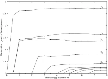
magnitudes of the estimated components change with the tuning parameterM in one run. The magnitudes of the functional components are measured by their empirical L1 norms,
defined as 1/nPn
i=1|fˆj(x(ij))|for j= 1, ..., d. The λ0 in this run is fixed at 9.7656×10⁻⁶.
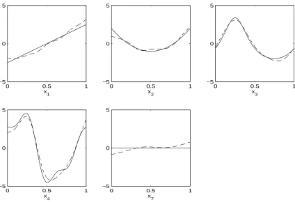
Both GCV and five-fold cross validation choose M = 3.5, giving a model of 5 terms in this run. The estimated function components are plotted along with the true function components in Figure 2. Notice the components are centered according to the ANOVA decomposition.
0 1 2 3 4 5 6 7 8
0 0.5 1 1.5 2 2.5 3
x 4
x 3
x 1
x 2
x7
The tuning parameter M
The empirical L
1
norm of the components
Figure 1: The empiricalL1norm of the estimated components as plotted against the tuning
0 0.5 1 −5
0 5
x
1
0 0.5 1
−5 0 5
x
2
0 0.5 1
−5 0 5
x
3
0 0.5 1
−5 0 5
x
4
0 0.5 1
−5 0 5
x
7
Figure 2: The estimated component functions (dashed line) and the true component func-tions (solid line) in one run of Example 1. Shown are the components for variables 1, 2, 3, 4, and 7. For the other variables, both the true and estimated component functions are zero.
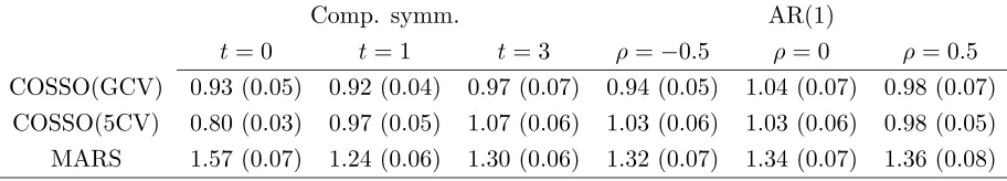
We compare COSSO with GCV, COSSO with five-fold cross validation, and MARS. The measure of accuracy is the integrated squared error ISE = EX{fˆ(X)−f(X)}2. For
Table 1. The average integrated squared errors over 100 runs of Example 1 in different settings.
Comp. symm. AR(1)
t= 0 t= 1 t= 3 ρ=−0.5 ρ= 0 ρ= 0.5 COSSO(GCV) 0.93 (0.05) 0.92 (0.04) 0.97 (0.07) 0.94 (0.05) 1.04 (0.07) 0.98 (0.07)
COSSO(5CV) 0.80 (0.03) 0.97 (0.05) 1.07 (0.06) 1.03 (0.06) 1.03 (0.06) 0.98 (0.05) MARS 1.57 (0.07) 1.24 (0.06) 1.30 (0.06) 1.32 (0.07) 1.34 (0.07) 1.36 (0.08)
To study the performance of the COSSO in terms of model selection, we determine in the uniform case the number of times each variable appears in the 100 chosen models (Table 2), and the number of terms in the 100 chosen models (Table 3). In our calculation we take θ to be zero if it is smaller than 10−6. The COSSO with five-fold cross validation
misses the second variable 6 times, but chooses the correct four variable model 84 times. The COSSO with GCV and MARS never miss any important variable, but tend to include uninformative variables in the chosen models. The COSSO with GCV chooses the correct four variable model 57 times, while MARS does that only 4 times.
Table 2. The frequency of appearance of the variables in the models chosen in 100 runs of Example 1 in the uniform setting.
Variable
1 2 3 4 5 6 7 8 9 10 COSSO(GCV) 100 100 100 100 14 11 18 15 11 13 COSSO(5CV) 100 94 100 100 1 1 3 2 4 2
MARS 100 100 100 100 35 35 34 39 28 35
Table 3. The frequency of the size of the models chosen in 100 runs of Example 1 in the uniform setting.
Model size
3 4 5 6 7 8 9 10 Mean COSSO(GCV) 0 57 17 18 5 2 0 1 4.82
COSSO(5CV) 6 84 7 3 0 0 0 0 4.07 MARS 0 4 24 40 26 6 0 0 6.06
with five-fold cross validation is close to 4, the size of the true model. The COSSO with GCV selects slightly larger models. The models chosen by MARS are even larger.
Table 4. Mean and standard deviation of the model sizes chosen in 100 runs of Example 1. Comp. symm. AR(1)
t= 1 t= 3 ρ=−0.5 ρ= 0 ρ= 0.5 COSSO(GCV) 4.8 (1.2) 4.8 (1.5) 4.7 (1.2) 4.8 (1.3) 4.6 (1.2)
COSSO(5CV) 4.1 (1.2) 4.4 (1.9) 4.1 (1.2) 4.0 (1.0) 3.8 (0.9) MARS 6.3 (0.9) 6.2 (0.9) 6.1 (1.0) 6.1 (0.8) 5.9 (0.8)
Example 2. We consider a larger additive model with d= 60. The regression function
is
f(x) = g1(x(1)) +g2(x(2)) +g3(x(3)) +g4(x(4))
+ 1.5g1(x(5)) + 1.5g2(x(6)) + 1.5g3(x(7)) + 1.5g4(x(8))
+ 2g1(x(9)) + 2g2(x(10)) + 2g3(x(11)) + 2g4(x(12)).
Therefore there are 48 uninformative variables. The sample size is 500. The variance of the normal noise is set to 0.5184, to give a signal to noise ratio of 3 : 1 in the uniform case. For comparison, in the uniform setting var{g1(X(1))} = 0.08, var{g2(X(2))} = 0.09,
var{g3(X(3))} = 0.21 and var{g4(X(4))} = 0.26. Both COSSO and MARS are run 100
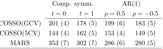
times with additive models. The results are summarized in Tables 5 and 6. We see that the two COSSO procedures outperform MARS, with the COSSO with five-fold cross validation doing slightly better than the COSSO with GCV. The COSSO(5CV) is impressive in its ability to select the correct model size: the models chosen by it all have sizes close to 12, the size of the true model.
Table 5. The average integrated squared error over 100 runs of Example 2 and its standard error, in the unit of 10−3.
Comp. symm. AR(1)
t= 0 t= 1 ρ= 0.5 ρ=−0.5 COSSO(GCV) 201 (4) 178 (5) 199 (6) 183 (5)
Table 6. Mean and standard deviation of the model sizes chosen in 100 runs of Example 2. Comp. symm. AR(1)
t= 0 t= 1 ρ= 0.5 ρ=−0.5 COSSO(GCV) 18.0 (4.1) 18.0 (4.1) 19.0 (5.1) 18.0 (4.3)
COSSO(5CV) 12.0 (0.2) 11.7 (1.4) 12.1 (1.4) 11.9 (1.0) MARS 35.2 (2.3) 36.1 (2.1) 35.2 (2.5) 35.9 (2.4)
Example 3. We consider a 10 dimensional regression problem with several two way
interactions:
f(x) =g1(x(1)) +g2(x(2)) +g3(x(3)) +g4(x(4)) +g1(x(3)x(4)) +g2(
x(1)+x(3)
2 ) +g3(x
(1)x(2)).
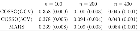
We consider the uniform setting, and set the noise to be normal with standard deviation 0.2546, to give a signal to noise ratio of 3 : 1. The average integrated squared errors are given in Table 7 for sample sizes n= 100,200,400. Both the COSSO and MARS are run with the two way interaction model. We follow the advice in Friedman (1991) to set the cost for each basis function optimization to be 3 in the MARS for two way interaction models.
Table 7. The average integrated squared error over 100 runs of Example 3 and its standard error.
n= 100 n= 200 n= 400 COSSO(GCV) 0.358 (0.009) 0.100 (0.003) 0.045 (0.001)
COSSO(5CV) 0.378 (0.005) 0.094 (0.004) 0.043 (0.001) MARS 0.239 (0.008) 0.109 (0.003) 0.084 (0.001)
There are 55 function components in the COSSO. The COSSO does not do well when
n= 100. It seems that there are too many function components for the COSSO to select from with 100 data points. MARS does not suffer from a small sample size so much as the COSSO. Part of the reason is that the MARS algorithm introduces a certain hierarchical order of the terms being searched from: only after a univariate basis function is included in the model, will the product of other terms with it become a candidate for inclusion in later steps. In contrast, the COSSO selects from all the function components and does not distinguish between main effects and interaction terms. Therefore the COSSO does not assume any hierarchical structure, and may not be efficient when the true model is hierarchical and the sample size is small. However, as the sample size increases, the COSSO procedures catch up quickly. Their performances are comparable to MARS when n= 200 and better than MARS whenn= 400.
tends to do better than the COSSO with the GCV. We therefore recommend the use of five-fold cross validation with the COSSO unless the computation time is a crucial factor.
Example 4. The circuit example. This is an example from Friedman (1991). Of interest
is the dependence of the impedanceZ of a circuit and phase shift φon components in the circuit. The true dependence is described by
Z = [R2+{ωL−1/(ωC)}2]1/2,
φ = tan−1ωL−1/(ωC)
R .
The input variables are uniform in the range
0≤R≤100,40π ≤ω≤560π,0≤L≤1,1≤C≤11,
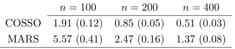
and the noise is normal with the standard deviation set to give a signal to noise level 3 : 1. This is a relatively small problem with d = 4. All order of interactions are present. Friedman (1991) applied MARS with additive model, two way interaction model, and the saturated model to this example, and found that the performance of the two way interaction model was the best. We scale the input region to [0,1]4 and apply the COSSO with five fold cross validation. With the small dimension, it is possible to apply the COSSO with the saturated model, which has 24 −1 = 15 function components. However, it turns out that the two way interaction COSSO does slightly better than the saturated model. We compare the integrated squared error of the two way interaction COSSO and that of the two way interaction MARS in Tables 8 and 9. It turns out that the COSSO performs much better than MARS.
Table 8. The average integrated squared error and its standard error for estimating the impedanceZ, in the unit of 103.
n= 100 n= 200 n= 400 COSSO 1.91 (0.12) 0.85 (0.05) 0.51 (0.03)
MARS 5.57 (0.41) 2.47 (0.16) 1.37 (0.08)
Table 9. The average integrated squared error and its standard error for estimating the phase shiftφ, in the unit of 10−3.
n= 100 n= 200 n= 400 COSSO 12.98 (0.36) 7.96 (0.20) 5.36 (0.10)
MARS 20.59 (0.96) 12.60 (0.71)1 8.19 (0.14)2
1. Excluded one extreme outlier.
8
Real examples
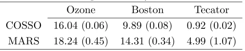
We apply the COSSO to three real datasets. They are the Ozone data, the Boston hous-ing data, and the Tecator data. The first two datasets are available from the R library “mlbench”. The Ozone data was used in Breiman and Friedman (1985), Buja, Hastie and Tibshirani (1989) and Breiman (1995). The daily maximum one-hour-average ozone reading and 8 meteorological variables were recorded in the Los Angeles basin for 330 days of 1976. The Boston housing data concerns housing values in suburbs of Boston. There are 12 input variables. The sample size is 506. The Tecator data is available from the datasets archive of StatLib at lib.stat.cmu.edu/datasets/. The data was recorded on a Tecator Infratec Food and Feed Analyzer working in the wavelength range 850 - 1050 nm by the Near Infrared Transmission (NIT) principle. Each sample contains finely chopped pure meat with differ-ent moisture, fat and protein contdiffer-ents. The input vector consists of a 100 channel spectrum of absorbances. The absorbance is−log10of the transmittance measured by the spectrom-eter. As suggested in the document, we use the first 13 principal components to predict the fat content. The total sample size is 215.
We apply the COSSO and the MARS on these datasets, and estimate the prediction squared errorsE[{Y−fˆ(X)}2] by ten-fold cross validation. We select the tuning parameter by five-fold cross validation within the training set. The estimate obtained is then evaluated on the test set. We do this ten-fold cross validation five times and then average. For all three datasets, both the COSSO and the MARS find the two way interaction model has better prediction accuracy than the additive model. Therefore we choose to apply the two way interaction model and the results are given in Table 10. We can see the COSSO does considerably better than the MARS.
Table 10. The estimated prediction squared errors and their standard errors (in parentheses).
Ozone Boston Tecator COSSO 16.04 (0.06) 9.89 (0.08) 0.92 (0.02)
MARS 18.24 (0.45) 14.31 (0.34) 4.99 (1.07)
9
Discussion
The difference between the COSSO and the common smoothing spline mirrors that between the LASSO and the ridge regression. We have shown that the COSSO has attractive properties for model selection and estimation.
of freedom for calculating the θ’s is not clear, since the θ’s are constrained instead of free parameters. This is a direction for further research.
The computation of LASSO is quite intensive for large data. The smoothing spline step in the COSSO alone requires O(n3) flops. A method that is commonly employed in the
smoothing spline method to reduce computation load is the parsimonious bases approach used by Xiang and Wahba (1996), Ruppert and Carroll (2000), Lin, Wahba, Xiang, Gao, Klein and Klein (2000) and Yau, Kohn and Wood (2002). It has been shown that the number of basis terms can be much smaller than n without degrading the performance of the estimation. It should be possible to use this approach in the COSSO estimate for large problems.
It is possible to extend the COSSO idea to other settings, such as the generalized regression, hazard regression, and density estimation. The performances of the COSSO in these settings will be studied in the future.
It is possible to construct confidence intervals and error bars for the COSSO estimate by bootstrapping. However, that is computationally very intensive. It is of interest to see to what extent the Bayesian confidence interval of the smoothing spline in Wahba (1983) and Nychka (1988) can be adapted to the COSSO.
APPENDIX 1
Proof of Theorem 1. Denote the functional to be minimized in (5) by A(f), then
A(f) is convex and continuous. Without loss of generality, we assumeτ = 1.
By (6) we have that J(f) ≥ kfk, for any f ∈ F1. Let RF1 be the reproducing kernel
of F1 and h·,·iF1 be the inner product in F1. Denote a = max n i=1R
1/2
F1 (xi, xi). By the
definition of reproducing kernel, we have for anyf ∈ F1 andi= 1, ..., n,
|f(xi)| = |hf(·), RF1(xi,·)iF1| ≤ kfkhRF1(xi,·), RF1(xi,·)i
1/2
F1
= kfkR1F/12(xi, xi)≤akfk ≤aJ(f). (A1)
Denoteρ= maxni=1(y2i +|yi|+ 1). Consider the set
D={f ∈ F :f =b+f1,with b∈ {1}, f1 ∈ F1, J(f)≤ρ,|b| ≤ρ1/2+ (a+ 1)ρ}.
Then D is a closed, convex, and bounded set. Therefore by Theorem 4 of Tapia and Thompson (1978, page 162), there exists a minimizer of (5) inD. Denote the minimizer by
¯
f. ThenA( ¯f)≤A(0)< ρ.
On the other hand, for any f ∈ F with J(f) > ρ, clearly A(f) ≥ J(f) > ρ; for any
get that, for anyi= 1, ..., n,
|b+f1(xi)−yi|>[ρ1/2+ (a+ 1)ρ]−aρ−ρ=ρ1/2.
Therefore we haveA(f)> ρ.
Hence for any f 6∈D, we have A(f)> A( ¯f). Therefore ¯f is a minimizer of (5) in F.
Proof of Theorem 2. The proof follows the approach in van de Geer (2000) and makes use of Theorem 10.2 of van de Geer (2000, page 169). For completeness we state the theorem first: (the original theorem is more general, and the following corresponds to the special case ν = 1 and Gaussian noises of the original theorem):
Lemma 3 (Theorem 10.2 of van de Geer) Consider a regression model yi =g0(xi) +
ǫi, i= 1, ..., n, where g0 is known to lie in a class G of functions, xi’s are given covariates
in [0,1]d, and ǫ
i’s are independent N(0, σ2) noises. Let I :G →[0,∞) be a pseudo-norm
onG. Define gˆ= arg ming∈G1/nPni=1{yi−g(xi)}2+τn2I(g). Assume
H∞(δ,{
g−g0
I(g) +I(g0) :g∈ G, I(g) +I(g0)>0})≤Aδ
−α (A2)
for all δ >0, n≥1 and some A >0, 0< α < 2. Here H∞ stands for the entropy for the
supreme norm. Then (i) if I(g0) > 0, and τn−1 = Op(n1/(2+α))I(2−α)/(4+2α)(g0), we have
kgˆ−g0kn=Op(τn)I1/2(g0); (ii) ifI(g0) = 0, we havekˆg−g0kn=Op(n−1/(2−α))τ
−2α/(2−α)
n .
The above lemma can not be used directly since (A2) is not satisfied in our case. This problem can be dealt with with the following arguments.
For any f ∈ F, we can write f(x) =c+f1(x(1)) +...+fd(x(d)) =c+g(x), such that
Pn
i=1fj(x(ij)) = 0, j = 1, ..., d. Similarly, write f0(x) = c0+f01(x(1)) +...+f0d(x(d)) =
c0 +g0(x), and ˆf(x) = ˆc + ˆf1(x(1)) + ...+ ˆfd(x(d)) = ˆc + ˆg(x). Then by construction
Pn
i=1{g0(xi)−g(xi)}= 0, we can write (5) as
(c0−c)2+
2
n(c0−c)
n
X
i=1 ǫi+
1
n
n
X
i=1
{g0(xi) +ǫi−g(xi)}2+τn2J(g).
Therefore, the minimizing ˆc must minimize (c0 −c)2 + 2/n(c0 −c)Pni=1ǫi. That is,
ˆ
c =c0 + 1/nPni=1ǫi. Therefore (ˆc−c0)2 converges with rate n−1. On the other hand, ˆg
must minimize
1
n
n
X
i=1
{g0(xi) +ǫi−g(xi)}2+τn2J(g).
Let G = {g ∈ F : g(x) = f1(x(1)) +...+fd(x(d)), with Pni=1fj(x(ij)) = 0, j = 1, ..., d}.
satisfied follows from Lemma 4 given below, sinceJ(g−g0)≤J(g) +J(g0) for anyg∈ G.
The conclusion of Theorem 2 then follows from the conclusion of Lemma 3.
Lemma 4
H∞(δ,{g∈ G :J(g)≤1})≤Ad3/2δ−1/2,
for all δ >0, n≥1 and some A >0 not depending onδ, n, or d.
Proof of Lemma 4. DefineGj as the set of univariate functions ofx(j):
Gj ={fj ∈S:J(fj)≤1, n
X
i=1
fj(x(ij)) = 0}={fj :{fj(1)−fj(0)}2+
Z 1
0
(fj′′)2≤1,
n
X
i=1
fj(x(ij)) = 0},
whereS is the second order Sobolev space.
First, we show that for any h ∈ Gj, we have |h|∞ ≡ {sups∈[0,1] |h(s)|} ≤ 1. Since Pn
i=1h(x (j)
i ) = 0, there exists a∈ [0,1], such that h(a) = 0. Now if h is monotone, since
h∈ Gj, we have maxh−minh=|h(1)−h(0)| ≤1, so|h|∞≤1; ifh is not monotone, then
max(h′)>0 and min(h′)<0. Now sinceh
∈ Gj, we have
1≥
Z 1
0
(h′′)2 ≥(
Z 1
0 |
h′′|)2 ≥ {max(h′)−min(h′)}2.
So −1≤min(h′)<0<max(h′)≤1. So |h′|∞≤1. Now since h(a) = 0, we have|h|∞≤1.
It then follows from Theorem 2.4 of van de Geer (2000, page 19)that
H∞(δ,Gj)≤Aδ−1/2 (A3)
for all δ >0, andn≥1, and some positive Anot depending on δ and n.
By the definition of theG andGj, we see that in terms of the supreme norm, if eachGj,
j = 1, ...d, can be covered by N balls of radiusδ, Then the set {g∈ G :J(g)≤1} can be covered byNd balls with radius dδ. By (A3) we get
H∞(dδ,{g∈ G :J(g)≤1})≤Adδ−1/2,
and the conclusion of the lemma follows.
Proof of Lemma 1. For any f ∈ F, we can write f = b+Pp
α=1fα with fα ∈ Fα.
Let the projection of fα onto span{Rα(xi,·), i = 1, ..., n} ⊂ Fα be denoted by gα, and
the orthogonal complement by hα. Then fα = gα +hα, and kfαk2 = kgαk2 +khαk2,
α = 1, ..., p. Since R= 1 +Pp
of the orthogonal structures,
f(xi) =h1 + p
X
α=1
Rα(xi,·), b+ p
X
α=1
(gα+hα)i=b+ p
X
α=1
hRα(xi,·), gαi,
whereh·,·iis the inner product inF. Therefore (5) can be written as
1
n
n
X
i=1
{yi−b− p
X
α=1
hRα(xi,·), gαi}2+τ2 p
X
α=1
(kgαk2+khαk2)1/2.
Therefore any minimizingf satisfieshα = 0, α= 1, ..., p, and the conclusion of the lemma
follows.
Proof of Lemma 2. Denote the functional in (5) byA(f), and the functional in (7) by
B(θ, f). For any α= 1, ..., p, we have λ0θ−1
α kPαfk2+λθα ≥2λ10/2λ1/2kPαfk =τ2kPαfk,
for any θα ≥ 0 and f ∈ F, and the equality holds if and only if θα = λ01/2λ−1/2kPαfk.
ThereforeB(θ, f)≥A(f) for any θα ≥0, α= 1, ..., p, and f ∈ F, and the equality holds if
and only if θα =λ10/2λ−1/2kPαfk,α = 1, ..., p. The conclusion of the lemma follows.
APPENDIX 2
Further derivations in the tensor product design case. Now we consider the function spaceF. Define Σ ={K¯(xi,1, xj,1)}m×m, the marginal kernel matrix corresponding
to the reproducing kernel of ¯T. With a little abuse of notation, letRj,j = 1,2, also stand
for then×nmatrix of the reproducing kernelRj evaluated at thendata points, and same
forR12. Suppose the data points are permuted appropriately, we haveR12= Σ⊗Σ, where ⊗ stands for the Kronecker product between matrices. See Chen (1991). Let 1m be the
column vector consisting of mones. For the main effect spaces, we have, R1 = Σ⊗(1m1Tm)
and R2 = (1m1Tm)⊗Σ.
Straightforward calculation gives Σ1m =mt1m, wheret= 1/(720m4). Let{ξ1 = 1m,ξ2,
...,ξm}be an orthonormal (with respect to the inner producth·,·im inRm) eigensystem of
Σ, with corresponding eigenvaluesmη1,mη2, ...,mηm, whereη1=t, andη2 ≥η3 ≥...≥ηm.
Then it is well known that ηi ∼ i−4, for i ≥ 2. See Utreras (1983). Notice ξ1, ξ2, ..., ξm
are also the eigenvectors of 1m1Tm, with corresponding eigenvalues being m, 0, ...,0. Write
ξµν =ξµ⊗ξν. It is then easy to check that {ξµν :µ, ν = 1, ..., m} form an eigensystem of
R1,R2, and R12. The eigenvalues ofR1,R2, andR12 are, respectively,
r1,µ1 = nηµ; r1,µν = 0 for µ≥1, ν ≥2;
r2,1ν = nην; r2,µν = 0 for µ≥2, ν ≥1;
It is clear that{ξµν :µ, ν = 1, ..., m}is also an orthonormal basis inRnwith respect to
the inner product h·,·in. Consider the vector of length n of function values at the sample
points: f = (f(xk,1, xℓ,2) :k, ℓ= 1, ..., m)T. LetO be the n×nmatrix with columns being
the vectors ξµν, µ, ν = 1, ..., m. Then OTO = nI. Denote a= (aµν : µ, ν = 1, ..., m)T =
(1/n)OT
f, and z= (zµν :µ, ν = 1, ..., m)T= (1/n)OTy. That is,
aµν =hf, ξµνin, zµν =hy, ξµνin;
thenf ∈Rn can be expanded in terms of the orthonormal basis:
f =X
µ,ν
aµνξµν =f0+f1+f2+f12,
where f0 = a11ξ11, f1 =Pm
µ=2aµ1ξµ1,f2 = Pm
ν=2a1νξ1ν, f12 = Pm
µ=2 Pm
ν=2aµνξµν. Then
all the components f0, f1, f2, f12, are orthogonal in Rn. Furthermore, we have zµν =
aµν+δµν, whereδµν ∼N(0, σ2/n), for µ≥1, ν ≥1.
Now let us consider the COSSO estimate (10):
1
n(y−Rθc−b1n)
T
(y−Rθc−b1n) +cTRθc+λ p
X
α=1
θα, subject to θα≥0, α= 1, ..., p,
whereRθ =Ppα=1θαRα. Lets=OTc,Dα= (1/n2)OTRαO. ThenDαis a diagonal matrix
with diagonal elements beingrα,µν/n,α= 1,2, or 12. The COSSO problem can be written
as
(z−Dθs−(b,0, ...,0)T)T(z−Dθs−(b,0, ...,0)T) +sTDθs+λ p
X
α=1 θα,
whereDθ=Ppα=1θαDα. It can then be shown by straightforward calculation that, for the
minimizing s,b, and θ, ˆs11= 0, ˆb=z11, and sand θ minimize
X
µ≥2
[{zµ1−ηµ(θ1+θ12t)sµ1}2+ηµ(θ1+θ12t)s2µ1]
+X
ν≥2
[{z1ν−ην(θ2+θ12t)s1ν}2+ην(θ2+θ12t)s21ν]
+ X
µ≥2,ν≥2
Therefore at the minimum, we have
ˆ
sµ1 = {1 +ηµ(θ1+θ12t)}−1zµ1, µ≥2;
ˆ
s1ν = {1 +ην(θ2+θ12t)}−1z1ν, ν≥2;
ˆ
sµν = (1 +ηµηνθ12)−1zµν, µ≥2, ν ≥2;
and θ’s minimize
A(θ1, θ2, θ12) = X
µ≥2
zµ21(1 +ηµθ1+ηµθ12t)−1+ X
ν≥2
z21ν(1 +ηνθ2+ηνθ12t)−1
+ X
µ≥2,ν≥2
zµν2 (1 +θ12ηµην)−1+λ(θ1+θ2+θ12),
subject to θ1 ≥ 0, θ2 ≥ 0, θ12 ≥ 0. We show that if f12 = 0 and nλ → ∞, then ˆθ12 = 0 with probability tending to one. The cases for θ1 and θ2 are similar. Direct calculation
gives ∂A/∂θ12 ≥ λ−U for any θ1 ≥ 0, θ2 ≥ 0, and θ12 ≥ 0, where U = tPµ≥2ηµzµ21+ tP
ν≥2ηνz12ν+
P
µ≥2,ν≥2ηµηνz2µν.
When f12 = 0, we have aµν = 0, for µ ≥ 2, ν ≥ 2, and zµ1 ∼ N(aµ1, σ2/n), z1ν ∼
N(a1ν, σ2/n) and zµν ∼ N(0, σ2/n) for µ, ν ≥ 2. Note Pµ≥2a2µ1 = ||f1||2L2,
P
ν≥2a21ν =
||f2||2L2, straightforward calculation gives E(U) =O(n
−1) and var(U) =O(n−2). Therefore
when nλ→ ∞, by Chebyshev’s inequality,
pr(U > λ)≤pr(|U−E(U)|> λ−E(U))≤var(U)/{λ−E(U)}2 →0,
Hence with probability tending to unity, U < λ, and ∂A/∂θ12>0, for θ1 ≥0, θ2 ≥0, and
θ12≥0. Therefore at the minimizer ofA, we have ˆθ12= 0, which implies ˆf12= 0.
That ˆf126= 0 with probability tending to one whenf126= 0 andλis appropriately chosen
follows from the consistency results Theorem 2 and the comments thereafter in Section 2.4.
Acknowledgments. The authors wish to thank Grace Wahba for helpful comments.
References
Bakin, S.(1999). Adaptive regression and model selection in data mining problems. Ph.D.
dissertation, the Australian National University .
Breiman, L.(1995). Better subset selection using the nonnegative garrote. Technometrics
37 373–384.
Buja, A.,Hastie, T.and Tibshirani, R.(1989). Linear smoothers and additive models (with discussion). Ann. Statist. 17 453–555.
Chen, S.,Donoho, D.andSaunders, M.(1998). Atomic decomposition by basis pursuit.
SIAM J. Sci. Comput. 2033–61.
Chen, Z. (1991). Interaction spline models and their convergence rates. Ann. Statist. 19
1855–1868.
Craven, P.and Wahba, G.(1979). Smoothing noisy data with spline functions. Numer.
Math. 31377–403.
Fan, J. and Li, R. Z. (2001). Variable selection via penalized likelihood. J. Am. Statist.
Assoc.96 1348–1360.
Frank, I. E. and Friedman, J. H. (1993). A statistical view of some chemometrics regression tools. Technometrics 35109–148.
Friedman, J. H. (1991). Multivariate adaptive regression splines (invited paper). Ann.
Statist. 19 1–141.
Gu, C. (1992). Diagnostics for nonparametric regression models with additive term. J.
Am. Statist. Assoc. 871051–1058.
Gu, C. (2002). Smoothing Spline ANOVA Models. Springer-Verlag.
Gu, C. and Xiang, D.(2001). Cross-validating non-gaussian data: Generalized approxi-mate cross-validation revisited. J. Comp. Graph. Statist. 10581–591.
Gunn, S. R.andKandola, J. S.(2002). Structural modeling with sparse kernels. Mach.
Learning 48115–136.
Hastie, T.andTibshirani, R.(1990). Generalized Additive Models. Chapman and Hall.
Knight, K.and Fu, W. J. (2000). Asymptotics for Lasso-type estimators. Ann. Statist.
28 1356–1378.
Lin, X.,Wahba, G.,Xiang, D.,Gao, F.,Klein, R.andKlein, B.(2000). Smoothing spline ANOVA models for large data sets with Bernoulli observations and the randomized GACV. Ann. Statist. 281570–1600.
Lin, Y. (2000). Tensor product space ANOVA models. Ann. Statist. 28734–755.
Nychka, D. (1988). Bayesian confidence intervals for smoothing splines. J. Am. Statist.
Ruppert, D. and Carroll, R. (2000). Spatially-adaptive penalties for spline fitting.
Australian and New Zealand Journal of Statistics 45 205–223.
Tapia, R. and Thompson, J. (1978). Nonparametric Probability Density Estimation. Baltimore, MD: Johns Hopkins University Press.
Tibshirani, R. J. (1996). Regression shrinkage and selection via the lasso. Journal of
Royal Statistical Society, B 58267–288.
Utreras, F. (1983). Natural spline functions: their associated eigenvalue problem.
Nu-meri. Math.42 107–117.
van de Geer, S. (2000). Empirical Processes in M-Estimation. Cambridge University Press.
Wahba, G. (1983). Bayesian “confidence intervals” for the cross-validated smoothing spline. J. R. Statist. Soc. B 45133–150.
Wahba, G. (1990). Spline Models for Observational Data, vol. 59. SIAM. CBMS-NSF Regional Conference Series in Applied Mathematics.
Wahba, G., Wang, Y., Gu, C., Klein, R. and Klein, B. (1995). Smoothing spline ANOVA for exponential families, with application to the WESDR. Ann. Statist. 23
1865–1895.
Wahba, G.andWold, S.(1975). A completely automatic French curve.Commun. Statist.
4 1–17.
Xiang, D.andWahba, G.(1996). A generalized approximate cross validation for smooth-ing splines with non-Gaussian data. Statist. Sinica 6 675–692.
Yau, P.,Kohn, R.andWood, S.(2002). Bayesian variable selection and model averaging in high dimensional multinomial nonparametric regression. J. Comp. Graph. Statist.To appear.
Zhang, H., Wahba, G., Lin, Y., Voelker, M., Ferris, M., Klein, R. and Klein, B. (2002). Variable selection and model building via likelihood basis pursuit. Technical