Scholarship@Western
Scholarship@Western
Electronic Thesis and Dissertation Repository
10-23-2014 12:00 AM
Censored Time Series Analysis
Censored Time Series Analysis
Nagham Muslim Mohammad
The University of Western Ontario
Supervisor Dr.A. Ian McLeod
The University of Western Ontario
Graduate Program in Statistics and Actuarial Sciences
A thesis submitted in partial fulfillment of the requirements for the degree in Doctor of Philosophy
© Nagham Muslim Mohammad 2014
Follow this and additional works at: https://ir.lib.uwo.ca/etd
Part of the Statistics and Probability Commons
Recommended Citation Recommended Citation
Mohammad, Nagham Muslim, "Censored Time Series Analysis" (2014). Electronic Thesis and Dissertation Repository. 2489.
https://ir.lib.uwo.ca/etd/2489
This Dissertation/Thesis is brought to you for free and open access by Scholarship@Western. It has been accepted for inclusion in Electronic Thesis and Dissertation Repository by an authorized administrator of
by
Nagham Muslim Mohammad
Graduate Program in Statistics and Actuarial Science
A thesis submitted in partial fulfillment
of the requirements for the degree of
Doctor of Philosophy
The School of Graduate and Postdoctoral Studies
The University of Western Ontario
London, Ontario, Canada
c
Environmental data is frequently left or right censored. This is due to the fact that the correct value for observed values that are below or above some threshold or detection point are inaccurate so that it is only known for sure that the true value is below or above that threshold. This is frequently important with water quality and air quality time series data. Interval censoring occurs when the correct values of the data are known only for those values falling above some lower threshold and below some upper threshold. Censoring threshold values may change over time, so multiple censor points are also important in practice. Further discussion and examples of censoring are discussed in the first chapter. A new dynamic normal probability plot for censored data is described in this chapter.
For some environmental time series the effect of autocorrelation is negligible and we can treat the data or often the logged data as a random sample from a normal population. This case has been well studied for more than half a century and the work on this is briefly reviewed in the second chapter. The second chapter also contains a new derivation and a new algorithm based on the EM algorithm for obtaining the maximum likelihood estimates of the mean and variance from censored normal samples. A new derivation is also given for the observed and expected Fisher information matrix.
In chapter three the case of autocorrelated time series is discussed. We show the close relationship between censoring and the missing value problem. A new quasi-EM algorithm for missing value estimation in time series is described and it efficacy demonstrated. This algorithm is extended to handle censoring in the general case of multiple censor points and interval censoring. When there is no autocorrelation, this algorithm reduces to the algorithm developed in Chapter 2. An application to water quality in the Niagara river is discussed.
Keywords: Time series analysis, censoring, environmetrics
First and foremost I would like to express my sincere gratitude to my supervisor Professor A. Ian McLeod for his invaluable guidance and generous support throughout the course of my study at Western. I would also like to thank my thesis examiners, Professors Dr. Hao Yu, Dr. Jiandong Ren, Dr. Jean-Marie Dufour and Dr. John Koval for carefully reading this thesis and helpful comments. I am also grateful to all faculty, staffand fellow students at the Department of Statistical and Actuarial Sciences for their encouragement. The author would also like to acknowledge the financial support of the Department of Statistical and Actuarial Sciences and the Faculty of Graduate Studies and the Board of the Ontario Graduate Scholarships in Science and Technology. Finally, I would like to thank my family for their patience and love that helped me to reach this point.
Abstract ii
Acknowledgements iii
List of Figures v
List of Tables vii
1 Introduction and literature review 1
2 Censored normal random samples 24
3 Censored time series analysis 49
4 Conclusions 73
Bibliography 74
Curriculum Vitae 77
1.1 Left-censoring and the corresponding right-truncated distribution. . . 2
1.2 Simple normal probability plot of some left censored simulated N(0,1) data with censor pointc=−0.5,i=1, . . . ,60. . . 3
1.3 Time series plot of simulated censored AR(2) series for the model that was fit to the cloud ceiling time series. The observed censor rate was 27.5% which was lower than the 41.62% rate in the observed historical time series. . . 4
1.4 Boxplot of the censor rate in 100 simulations of the AR(2) model fitted to the cloud ceiling time series. The dotted horizontal line shows the observed censor rate in the observed data. . . 4
1.5 A strictly convex function. . . 5
1.6 Convergence of EM and MCEM after 25 iterations with M = 100 for sample sizen=50 with censor rater= 0.5. . . 12
1.7 Comparing EM and MCEM after 25 iterations with M = 1 for sample size n=50 with censor rater=0.5. . . 12
1.8 Time series plot of 12 Dichloro in Niagara River at Fort Erie. . . 18
1.9 The probability density function using Gaussian kernel of 12 Dichloro in Nia-gara River at Fort Erie. . . 19
1.10 Log transformed 12 Dichloro . . . 19
1.11 Autocorrelation plot of Log transformed 12 Dichloro . . . 20
1.12 Diagnostic plot fitted AR(1) produced by tsdiag(). . . 21
1.13 Diagnostic plot fitted ARMA(1,1) produced by tsdiag(). . . 22
1.14 Monte-Carlo Ljung-Box test diagnostic plots for fitted ARMA(1,1). . . 22
1.15 Monte-Carlo Ljung-Box test diagnostic plots for fitted AR(1). . . 22
1.16 Autocorrelation function of the fitted ARMA(1,1) process. . . 23
1.17 Spectral density function of the fitted ARMA(1,1) process. . . 23
2.1 Boxplots comparing the estimates of the mean obtained using the EM algo-rithm and direct numerical optimization using Mathematica’s general purpose FindMaximum function. . . 29
2.2 The relative likelihood functions using the censored likelihood (solid blue) and the approximation obtained by treating the censored values as observed. In this case the censor rate was about 40 percent so the effect on the bias of the estimate is very strong. As the censor rate decreases the bias will decrease. . . . 30
2.3 The bias of the MLE and jackknife estimators for the mean and standard devi-ation are compared. . . 32
2.5 The expected information for the mean in left-censored samples of size 100. . 36
2.6 The expected joint information the mean and standard deviation in left-censored N(0,1) samples of size 100. . . 37
2.7 The expected information for the standard deviation in left-censored samples. . 40
2.8 Asymptotic variances of censored MLE for mean and standard deviation. . . 41
2.9 Asymptotic correlation between MLE estimate for mean and standard deviation in left-censored normal samples. . . 41
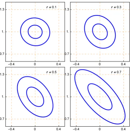
2.10 Ellipsoids of concentration corresponding to 0.95 and 0.5 probability for four censor rates. In each panel, the vertical axes corresponds to the standard devi-ation and the horizontal axis to the mean. . . 42
2.11 Comparing asymptotic standard error for MLE for mean and standard deviation with empirical estimates based on simulation. . . 43
2.12 Dynamic normal plot. . . 45
2.13 Locomotive data . . . 46
2.14 Dynamic normal plot for toxic water quality time series . . . 47
2.15 Autocorrelation functions. . . 47
3.1 The simulated latent series and the observed series with 50% missing . . . 50
3.2 Comparison of algorithms for estimating MLE in the simulated example. . . 59
3.3 Comparing RMSE for estimation of the mean. . . 60
3.4 Comparing RMSE for estimation of theϕ. . . 61
3.5 Boxplots comparing the biases for the estimates for ϕ using arima() and fi-tar()with 20 and 50 percent missing values. . . 61
3.6 Comparing RMSE for estimation of theµwith missing value rates 80% and 90% 62 3.7 Comparing RMSE for estimation of theϕwith missing value rates 80% and 90% 62 3.8 Compares the estimated standard error forµ,σˆµ, using the block with block-length 10 and parametric bootstrap in simulated CENAR(1) models with series lengthn = 200, mean zero, ϕ = −0.9,−0.6, . . . ,0.9, unit innovation variance and left censoring ratesr= 0.2, andr=0.5 . . . 65
3.9 Time series plot of simulated CENAR(1) . . . 66
3.10 Monte-Carlo test for CENARMA(1,1). . . 71
3.11 Monte-Carlo test for CENARMA(1,0). . . 71
1.1 Models fit to log 12 Dichloro time series ignoring censoring. . . 23
2.1 RMSE comparisons of Jackknife estimates with MLE. . . 32 2.2 Comparing Jackknife estimates for the standard errors with empirical
simula-tion estimates. . . 33 2.3 Comparing the asymptotic approximation for the estimated standard error of
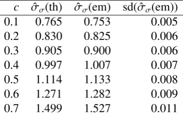
the censored MLE for mean with the estimate obtained empirically by simu-lation. The standard deviation of the empirical estimate is shown in the last column. . . 43 2.4 Comparing the asymptotic approximation for the estimated standard error of
the censored MLE for the standard deviation with the estimate obtained empir-ically by simulation. The standard deviation of the empirical estimate is shown in the last column. . . 43
3.1 Censoring process. . . 49 3.2 The estimated standard errors for estimatedµ. The first entry in each pair is for
the block bootstrap and the second for the parametric bootstrap . . . 64
Introduction and literature review
In this chapter a review is given on the underlying methods that are developed in the later chap-ters. This thesis deals with what is known as Type 1 censoring. There is an extensive literature on this subject with most of the research focused on the random sample case. The monograph by Schneider [1986] focuses on censoring with normal random samples while the monograph of Cohen [1991] discusses the more general case of random samples from normal and non-normal distributions. Wolynetz [1979a,b, 1980, 1981] has implemented Fortran algorithms for censored normal samples and censored regression. The recent monograph of Helsel [2011] provides and extensive overview of recent research with a focus on computation and censored environmental data. The seminal paper of Kaplan and Meier [1958] developed a nonparamet-ric method for fitting survival distributions with incomplete observations. Subsequently, the Kaplan-Meier curves have been widely used with times-to-event data. Very little has been done with censored time series and with the problem of fitting time series models to censored data. The paper by Park et al. [2007] is a notable exception. However as will be discussed later the algorithms and methods given in this paper are incorrect and not very useful. Hopke et al. [2001] discuss a data augmentation algorithm that is implemented to fit a non-stationary multivariate time series model to a time series of average weekly airborne particulate concen-trations of twenty four variables. The model is essentially equivalent to a vectorized version of the ARIMA(0,1,1) model.
In Chapter 2, the EM algorithm is discussed for the simple case of estimation of the mean and variance in the censored time series model consists of a mean plus Gaussian white noise. This is equivalent to the well-known and much studied problem of censored samples from a normal distribution [Cohen, 1991, Schneider, 1986, Wolynetz, 1979a] We present a new derivation using the EM algorithm as well a new closed form expression for the information matrix for the mean and variance parameters. It is shown that in the censored case these parameters are not orthogonal. A new interactive normal probability plot for censored data is discussed. Several applications are given.
Chapter 3 develops a new Quasi-EM algorithm for fitting ARMA, stationary ARFIMA and other linear time series models to censored time series. It is shown that the missing value problem in time series model fitting may be regarded as a special and extreme case of censoring and it is demonstrated that our approximate Quasi-EM algorithm handles this case just as well as the standard exact treatment. The method is illustrated with an application.
Censoring with environmental data and time series
Pollution and the monitoring of toxic substances in rivers, lakes and in the atmosphere may gives rise to samples or to time series data that are censored due to the technology used to measure the quantity of the toxic substance. Typically a sample of water or air is taken and then laboratory analysis may be used to measure the amount or concentration of the toxic substance present. The monograph of Helsel [2011] discusses statistical methods for the analysis of censored environmental data and provides many interesting environmental datasets.
The type of censoring with environmental data is known as Type 1 censoring in contrast to Type 2 censoring in which the censored observations result from stopping an experiment at a preset time.
Consider the caseZi,i = 1, . . . ,nare independent and identically distribution and the
dis-tribution function F(z) corresponds to the complete data. We do not observe Z1, . . . ,Zn but
instead we observe a censored version, denoted byYi,i=1, . . . ,n. In the case of left-censoring
Yi = max (Zi,ci),i = 1, . . . ,n where ci are the censor points or detection thresholds.
With-out loss of generality we can partition the sample (Z1,Z2, . . . ,Zn) into two parts (Y1,...,Ym)
and (Z1, . . . ,Zn−m) whereY1, . . . ,Ymcorrespond to the non-censored or complete observations
and Z1, . . . ,Zn−m correspond to the censored observations. The right-truncated distribution
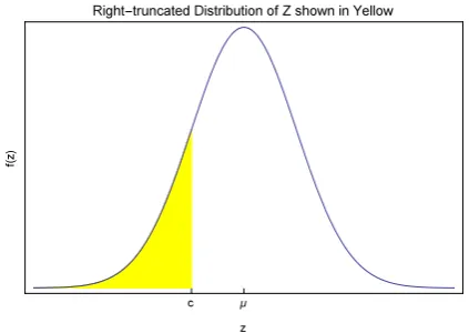
of the censored values is shown in Figure 1.1 below. Due to censoring the actual values of Z1, . . . ,Zn−mare not observed and in their place onlyYi =ci,i=m+1, . . . ,nis observed. Right
censoring is defined by setting Yi = min (Zi,ci),i = 1, . . . ,n. An important special case is
single-censoring whenc1 = . . . = cn = c. The single, left-censored normal distribution case is
shown in Figure 1.1.
Figure 1.1: Left-censoring and the corresponding right-truncated distribution.
Left-censored data or time series often arise in water or air quality applications since the in-struments may not be able to measure below or above some specified threshold,c. In this case the data may be left-censored, right-censored or if there are both upper and lower limits, inter-val censored. In lifetime data in engineering and medical sciences, right censoring of surviinter-val times is of interest [Lawless, 2003,§2.2] and we illustrate our new dynamic normal probability plot for censored data with an application to engine lifetimes that are right-censored.
is paired with a threshold value c−i,i = 1, . . . ,n so if the underlying latent process is Zi,i =
1, . . . ,n our observed process is Yi = max
(
Zi,c−i
)
,i = 1, . . . ,n in the left-censored case. It is assumed thatc−i,i = 1, . . . ,n are known. In the singly-censored case,c−i = c,i = 1, . . . ,n. Similarly in the right censored case, given c+i, we assume the unobserved latent value Zi and
we observeYi =min
(
Zi,c+i
)
,i= 1, . . . ,n. If the data is both left and right censored it is said to be interval censored. It is assumed that the censoring process that determinesci,i=1, . . . ,nis
independent of the data generation process that generates the underlying latent process,Zi,i =
1, . . . ,n. See Helsel [2011, §3.2] for more discussion and examples of the pitfalls and bias created by insider or non-independent censoring. This is not an issue with most data collected by reputable government agencies such as Environment Canada.
Simulated example
A random sample from an N(0,1) distribution of sizen= 60 was generated and all values less than−0.5 were set to−0.5. A normal probability is a useful tool for preliminary data analysis and is shown for this data in Figure 1.2. We see that there were 13 censored values, so the censor rate is 13/60 ≈ 22%. Later we will introduce a new dynamic normal probability plot that is useful for robust estimation and diagnostic checking.
Figure 1.2: Simple normal probability plot of some left censored simulated N(0,1) data with censor pointc=−0.5,i=1, . . . ,60.
Air quality example
Park et al. [2007] fit an AR(2) model,ϕ(B) (zt−µ)=at, whereϕ(B)=1−ϕ1B−ϕ2B2,Bis the
backshift operator ont,µis the series mean andatare the innovations which are assumed to be
independent and identically distributed with a normal distribution with mean zero and variance
σ2
a, to a time series of hourly cloud ceiling heights in units of 100 meters. The time series had
three missing values as well and were right censored andc= c+= 12000feet. For fitting a log transformation was used, so c = 4.79 log feet. The series was of length n = 716. The fitted model was an AR(2) with ˆϕ1 = 0.689±0.038, ˆϕ2 = 0.173±0.038, ˆµ = 4.129±0.236 and
ˆ
series plot is shown in Figure 1.3. The observed censoring rate in the fitted model was only 27.5%.
Figure 1.3: Time series plot of simulated censored AR(2) series for the model that was fit to the cloud ceiling time series. The observed censor rate was 27.5% which was lower than the 41.62% rate in the observed historical time series.
Figure 1.4: Boxplot of the censor rate in 100 simulations of the AR(2) model fitted to the cloud ceiling time series. The dotted horizontal line shows the observed censor rate in the observed data.
EM algorithm
Convex functions
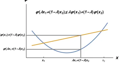
The functionφ(x) is convex on an interval (a,b) provided that
φ(λx1+(1−λ)x2)≤ λφ(x1)+(1−λ)φ(x2) (1.1)
for x1,x2 ∈ (a,b) and 0 ≤ λ ≤ 1. It is strictly convex if equality only holds when λ = 0 or λ= 1. Geometrically this means that the chord joining any two points lies above the function as shown in Figure 1.5.
Figure 1.5: A strictly convex function.
Whenφ(x) is twice differentiable, it is strictly convex onDon (a,b) if and only ifφ′′(x)> 0. The slope of the tangent is always increasing. The diagram above shows a parabola that is concave upwards. Other common examples of convex functions are exponential on (−∞,∞) and the negative of the logarithm on (0,∞).
The region above a convex function is always a convex set, that is, the line segment con-necting any two points in the region is in the region.
Jensen’s inequality
Consider a distribution with two mass points Pr{X = xi} = pi,i = 1,2. Letφ(x) be a convex
function. By definition, Eφ(X) = φ(x1)p1+φ(x2)p2 and φ(EX) = φ(p1x1+ p2x2), where E
denotes mathematica expectation.
Then Jensen’s inequality follows from the above two results and it states that,
φ(p1x1+ p2x2)≤ φ(x1)p1+φ(x2)p2 (1.2)
This proof can be extended tonpoints using mathematical induction and then it can be ex-tended to the continuous case using continuity arguments. In general, for any random variable X, ifφis any convex function for which Eφ(X) is defined then Jensen’s inequality states that,
φ(EX)≤Eφ(X) (1.3)
Illustrative example with the lognormal distribution.
Illustrative example with the lognormal distribution.Illustrative example with the lognormal distribution. Let X have a lognormal distribution with parametersµandσ2. SoY = logXis normally distributed with meanµand varianceσ2. Then it can be shown from Jensen’s inequality that E logX > µ. This follows since−logX is a strictly convex function over the positive real line, E(−log(X))>−log EXfrom eqn.(1.3) so
This result can be verified using the moment generating function for the normal distribution with parametersµandσ2. LetY be normally distributed with meanµand varianceσ2then the
moment generating function for Y is given by MY(t) = E exp(tY) = exp
{
tµ+ 12t2σ2} hence
setting t = 1, E{exp(Y)} = E{X} = exp{µ+ 12σ2} > eµ, hence EX > eµ or equivalently log EX > µ. More generally, ifY is a positive random variable, log EY ≤ E logY and equality holds only in the constant random variable case.
Kullback-Liebler discrepancy
Jensen’s inequality may be used to establish the non-negativity of the Kullback-Liebler dis-crepancy. For any two probability density functions f(x) andg(x) defined onR, the Kullback-Liebler discrepancy is defined by
K(g, f)=
∫ ∞
−∞log
f(x)
g(x) f(x)dx= Eflog f(x)
g(x) (1.4)
Proof
K(g, f)=
∫
log
(
f(x) g(x)
)
f(x)dx= −
∫
log
(
g(x) f(x)
)
f(x)dx≥ −log
∫ (
g(x) f(x)
)
f(x)dx =0
(1.5) This establishes that K(g, f)≥ 0.
Incomplete data models
By incomplete data we mean data that is possibly missing or censored. Incomplete data models are characterized by,
g(x|θ)=
∫
Z
f(x,z|θ)dz (1.6)
wherexis the observed data andzis the latent data andg() and f() are the probability density functions. As in [Robert and Casella, 2004] we use the notation g(x|θ) to mean the density function of xgivenθand similarly with others distribution functions.
Incomplete data problems also arise in other areas such as mixture models and stochastic volatility model in financial time series [Robert and Casella, 2004]
Censored data likelihood
ObservedY1, . . . ,Ynfrom IID with pdf f(y;θ). Assumey1, . . . ,ymare fully observed andym+1 = . . .= yn= care left-censored. The likelihood function is
L(θ|y)=F(c)n−m
m
∏
i=1
Letz1, . . . ,zn be latent process with zi = yi, i = 1, . . . ,mandzm+1, . . . ,zn are the observed
uncensored values. Then the complete likelihood function if we know the latent process values as well as the observed values may be written,
L(c)(θ|z)=
n
∏
i=1
f(zi;θ) = m
∏
i=1
f(yi;θ) n
∏
i=m+1
f (zi;θ) (1.8)
Then eqn. (1.7) may be written,
L(θ|y)=E{L(c)(θ|Z)} =
∫
Z
L(c)(θ|z)f (z|y1 , . . . ,ym;θ)dz. (1.9)
Note that eqn. (1.7) is of the same form as eqn. (1.9).
The EM Algorithm
In the following sections for extra precision we will use boldface to denote vectors. In later sec-tions the distinction between vector and scalars is evident from context so the use of boldface for vectors is curtailed.
Expectation equation
We supposeXi,i= 1, . . . ,mare independent and identically distributed (IID)
ˆ
θθθ= argmax
θθθ Π
m
i=1g(xi|θθθ) (1.10)
and we can write the log-likelihood,
logL(θθθ|xxx)=logg(xxx|θθθ) (1.11)
wherexxx= (x1, . . . ,xm). In practice, logL(θθθ|xxx) may be difficult or cumbersome to evaluate.
Suppose that if we augment the data withzzz= (zm+1, . . . ,zn)′where (X,Z) have PDF f(xxx,zzz|θθθ)
where f(xxx,zzz|θθθ) is easy to evaluate. The complete data likelihood,
logL(c)(θθθ|xxx,zzz)= log(f(xxx,zzz|θθθ)). (1.12)
The marginal PDF forzzzis given by
k(zzz|θθθ,xxx)= f(xxx,zzz|θθθ)
g(xxx|θθθ) (1.13)
hence,
g(xxx|θθθ)= f(xxx,zzz|θθθ)
k(zzz|θθθ,xxx) (1.14) Taking logs,
For any value ofθθθ0we can write,
Eθθθ000logL(θθθ|xxx)=Eθθθ000logL
(c)(θθθ|xxx,ZZZ,θθθ0) −E
θ0logk(ZZZ|||xxx,θθθ0). (1.16)
where Eθ0 is expectation forZZZ with respect to the distributionk(zzz|θ0 ,xxx). Since the first term does not depend onZZZ,
logL(θθθ|xxx)=Eθ0logL
(c)(θ|xxx,ZZZ)−E
θθθ0logk(ZZZ|xxx,θθθ0). (1.17)
Assume, as usual, that we can interchange expectation with respect toZZZ, and differentiation with respect toθ0,
∂θθθ0Eθθθ0logk(zzz|xxx,θθθ0) =Eθ0∂θ0logk(zzz|||xxx,θθθ0) = 0 (1.18)
where we have used the result that the expected value of the score function is zero [Casella and Berger, 2002, eq. 7.3.8]. Eqn. (1.18) shows that∂θθθ0Eθθθ0logk(zzz|xxx,θθθ0) is independent ofθθθand so
we can concentrate of maximizing E logL(c)(θ|xxx,ZZZ)
Simple illustration
This example is provided just to show in an over-simplified setting how the concepts can be apply. SupposeXi,i = 1, . . . ,mandZi,i = m+1, . . . ,nare IID normal with mean θand unit
variance.
Dropping the constant terms involving 2π,
logL(θ|xxx)=
m
∑
i=1
(
−1
2(xi−θ)
2
)
logL(c)(θ|xxx,zzz)=
m
∑
i=1
(
−1
2(xi−θ)
2
) +
n
∑
i=m+1
(
−1
2(Zi−θ)
2
)
logk(zzz|xxx, θ)=
n
∑
i=m+1
(
−1
2(Zi−θ)
2
)
First note that,
Eθ0{(Z−θ)2}=E{Z2−2θZ+θ2}
=θ2
0+1−2θθ0+θ 2
=(θ0−θ)2+1.
So we have,
Eθ0
n
∑
i=m+1
(−1
2(Zi−θ)
2
)
=−12(n−m)(1+(θ0−θ)2)
Eθ0logL(c)(θ|xxx,ZZZ)=
m
∑
i=1
(
−1
2(xi−θ)
2
)
− 1
2(n−m)
(
1+(θ0−θ)2)
and
Eθθθ0logk(ZZZ|xxx,θθθ)= −
1
2(n−m)
(
1+(θ0−θ)2).
So eqn. (1.17) is verified as correct.
EM equation
To maximize logL(θθθ|xxx) we can work with the expected log-likelihood function,
Q(θθθ|θθθ0,x)=Eθθθ0logL(c)(θθθ|xxx,zzz,θθθ0). (1.19) The iterative algorithm starts with an initial estimate ˆθθθ0 and then obtains improved esti-mates, ˆθθθ(1),θθθ(2), . . .ˆ . The improved estimates are obtained using,
ˆ
θθθ(j+1) =argmax
θθθ Q(θθθ|
ˆ
θθθ(j),xxx). (1.20)
There are two basic steps in the algorithm.
Step 1. Expectation: compute the expected value,
Eθθθ(j)logL(c)(θθθ|xxx,zzz)= Q(θθθ|θθθ(j),xxx). (1.21) Step 2. Maximization: use eqn. (1.20).
Fundamental theorem for the EM algorithm
The sequence ˆθθθ(j), j=0,1,2, . . .defined by the EM algorithm satisfies
logL(ˆθθθ(j+1)|xxx)≥logL(ˆθθθ(j)|xxx) (1.22)
with equality holding if and only if
Q(ˆθ(j+1)|θθθ(ˆ j),x)=Q(ˆθ(j)|θθθ(ˆ j),x) (1.23)
Proof
Eqn. (1.17) may be written,
logL(θθθ|xxx)= Q(θ|θθθ(ˆ j),xxx)−Eθθθ(j)logk(ZZZ|xxx,θθθ(j)). (1.24)
Hence we can write,
logL(ˆθθθ(j+1)|xxx)= Q(ˆθ(j+1)|θθθ(ˆ j),xxx)−Eθθθ(j)logk(ZZZ|||xxx,,,θθθ(j)))). (1.25)
logL(ˆθθθ(j)|xxx)= Q(ˆθθθ(j)|θθθ(ˆ j),xxx)−Eθθθ(j)logk(ZZZ|xxx,θθθ(j)). (1.26)
So we obtain,
logL(ˆθ(j+1)|xxx)−logL(ˆθ(j)|xxx)= Q(ˆθ(j+1)|θ(ˆ j),xxx)−Q(ˆθ(j)|θ(ˆ j),xxx)−Eθ(j)logk(ZZZ|||xxx,,,θ(j+1))))+++Eθ(j)logk(ZZZ|||xxx,,,θ(j)))).
Since by definitionQ(ˆθθθ(j+1)|θθθ(ˆ j),xxx)−Q(ˆθ(j)|θ(ˆ j),xxx)≥0 we see that eqn. (1.22) holds if we have
Eθθθ(j)logk(ZZZ|||xxx,θθθ(j+1))≤ Eθθθ(j)logk(ZZZ|xxx,θθθ(j)). (1.27)
Re-arranging the terms eqn. (1.27) is equivalent to,
Eθ(j)logk(ZZZ|||xxx,,,θθθ(j+1)))) k(ZZZ|||xxx,,,θθθ(j)))) ≥
0. (1.28)
The inequality in eqn. (1.28) follows from the non-negative definiteness property of the Kullback-Liebler information.
Discussion
In cases where the likelihood function is well behaved, such as for models assuming a member of the exponential family of distributions, the likelihood function has a single unique maximum and in these cases the EM algorithm is guaranteed to converge to the global MLE [McLachlan and Krishnan, 2007,§3.4].
The Fundamental Theorem of EM only guarantees that the likelihood does not decrease. Further conditions are needed to establish that it converges to a stationary point of the likeli-hood equation∂θlogL(θ|x)=0 [Boyles, 1983, Wu, 1983].
This stationary point may be a minimum, maximum or saddlepoint. In some situations it is necessary to experiment with different initial values. A simple example of a non-regular case is provided by the Cauchy distribution since the likelihood function for the location param-eter may be multimodal. The method of simulated annealing has been used in such difficult situations to try to find the global MLE [Finch et al., 1989, Robert and Casella, 2004]. Other methods such as genetic optimization or MCMC may also be useful in such cases.
Stochastic EM algorithm
It may be that the expected value Eθθθ(j)logL(c)(θθθ|xxx,zzz) = Q(θθθ|θθθ(
j),xxx) is too difficult to compute
analytically but an approximation to it can be obtained by simulation. We need to generatezzzby drawing repeatedly from the distribution k(zzz|x,θθθ(j)). The stochastic EM algorithm comprises
the following steps: Step 1:
Step 1:
Step 1: SelectMlarge enough. Setθθθ(0)to an initial parameter estimate and set j=0. Step 2:
Step 2:
Step 2:Generate a random samplezzz(i),i= 1, . . . ,Mand compute
¯
Q(θθθ|θθθ(j),x)=
1 M
M
∑
i=1
Step 3: Step 3:
Step 3: Compute update estimate
ˆ
θθθ(j+1) =argmax
θθθ
¯
Q(θθθ|θθθ(ˆ j),xxx). (1.30)
As M→ ∞, the estimates of ˆθθθ(j+1)will stochastically converge to the true MLE, ˆθθθ.
This algorithm often referred to as the Monte Carlo EM or MCEM algorithm.
Example comparing the EM and MCEM algorithms
When the complete sample PDF, f(xxx,zzz|θθθ), is a member of the exponential family, the evaluation of eqn. (1.20) or eqn. (1.30) can be simplified [Robert and Casella, 2004, p. 191]. Following Robert and Casella [2004] we consider estimation of the mean parameterθin a normal distri-bution with known variance equal to one subject to censoring. We will assume left censoring with the censor point,c, determined byc= Φ−1(r), whereris a specified censor rate. We
sup-pose thaty1, . . . ,ym are fully observed and that there aren−mleft-censored values reported.
Let ¯ybe the sample mean ofy1, . . . ,ymand we may initial set ˆθ(0) = (m¯y+(n−m)c)/nand the
EM algorithm reduces to iterating the equation,
ˆ
θ(j+1)= (m/n)¯y+(n−m)/nEθˆ(j),c{Z}. (1.31)
where Eθˆ(j),c{Z}is the expected value of a right-truncated normal random variable with mean ˆθ(j)
and truncation pointc. If we use right censoring, then we take expectations for a left-truncated normal variable. These iterations quickly converge to the true MLE, ˆθ.
For the MCEM version, we simulate z(mi)+1, . . . ,zn(i),i = 1, . . . ,M from the right truncated
normal distribution on (−∞,c) and then compute the mean to obtain ˆθ(j), as summarized in
eqn. (1.32) below,
ˆ
θ(j) =z¯(i). (1.32)
Then we compute the updated estimate,
ˆ
θ(j+1) =(m/n)¯y+(n−m)/nθ(ˆ j). (1.33)
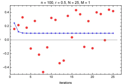
Figures 1.6 and 1.7 compare the EM and MCEM algorithms using M = 100 and M = 1 for the number of Monte-Carlo simulations. In these simulations the sample size wasn = 50 with a 50% left-censoring rate. We usedN = 25 EM iterations for both the regular EM and the Monte-Carlo EM. The blue dots, which are connected by line segments, show the EM iterations using eqn. (1.31) while the red dots show the MCEM iterations using eqn. (1.32)and(1.33) with M = 100 simulations at each iteration. In Figure 1.6 the convergence is much slower in the Monte-Carlo since it only converges stochastically as both M → ∞ and N → ∞. Observe also that the convergence in the Monte-Carlo case is non-monotonic whereas the Fundamental Theorem of EM guarantees monotonic convergence in the deterministic case.
Figure 1.6: Convergence of EM and MCEM after 25 iterations withM = 100 for sample size n=50 with censor rater= 0.5.
Park et al. [2007] propose a stochastic EM algorithm for fitting ARMA models to censored time series. However in their data augmentation, they use only M = 1. Hence the algorithm, as described in their paper, can not be expected to give sensible results. Increasing M in this algorithm would make the computations involved very laborious. At each iteration, the Gibbs algorithm of Robert [1995] for simulating from a truncated multivariate distribution is used and this Gibbs algorithm, like most MCMC methods, does not have any obvious stopping rule. Instead in Chapter 3 we propose a computational efficient quasi-EM method. In the early days of data augmentation some authors used only one simulation but informed researchers no longer do to this.
Oakes theorem
For completeness a derivation following the method described by Oakes [1999] is provided with some additional explanations. We drop the bold face notation used in the previous sections for vectors since it is clear when a variable is scalar or vector from the context. Also following Oakes [1999] we shall use the notationθandθ′to denote the values of the parameters in the EM algorithm with θbeing the current estimated parameter and θ′ the parameter to be optimized over and matrix transpose will be denoted by a superscriptT. Our derivation is essentially the same as in Oakes [1999] but a few more details and explanations are given.
In Chapter 2, we use Oakes theorem to derive a new result for the observed and expected information in random samples from a normal population.
Oakes [1999] provides an convenient algorithm for computing the information matrix for the parameters when the EM algorithm is used. Other methods have been discussed but Oakes [1999] provides a simple expression for the Hessian in terms of the objective functionQ(θ′|θ) used in the EM algorithm. We will use Oakes theorem to derive a new expression for the observed and expected information matrix in censored normal samples in Chapter 2.
Oakes theorem states that the Hessian matrix is given by,
∂2L(θ,y) ∂2θ =
{
∂2Q(θ′|θ) ∂θ′2 +
∂2Q(θ′|θ) ∂θ′∂θ
}
θ′=θ (1.34)
and so the information matrix is,
I(θ)= −
{
∂2Q(θ′|θ) ∂θ′2 +
∂2Q(θ′|θ) ∂θ′∂θ
}
θ′=θ (1.35)
Remark 1:
Remark 1:Remark 1: The covariance matrix of the MLE estimate ˆθ is I−1(θ) which in practice is
estimated byI−1(θˆ).
Remark 2:
Remark 2:Remark 2:I(θ) is the observed information. For models in the exponential family, Efron and Hinkley [1978] showed that the observed information matrix provides more accurate esti-mates of the standard errors than the expected information matrix E{I(θ)}.
Derivation DerivationDerivation
L(θ′,y)= Q(θ′|θ)−EX|Y,θlogk
(
As in the usual regularity conditions for MLE we assume that the expectation and diff eren-tiation can be interchanged, so that we can use the fact that the expected value of the score function is zero,
EX|Y,θ
∂logk(x|y, θ)
∂θ = 0 (1.37)
For the MLE, the Hessian is equal to the negative of the product of the score function,
EX|Y,θ
∂2logk(x|y, θ)
∂θ2 = −EX|Y,θ
(
∂logk(x|y, θ)
∂θ
) (
∂logk(x|y, θ)
∂θ
)T
(1.38)
Taking first derivatives in eqn. (1.36),
∂L(θ′,y)
∂θ′ =
∂Q(θ′|θ)
∂θ′ −EX|Y,θ
∂logk(x|y, θ)
∂θ′ (1.39)
From eqn. (1.37), the last term vanishes when θ′ = θ and hence the score function for the observed data,
∂L(θ′,y)
∂θ =
(
∂Q(θ′|θ)
∂θ′
)
θ′=θ (1.40)
Differentiating in eqn. (1.39) with respect toθ′
∂2L(θ′,y) ∂θ′2 =
∂2Q(θ′|θ)
∂θ′2 −EX|Y,θ
∂2logk(x|y, θ)
∂θ′2 (1.41)
Noting that,
∂2L(θ′,y)
∂θ′∂θ =0 (1.42)
Hence differentiating, in eqn. (1.39) with respect toθ
0= ∂
2Q(θ′|θ)
∂θ′∂θ −EX|Y,θ
(
∂logk(x|y, θ)
∂θ
) (
∂logk(x|y, θ)
∂θ
)T
(1.43)
Adding eqns. (1.41) and (1.43) and then using (1.42), eqn. (1.35) is obtained.
Standard errors using the jackknife
of the standard errors obtained using the Fisher information matrix method with the more computational intensive method using the jackknife.
Miller (1964) provides a review of the jackknife method and brief overview of its history. The original idea was in a paper by Quenouille in 1949 who proposed a method for removing the bias in the estimation of serial correlation and it was later extended by Tukey in 1956. Tukey introduced the terminology jackknife to indicate that this was a method of wide applicability. In modern practice, the bootstrap provides a similar computationally intensive method that is more generally applicable to statistical inference problems. In Chapter 2 we use the jackknife to compare our asymptotic standard deviations with the jackknife estimates while in Chapter 3 the bootstrap is used.
Let X = (X1, . . . ,Xn) be a sample and letgn(X) be an estimator ofθ. Tukey defined theith
pseudo-value ofgn(X) is defined to be
ui(X)=ngn(X)−(n−1)gn−1(X[i]) (1.44)
whereX[i]isXwith theith value removed. Thenui(X) is a bias corrected version ofgn(X). using
theith observation. The jackknife treatsui =ui(X),i= 1, . . . ,nasnindependent estimators of
θ. Let ¯uands2udenote the usual sample mean and variance ofui,i= 1, . . . ,n, that is,
¯ u= n−1
n
∑
i=1
ui (1.45)
and
s2u = 1 n−1
n
∑
i=1
(ui−u)¯ 2. (1.46)
Then the bias-corrected estimate ofθis,
ˆ
θ(J) =u¯ (1.47)
and the estimated standard error for both ˆθand ˆθ(J)is
est.sd(θˆ)= s2u/n. (1.48)
The jackknife 95% confidence interval is
¯
u±1.96su/ √
n. (1.49)
Tukey suggested replacing 1.96 in eqn. (1.49) by the upper 2.5% point from a t-distribution onn−1 degrees of freedom and this may be useful whennis not large. In general using the jackknife estimate forθremoves the order 1/nterm in the expansion,
E{gn(X)}=θ+ a1/n+O
(
Conditional multivariate normal distribution
LetZ be a vector of lengthn1+n2and letZ =
(
Z′1,Z2′) be a partitioned vector withZ1andZ2
of lengthsn1 andn2. Suppose thatZ is multivariate normal with mean vectorµ =
(
µ′
1, µ′2
)
and covariance matrix
Ω = (
Ω1,1 Ω1,2
Ω2,1 Ω2,2
)
(1.51)
whereΩ2,1= Ω′1,2. Then the conditional distribution ofZ2givenZ1= z1is normal with mean µ2|1 = µ2+ Ω2,1Ω1−,11(z1−µ1) (1.52)
and covariance matrix
Ω2|1= Ω2,2−Ω2,1Ω−1,11Ω1,2 (1.53)
The conditional mean in eqn. (1.52) and conditional covariance matrix in (1.53) do not require the normal assumption and hold under the assumption that theZ, Z1, andZ2 have the
covariance matrix given in eqn. (1.51).
The provides a direct method for solving the missing value problem in stationary time series. As we shall see the missing value problem is a special case of the censoring problem and this connection will be utilized.
Time series models
Let zt,t = 1,2. . . be a stationary and ergodic time series with mean µ and autocovariance
function γk = Cov (zt,zt−k). Given an observed series of length n, the covariance matrix of
(z1, . . . ,zn)′is given by
Γn =
(
γi−j
)
, (1.54)
where the (i, j)-entry in then×nmatrix is indicated. The general linear process (GLP) model may be defined by,
zt =µ+at +ψ1at−1+ψ2at−2+. . . (1.55)
whereat,t = 1,2, . . .is a sequence of independent normal random variables with mean zero,
varianceσ2aand∑kψ2k <∞.
For many parametric linear time series, ψk,k = 0,1, . . . are functions of a p-dimensional
parameter vector β ∈ Rp. An important example is the stationary and invertible ARMA(p,q)
model,
zt −µ=ϕ1(zt−1−µ)+...+ϕp
(
zt−p−µ
)
+at−θ1at−1−. . .−θqat−q (1.56)
whereat ∼IID
(
0, σ2
a
)
.In operator notation,ϕ(B) (zt−µ)=θ(B)at,whereϕ(B)=1−ϕ1B−. . .−
be written,ϕ(B)zt =ζ+θ(B)at, whereζis the intercept parameter isζ= ϕ(1)µ.The stationary
and invertible requirement may be stated that all roots of the polynomial equationϕ(B)θ(B)=0 lie outside the unit circle whereBin this equation is a complex variable. More generally we also interest in the stationary and invertible autoregressive fractionally integrated moving average ARFIMA(p,d,q) where the model equation may be written, ∇dϕ(B)z
t = ζ + θ(B)at, where |d|<1/2 andϕ(B) andθ(B) are defined as in the ARMA case.
Some important special case are whenq= 0, we have the family of autoregressive models denoted by AR(p). Similarly whenp= 0, we have the moving average process that is denoted by MA(q).
Many software packages follow another convention were the moving average component is written,θ(B)=1+θ1B+. . .+θqBqand so we must simply take the negative of the estimated
MA-coefficients.
Given data,z=(z1, . . . ,zn)′, the log-likelihood for this model may be written,
logL(β, µ, σ2a;z)= −0.5 log (det (Γn))−0.5(z−µ)′Γn−1(z−µ). (1.57)
In practice, in most cases, as discussed in McLeod et al. [2007, eqns 10-11], it is convenient to work with the concentrated log-likelihood function,
logLc(β;z)=−0.5nlog(S(β)/n)−0.5gn (1.58)
where
S(β)=
n
∑
t=1
(zt−zˆt)2
σ2
t
(1.59)
where ˆzt andσ2t are the conditional mean and variance ofztgivenz1, . . . ,zt−1and
gn = n
∑
t=1
log(σ2t). (1.60)
The innovation variance estimate is ˆσ2
a = S
(
ˆ
β)/n.
McLeod et al. [2007] discussed an R package ltsa (McLeod et al. [2012]) for the efficient computation of the log-likelihood function in eqn. (1.58) for a wide class of linear time series. Maximum likelihood estimates may be obtained by using a suitable non-linear optimizer such as provided by the R function optim() orMathematica’s FindMinimum[].
After fitting the model it is important to check the adequacy of the model assumptions. The most important assumption for our models is that the innovation sequenceat,t = 1, . . . ,n
should be approximately normally distributed and statistical independent. Moderate departure for normally are usually not important provided that the distribution is symmetric and the tails are not too heavy. But lack of independence may result in incorrect inferences and sub-optimal forecasts. A basic test for lack of independence is the Box-Ljung portmanteau test,
Qm=n(n+2) m
∑
k=1
ˆ
where ˆrk denotes the autocorrelation at lagkof the residuals, ˆat,t= 1, . . . ,nassuming the data
series is of lengthn. Under the assumption of model adequacy,Qm ∼ χ2m−p−qand large values
of Qm indicate model inadequacy. In R, a plot is constructed shown the p-value of Qm for
m=1,2, . . . ,M, whereMis a pre-selected maximum lag.
A water quality application
Dr. Abdel El-Shaarwai provided through Environment Canada some a special water quality time series that is of great practical interest. The time series is from Station ON02HA0019 (Fort Erie) on the water quality of the Niagara River. There are more than 500 water quality parameters or variables of interest in this river. The water quality in this river is monitored by a joint U.S./Canada committee. One important toxic variable of great interest is a chemical known as 12-Dichloro which when dissolved in water is measured in units of ng/L. We use a portion of the recent data on this variable that was measured approximately every two weeks over the period from March 1, 2001 to March 22, 2007. This period was chosen because it is the most recent period over which we have a time series of approximately biweekly observa-tions. The time series plot in Figure 1.8 plots the Julian day number defined so that Julian day number 1 corresponds to the date of the first observation (March 1, 2001). The 123 blue points correspond to full observations while the 21 red ones are left-censored. In total there are 144 values shown in the plot. The observed censoring rate isr =21/144=14%. The red line at the bottom indicates the detection level. After March 24, 2005 the detection level for 12 Dichloro dropped from 0.214 to 0.0878. After this change there was only one censored value at Julian day number 1807. Before the change in censoring there were 75 complete observations and 20 censored ones while from March 24, 2005 to the last observation on March 22, 2007 there were 48 complete observations and only one censored observation. It is evident from the time series plot that the data distribution is positively skewed the autocorrelations are not large. Also note change in detection level on March 24, 2005 and the apparent increase after the change. We need to be careful though since it is possible this change could be simply due to autocorrelation effect since there is no prior reason to suspect the change in detection level was related to the apparent increase in toxic level of 12-Dichloro.
This time series is available in our R package cents.
One approach could involve treating these gaps as missing values but due to the weak auto-correlation in the data this approach would not be expected to produce much improvement. So as an approximating we regard the series as successive measurements spaced approximately every two weeks with a few longer spacing. As a first approximation we ignore the censoring and treat the censored values as actual observations. Figure 1.9 shows an estimate of the prob-ability density function using Gaussian kernel with the bandwidth chosen by cross-validation. The plot shows that the data has a skewed distribution similar to a log-normal or gamma.
The sample skewness g1 = 2.76, kurtosisg2 = 13.12 and shape of the distribution are in
Figure 1.8: Time series plot of 12 Dichloro in Niagara River at Fort Erie.
coefficients are always larger in the log-normal distribution. We will proceed to analyze the logarithms of the 12 Dichloro.
The boxplot shown below shows that log transformed data is more symmetric but there is still some evidence of right skewness. The skewness and kurtosis coefficients have been reduced tog1= 0.69 andg2 =3.80 in the logged series.
Figure 1.10: Log transformed 12 Dichloro
The autocorrelation plot reveals that the autocorrelations are quite small with, r1 = 0.315
andr2 =0.220. The red-lines in the plot below indicate 95% benchmark limits estimated using
Bartlett’s large-lag formula [Box et al., 2008].
var (rk)=
(
1+ρ21+ρ22)/n (1.62)
The autocorrelation plot, Figure 1.11, reveals that the autocorrelations are quite weak. This plot suggests that AR(1) might not be the best model. Either an MA(2) or ARMA(1,1) would likely produce a better fit.
Figure 1.11: Autocorrelation plot of Log transformed 12 Dichloro
14% is not high, this approximation seems not unreasonable. The panel below shows the R script used for fitting an AR(1) and ARMA(1,1) model. The diagnostic plots in the Figures 1.13 and 1.12,suggest the AR(1) is borderline adequate while the ARMA(1,1) is completely satisfactory.
The display below shows the fitting the naive ARMA(1,1) model to the logarithms of the 12 Dichloro time series.
> require("cents") > Zdf <- NiagaraToxic > z <- log(Zdf$toxic)
> iz <- c("o", "L")[1+Zdf$cQ]
> #AR(1)
> ans <- arima(z, order=c(1,0,0)) > ans
Call:
arima(x = z, order = c(1, 0, 0))
Coefficients:
ar1 intercept 0.2889 -0.9468
s.e. 0.0798 0.0574
sigmaˆ2 estimated as 0.2408: log likelihood = -101.86, aic = 209.73
> #ARMA(1,1)
> ans <- arima(z, order=c(1,0,1)) > ans
Call:
arima(x = z, order = c(1, 0, 1))
Coefficients:
ar1 ma1 intercept
0.9152 -0.7380 -0.9043
s.e. 0.0903 0.1553 0.1251
sigmaˆ2 estimated as 0.2241: log likelihood = -96.83, aic = 201.66
borderline. In interpreting this plot it must be borne in mind that the successive p-values are not all statistically independent and are in fact very highly correlated.
Figure 1.12: Diagnostic plot fitted AR(1) produced by tsdiag().
Figure 1.13: Diagnostic plot fitted ARMA(1,1) produced by tsdiag().
For diagnostic checking CENARMA models, we recommend the Monte-Carlo test ap-proach (Lin and McLeod, 2000; Mahdi and McLeod, 2000). A script for the Monte-Carlo test is given in the documentation of the NiagaraToxic variable in the cenarma package. For comparison, the Monte-Carlo diagnostic plots for the and ARMA(1,1) and AR(1) using the Ljung-Box statistic are shown in Figures 1.14 and 1.15 and we conclude that they agree with the asymptotic test results.
From the autocorrelation plot, an ARMA(1,1) was suggested and indeed it was found that this model gave the best fit in terms of AIC as well as being adequate in terms of the port-manteau diagnostic check. The estimated parameters where ˆϕ1 = 0.9152 ± 0.0903, ˆθ1 = 0.7380 ± 0.1553, ˆµ = −0.9043 ± 0.1251, and ˆσ2
a = 0.2299. Note that when fitting with
Figure 1.14: Monte-Carlo Ljung-Box test diagnostic plots for fitted ARMA(1,1).
adjusted the answer to reflect this. A second point to note that the parameter µrefers to log 12−Dichloro.
Various other models were examined and their performance is summarized in Table 1.1.
Model AIC Portmanteau Diagnostic
ARMA(1,1) 201.66 satisfactory ARMA(2,0) 205.13 satisfactory ARMA(0,3) 207.60 satisfactory ARMA(0,2) 209.48 borderline ARMA(1,0) 209.73 failed
Table 1.1: Models fit to log 12 Dichloro time series ignoring censoring.
It is interesting that the fitted ARMA(1,1) model implies that although the autocorrelations are small, they decay quite slowly so the series has in a sense a longer memory than the other models in the above table. This series is also well fit by a stationary ARFIMA(0,1,0) model using the software Veenstra and McLeod [2014]. This longer memory is reflected in the the-oretical autocorrelation and power spectral density plots for the fitted ARMA(1,1) in Figures 1.16 and 1.17.
Figure 1.16: Autocorrelation function of the fitted ARMA(1,1) process.
Censored normal random samples
Introduction
Before developing an EM algorithm for fitting censored linear time series model we first dis-cuss the simpler case of estimating the parametersµandσ2in random samples from a normal
distribution with meanµand varianceσ2, that is, for random samples from the NID(µ, σ2)
dis-tribution. This algorithm is used to provide initial estimates of the mean in the EM algorithm that is developed for the linear model case.
A new derivation of the EM algorithm for maximum likelihood estimation (MLE) for left and right censored data with multiple censor points. The main new result in this Chapter is an explicit formula is derived for the expected and observed Fisher information matrix and it is shown that the expected information matrix gives new insight into the statistical behavior of the MLE estimates.
Another new developments is the dynamic normal probability plot of robust estimation and diagnostic checking for censored samples,
The Chapter concludes with an application to the well-known electronic locomotive en-gines dataset as well as the toxic water quality on 12 Dichloro in the Niagara river discussed in Chapter 1.
Censored sample distribution function and likelihood
Consider the more general left-censored case with latent process (Zi,ci),i = 1, . . . ,n where
Zi,i = 1, . . . ,n are independent and identically distributing with probability density function
f(z;θ) and cumulative distribution function F(z;θ), whereci,i =1, . . . ,nare known constants
or if random they are assumed to be known and to be statistically independent ofZi,i=1, . . . ,n.
If censoring is not applicable we setci = −∞for those observations for which there is no censor
point. Hence, in general, the observed process consists of some fully observed values for which Zi >ci and some censored values for whichZi ≤ ci.
Without loss of generality we may re-order the observations so the first m correspond to fully observed values, Yi,i = 1, . . . ,m. Taking into account that number ways the m
fully-observed values can be selected the probability density function for the random sample may be written,
fL(y1, . . . ,ym;θ)=
(
n m
)∏m
i=1
f (yi;θ) n
∏
i=m+1
F(ci;θ). (2.1)
The corresponding log-likelihood, after dropping the constant term, may be written,
logL(θ|y,m)=
m
∑
i=1
log f(yi;θ)+ n
∑
i=m+1
logF(ci;θ). (2.2)
In the single-left-censored case with detection levelcand parametersθ= (µ, σ),
fL(y1, . . . ,ym,|µ, σ,c,m)=
(
n m
)
F(c;µ, σ)n−m
m
∏
i=1
f(yi;µ, σ) (2.3)
and the log-likelihood function may be written,
logL(µ, σ|y,m)=(n−m) logF(c;µ, σ)+
m
∑
i=1
log f(yi;µ, σ). (2.4)
Eqn. (2.2) is equivalent to the expression given by Cohen [1991, eqn. 1.5.3] and Lawless [2003].
If censoring is ignored and we only consider the m fully observed values then Yi,i =
1, . . . ,mare distributed from a left truncated normal distribution with truncation pointsci,i =
1, . . . ,m and similarly the unobserved latent random variables Zm+1, . . . ,Zn are from a right
truncated normal distribution with truncation points cm+1, . . . ,cn. In the latent probability
model involving X1, . . . ,Xn with left-censoring atc, the number of complete observations, M,
is a random variable andm= E{M}=n(1−F(c;µ, σ)). The observedmplays the role of an an-cillary statistic and this should be taken into account for statistical inferences on the parameters
µandσ.
If the distribution is symmetric, as in the case of the normal distribution, f(yi;µ, σ) =
f(−yi;−µ, σ) and F(c;µ, σ) = 1−F(−c;−µ, σ). Consequently we see that, from a
computa-tional viewpoint, the algorithms we develop for the left-censored Gaussian case may be used with right-censoring simply be negating the data and then transforming the estimates back to the original data domain, that is, by negating them again.
In the most general case we allow multiple left and right censor points so ci =
(
c−i , c+i), wherec−i andc+i denote the left and right censor points respectively. Settingc+i = ∞means that there is no censor point for theith observation. In practice the most common situation is where there is a single censor point. For left-censoring this means,ci = (c,∞),i= 1, . . . ,n.
Maximum likelihood estimation
Left-censored normal random samples
In the first instance we consider singly left-censored data withc = c−i,i = 1, . . . ,n. Approx-imate maximum likelihood methods, using tables and charts, for estimating µand σ2 in the case of the normal distribution were given by Gupta [1978]. The log-likelihood function can be written,
L(θ|y)=(n−m) logΦ(cz)−(m/2) log
(
σ2)−(1/2)
m
∑
i=1
(yi −µ)2/σ2 (2.5)
where Φ is the standard normal CDF andcz = (c− µ)/σ. In computing environments such
as Mathematicaand R, the likelihood function may be maximized numerically using a general purpose built-in optimizer. The maximum likelihood equations are somewhat complex. Taking the first derivatives,
∂L
∂µ =(n−m)ϕ(cz) (−1/σ)/Φ(cz)+ m
∑
i=1
(yi−µ)/σ2 (2.6)
∂L
∂σ2 =(n−m)ϕ(cz) (−1)(c−µ)
/
σ2Φ(c
z)+(m/2)
/
σ2 +(1/2)
m
∑
i=1
(yi−µ)2/σ4 (2.7)
Setting∂L/∂µ=0 we obtain the first MLE equation,
ˆ
µ+σˆ(1−n/m)Ψ(cz)=y¯, (2.8)
whereΨ(z)= ϕ(z)/Φ(z). Eqn. (2.8) indicates that the mean of the left-truncated observations, ¯
y, is approximately equal to the true population meanµplus an upward adjustment that depends on the truncation point. Next setting∂L/∂σ2 =0 and simplifying,
nµ(2¯y−µ)+(n−m)σ(c−µ)Ψ((c−µ)/σ)+mσ2 =ny¯+mσˆ2y (2.9)
where ˆσ2
y = m−1
∑
i(yi−y)¯ 2. Cohen (1950, 1991) and Schneider (1986) obtained the
max-imum likelihood estimations by solving these equations iteratively but this method does not always converge since convergence depends on the initial starting values. Wolynetz (1979) pro-vides an iterative algorithm for solving the likelihood equations ∂L/∂µ = 0 and∂L/∂σ2 = 0
in the more general case with multiple left and right censor points. But since his algorithm works directly with the likelihood equations, it is not equivalent to the EM algorithm but rather a variation of the iterative algorithms discussed by Cohen (1950, 1991) and Schneider (1986). The EM algorithm, discussed next, has the advantage over the iterative methods that it always converges.
Derivation of the EM algorithm for left-censoring with normal distribution
We assume a random sampley1, . . . ,yn has been observed from a left-censored normal
and standard deviation in the underlying normal distribution without censoring. We will de-note arbitrary values of the parameters byµ′andσ′. Without loss of generality we assume that y1, . . . ,ymare not censored and thatym+1 = . . . = yn = care left-censored. We introduce latent
random variables,Zm+1, . . . ,Zn which represent the unknown values corresponding to the
cen-sored observations. ThenZm+1, . . . ,Znare a random sample of sizen−mfrom a right-truncated
normal distribution defined on (−∞,c) and with parametersµandσ. After dropping constant terms, the complete likelihood can be written,
Lc(µ′, σ′|y,z)=σ−n m
∏
i=1
exp{−(yi−µ)2/(2σ2)} n
∏
i=m+1
exp{−(zi−µ)2/(2σ2)} (2.10)
The next step is to computeQ(µ′, σ′|µ, σ,y)=EZ{logLc(µ′, σ′|y)}. We obtain,
Q(µ′, σ′|µ, σ,y)=−n
2log((σ
′)2
)− 1 2
m
∑
i=1
(yi−µ′)2/(σ′)2−
1 2
n
∑
i=m+1
EZ{(Zi−µ′)2}/(σ′)2 (2.11)
Simplifying, we may re-write this as,
Q(µ′, σ′|µ, σ,y)=−n 2log
((σ′)2)− (σ′)−2
2
m
∑
i=1
(
yi−µ′
)2+(n−m)E
Z{(Z−µ′
)2}
(2.12) ∂Q ∂µ′ =σ− 2 m ∑
i=1
(
yi−µ′)+(n−m)EZ(µ,σ,c){(Z−µ′)} (2.13)
Setting∂Q/∂µ′ = 0 and solving for ˆµ,
0= m¯y−mµˆ+(n−m)Ez{Z} −(n−m) ˆµ
0=my¯+(n−m)Ez{Z} −nµˆ. Hence,
ˆ
µ= (m/n)¯y+(n−m)/nEz{Z}. (2.14)
Using Mathematica, we obtain the expectation in the right-truncated distribution,
EZ{Z|µ, σ,c}=
µerf
(
c−µ
√ 2σ ) − √ 2
πσe−
(c−µ)2 2σ2 +µ
/erfc
(
µ−c
√
2σ
)
(2.15)
where erf(z) is the error function defined for z ≥ 0 as erf(z) = √2
π
∫z
0 e
−t2
∂Q
∂(σ′)2 = −
n(σ′)−2
2 +
(σ′)−4 2 m ∑
i=1
(
yi−µ′
)2+(n−m
)EEµ,σ,c
{(
Z−µ′)2}. (2.16)
Setting∂Q/∂(σ′)2 = 0 and solving
ˆ
σ2 =
n−1
m
∑
i=1
(yi−µˆ)2+(n−m)Eµ,σ,c
{
(Z−µˆ)2} (2.17)
where, using Mathematica,
EZ
(
Z−µ′)2 =
−e−(c−2σµ2)2 √
2
πσ
(
c+µ−2µ′)+
(
1+erf
[
c−µ
√
2σ
]) (
µ2+σ2−2µµ′+(µ′)2)
/erfc
[
−c+µ
√
2σ
]
(2.18)
Combining eqns. (2.14) and (2.17), the EM algorithm for computing the MLE can now be written. We start with initial estimates ˆµ(0) and(σˆ2)(0) that may, in general be obtained by
replacing the censored values with the corresponding censor point or perhaps some suitable value or values.
Algorithm CM1. Algorithm CM1.
Algorithm CM1. Singly left-censored samples.
Step 1: Initialization: j←−0 andMaxiter←−100
Step 2: µ˜z←−Eµˆ(j),σˆ(j),c{Z}
Step 3: µˆ(j+1) ←−(m/n)¯y+(n−m)/nµ˜
z
Step 4: Compute ˜σ2
z ←−Eµˆ(j),σˆ(j),c {
(Z−µ)2}
Step 5: (σˆ2)(j+1)←−n−1{∑im=1(yi−µˆ)2+(n−m) ˜σ2z
}
Step 6: Test for convergence of the estimates. If they have not converged, j ←− j+1 and repeat Steps 2-5 provided that j<MaxIter.
Remarks RemarksRemarks
1. The EM algorithm can be robustified by replacing the sample mean by some other robust estimator of location. As well a robust estimate for the ∑mi=1(yi−µˆ)2 could also be
introduced. Various state-of-the-art robust estimators for location and scale are available in R Venables and Ripley [2002].