Slender-Body Hypervelocity Boundary-Layer Instability

(1)

Instability

Thesis by

Nick Parziale

In Partial Fulfillment of the Requirements

for the Degree of

Doctor of Philosophy

California Institute of Technology

Pasadena, California

2013

(2)

Nick Parziale

(3)

(4)

Abstract

With novel application of optical techniques, the slender-body hypervelocity

boundary-layer instability is characterized in the previously unexplored regime where

thermo-chemical effects are important. Narrowband disturbances (500-3000 kHz) are

mea-sured in boundary layers with edge velocities of up to 5 km/s at two points along the

generator of a 5 degree half angle cone. Experimental amplification factor spectra

are presented. Linear stability and PSE analysis is performed, with fair prediction

of the frequency content of the disturbances; however, the analysis over-predicts the

amplification of disturbances. The results of this work have two key implications: 1)

the acoustic instability is present and may be studied in a large-scale hypervelocity

reflected-shock tunnel, and 2) the new data set provides a new basis on which the

(5)

Acknowledgements

Firstly, I would like to thank Joe Shepherd and Hans Hornung for the opportunity

they afforded me in pursuing an advanced degree at Caltech. It was a privilege to

work with them. They are accomplished scientists with “big” personalities; this made

the work particularly rewarding because of the fun we had solving problems.

Without Bahram Valiferdowsi, the quality of the work reported here would be

comprised. Working with Bahram to make several key improvements to the

tunnel-operation procedure helped make the experiments far more repeatable. I thank

Bahram for more than his technical and engineering support, he is a close friend

and it has been my pleasure to work with him.

I would like to thank Joe Jewell, my lab mate in T5. I have learned about

many things from Joe, ranging from science to wine. His suggestions, efforts, and

friendship have most certainly improved the quality of the work reported here, and

my overall experience at Caltech. I would also like to thank Ivett Leyva for her

support (including molybdenum nozzle throats and optical table legs) and friendship

during my time at Caltech. Ross Wagnild of Sandia National Laboratories helped get

the software package “STABL” running and provided valuable insight into

boundary-layer stability calculations.

I would like to thank Guillaume Blanquart and Beverly McKeon for sitting on

my thesis committee and the time they spent reviewing the work. In addition, Ravi

Ravivhandran has been a mentor to me during my time at Caltech, and I thank him

(6)

I would like to thank the members of the T5 and Explosion Dynamics Laboratory,

past and present. It was my pleasure to work with Stuart Laurence on the shock

surfing project. Also, Jason Damazo and I had many constructive conversations

concerning high-speed imaging strategies. I became a close friend of Phil Boettcher’s,

and I thankful for his encouragement. Sally Bane, Stephanie Coronel, Neal Bitter,

Bryan Schmidt, and Remy Mevel have been a pleasure to work with.

At Caltech, I became close friends with Jon Mihaly, Jacob Notbolm, Jason

Ra-binovitch, Shannon Tronnick, Dan Turner-Evans, and Mumu Xu. In particular, I

would like to thank Jason for his friendship and the time we spent working together

on the 2013 Caltech Space Challenge and the Vertical Expansion Tube projects.

Tim Singler, Frank Cardullo, and James Pitarresi of SUNY Binghamton, and

Walt Bruce of NASA Langley mentored, taught, and/or supported me early in my

career, and I am grateful for that.

Without the base of support from my parents, Susan and Steven Parziale, and

my brother and sister, Sabrina and Joseph Parziale, I would never have been able to

come to Caltech. Frank Rampello, Chris Frlic, and Matt Moore have encouraged me

from Long Island, and I thank them for that.

This work was an activity that was part of National Center for Hypersonic

Laminar-Turbulent Research, sponsored by the “Integrated Theoretical, Computational, and

Experimental Studies for Transition Estimation and Control” project supported by

the U.S. Air Force Office of Scientific Research and the National Aeronautics and

Space Administration (FA9552-09-1-0341).

Finally, I would like to thank Victoria Nardelli. She is everything.

(7)

List of Figures

1.1 Paths to Turbulence . . . 4

1.2 Acoustic Mode in High-Speed Boundary Layer . . . 5

1.3 Comparison of Dominant Modes in a Supersonic Boundary Layer . . . 6

1.4 Vector Addition for Tracing Acoustic Rays . . . 8

1.5 Goodman and Duykers Example Problem . . . 10

1.6 Munk Example Problem . . . 10

1.7 Boundary-Layer Profiles for Geometric Acoustics . . . 11

1.8 Max Angles of Inclination for Acoustic Energy Trapping . . . 13

1.9 Ray Traces for ME = 1 . . . 13

1.10 Ray Traces for ME = 6, TW =Tad . . . 14

1.11 Ray Traces for ME = 6, TW =Tad/10 . . . 14

1.12 P-v Diagrams Illustrating Acoustic Absorption . . . 18

1.13 Relaxation Absorption Coefficient Time and Temperature Dependence 19 1.14 Example Absorption Coefficient for CO2 . . . 21

2.1 T5 Schematic . . . 26

2.2 Example Reservoir Pressure and Shock Timing Traces for Shot 2789 . 28 2.3 Outline of Contoured Nozzle. . . 29

2.4 Nozzle Calculation for Air.. . . 30

2.5 Nozzle Calculation for CO2. . . 31

(12)

2.7 Example Computed Boundary-Layer Thicknesses . . . 34

2.8 Example Velocity Profiles . . . 36

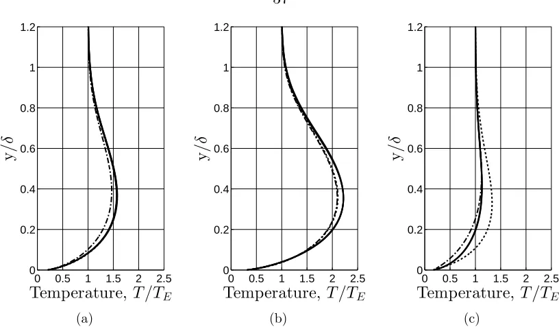
2.9 Example Temperature Profiles. . . 37

2.10 Evolution of Mass Fractions . . . 38

2.11 Evolution of Temperature . . . 40

2.12 u±a Profiles. . . 42

2.13 Overlay of the Computed Density, Cone, Shock, and Streamlines . . . 45

2.14 Zoomed-in Presentation of Density Contours in Nozzle. . . 45

2.15 Wall-Normal Distance from the Cone vs. the Radius in the Nozzle . . 46

2.16 Examples of Repeatability . . . 48

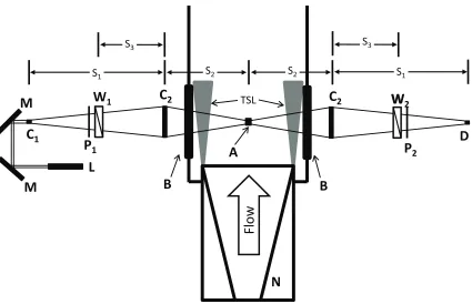
3.1 Annotated Schematic of the FLDI . . . 55

3.2 Boundary-Layer Thickness and Beam Profile. . . 59

3.3 Bench Test Schematic and Results: Sensitive Region . . . 61

3.4 Bench Test Schematic and Results: Equidistant Acoustic Wave . . . . 62

3.5 Density Eigenfunction and FLDI Probe Volume Sensitivity . . . 63

3.6 Averaged Density Eigenfunction and Response Function . . . 65

3.7 Sensitivity to Wavelength . . . 66

4.1 Sources of Wind-Tunnel Noise . . . 70

4.2 Tunnel Noise Time Traces . . . 72

4.3 Frequency Spectrum of Tunnel Noise Time Traces . . . 73

4.4 Wavelength Spectrum of Tunnel Noise Time Traces . . . 74

4.5 Spectrogram of Tunnel Noise . . . 75

4.6 Single Point FLDI Results Shot 2695 . . . 78

4.7 Single Point FLDI Results Shot 2702 . . . 79

4.8 Single Point FLDI Results Shot 2702 - Zoomed Time Trace . . . 80

(13)

4.10 Gas Opacity. . . 86

4.11 Windowed Spectra Shot 2711 . . . 87

4.12 Windowed Spectra Shot 2743 . . . 88

4.13 Narrowband vs. Broadband Disturbance . . . 88

4.14 Cross-Correlations, Shots 2711, 2743 . . . 89

4.15 Spectrograms of Shot 2711. . . 90

4.16 Spectrograms of Shot 2743. . . 91

4.17 Spectra For Shots 2711 and 2743 . . . 92

4.18 Traces and Cross-Correlations, Air, Low Enthalpy . . . 94

4.19 PSD Estimates, Air, Low Enthalpy . . . 96

4.20 Traces and Cross-Correlations, Air, High Enthalpy . . . 97

4.21 PSD Estimates, Air, High Enthalpy . . . 98

4.22 Schlieren Image of Instability in Air . . . 100

4.23 Traces and Cross-Correlations, N2, Low Enthalpy . . . 102

4.24 PSD Estimates, N2, Low Enthalpy . . . 103

4.25 Traces and Cross-Correlations, N2, Medium Enthalpy . . . 104

4.26 PSD Estimates, N2, Medium Enthalpy . . . 105

4.27 Traces and Cross-Correlations, N2, High Enthalpy . . . 106

4.28 PSD Estimates, N2, High Enthalpy . . . 106

4.29 Schlieren Image of Instability in N2 . . . 108

4.30 Traces and Cross-Correlations, CO2 . . . 109

4.31 PSD Estimates, CO2 . . . 110

5.1 Amplification Factor SNR . . . 114

5.2 Experimental Amplification Factor - All Shots . . . 115

5.3 Experimental Amplification Factor - Selected Shots . . . 117

5.4 Amplification Factor Calculation Methodology . . . 119

(14)

5.6 Computational-Experimental Comparison, N2 Low Enthalpy . . . 123

5.7 Computational-Experimental Comparison, CO2 . . . 124

5.8 Computational-Experimental Comparison, N2 High Enthalpy . . . 125

5.9 Computational-Experimental Comparison, Air High Enthalpy . . . 127

5.10 UE/(2δ) Scaling . . . 129

(15)

List of Tables

1.1 Characteristic Thermo-chemical Energies . . . 16

2.1 Uncertainty in Reservoir Conditions . . . 43

2.2 Uncertainty in Nozzle Conditions . . . 46

2.3 Uncertainty in Edge Conditions . . . 47

2.4 Shot Series Data from Hornung (1992) . . . 47

4.1 Run Conditions - Tunnel Noise . . . 72

4.2 RMS Tunnel Noise . . . 75

4.3 Run Conditions - Single Point FLDI . . . 80

4.4 Single Point Edge Conditions . . . 81

4.5 Double Point Edge Conditions - Dev. . . 86

4.6 Double Point Dev. Boundary Layer Instability Scaling . . . 93

4.7 Double Point Edge Conditions - Dev. . . 93

4.8 Double Point Air Boundary Layer Instability Scaling . . . 99

4.9 Double Point Edge Conditions - N2 . . . 101

4.10 Double Point N2 Boundary Layer Instability Scaling . . . 107

4.11 Double Point Edge Conditions - CO2 . . . 108

4.12 Double Point CO2 Boundary Layer Instability Scaling . . . 111

5.1 Amplification Factor Data Summary . . . 115

(16)

A.2 Tunnel Noise Reservoir Conditions . . . 158

A.3 Single Point Tunnel Run Parameters . . . 158

A.4 Single Point Reservoir Conditions . . . 158

A.5 Double Point Tunnel Run Parameters - Dev 1 Air . . . 159

A.6 Double Point Reservoir Conditions - Dev 1 Air . . . 159

A.7 Double Point Tunnel Run Parameters - Dev 1 CO2 . . . 159

A.8 Double Point Reservoir Conditions - Dev 1 CO2 . . . 160

A.9 Double Point Tunnel Run Parameters - Dev 2 Air . . . 160

A.10 Double Point Reservoir Conditions - Dev 2 Air . . . 160

A.11 Double Point Tunnel Run Parameters - Dev 2 CO2 . . . 161

A.12 Double Point Reservoir Conditions - Dev 2 CO2 . . . 161

A.13 Double Point Tunnel Run Parameters - Air . . . 162

A.14 Double Point Reservoir Conditions - Air . . . 162

A.15 Double Point Tunnel Run Parameters - N2 . . . 163

A.16 Double Point Reservoir Conditions - N2 . . . 163

A.17 Double Point Tunnel Run Parameters - CO2 - AR:100 . . . 164

A.18 Double Point Reservoir Conditions - CO2 - AR:100 . . . 164

A.19 Tunnel Noise Nozzle Exit Conditions . . . 165

A.20 Single Point Nozzle Exit Conditions . . . 165

A.21 Double Point Nozzle Exit Conditions - Dev 1 Air . . . 166

A.22 Double Point Nozzle Exit Conditions - Dev 1 CO2 . . . 166

A.23 Double Point Nozzle Exit Conditions - Dev 2 Air . . . 166

A.24 Double Point Nozzle Exit Conditions - Dev 2 CO2 . . . 167

A.25 Double Point Nozzle Exit Conditions - Air . . . 167

A.26 Double Point Nozzle Exit Conditions - N2 . . . 168

A.27 Double Point Nozzle Exit Conditions - CO2 . . . 168

(17)

A.29 Double Point Edge Conditions - Dev 1 Air . . . 169

A.30 Double Point Edge Conditions - Dev 1 CO2 . . . 170

A.31 Double Point Edge Conditions - Dev 2 Air . . . 170

A.32 Double Point Edge Conditions - Dev 2 CO2 . . . 171

A.33 Double Point Edge Conditions - Air . . . 171

A.34 Double Point Edge Conditions - N2 . . . 172

A.35 Double Point Edge Conditions - CO2 . . . 172

(18)

Chapter 1

Introduction

The study of boundary-layer transition (BLT) on hypersonic vehicles has been a

sub-ject of research for approximately a half century. Such continued support is indicative

of the intricate and potentially rewarding nature of the topic. Knowing the state of

the boundary layer is critical to the design of the vehicle.1 _{The surface heating rate}

and skin friction are several times higher when the boundary layer has transitioned

from laminar to turbulent. The primary design implications are that the thermal

pro-tection system must be more massive and the drag is increased when the boundary

layer is turbulent. The current state of the art is to design a vehicle conservatively

by sizing the thermal protection system over the entire vehicle to meet the

require-ments of turbulent boundary-layer heating rates. This is in large part due to the

lack of a reliable transition location prediction tool. The growth of the disturbances

in the boundary layer that precede transition is poorly understood, particularly at

conditions where gas dissociation and vibrational excitation must be considered. A

clearer understanding of the amplification process of disturbances in the boundary

layer in this flight regime would allow for a more intelligent sizing of thermal

protec-tion systems. In this work, the acoustic boundary-layer instability is characterized

with novel application of optical techniques in the previously unexplored regime where

1_{Reviews of the influence of BLT on high-speed vehicle design can be found in}_Schneider₍₂₀₀₄_),

(19)

thermo-chemical effects are important.

1.1

Design Implications of Boundary-Layer

Tran-sition

A case study of such design implications is the apparent weight and cost savings on

the National Aerospace Plane (NASP). The NASP was intended to be a single stage

to orbit vehicle, capable of transporting people by “tak[ing] off from Dulles Airport,

accelerat[ing] up to 25 times the speed of sound, attaining low Earth orbit or flying

to Tokyo within 2 hours”(Reagan, 1986).

The questions surrounding transition prediction were made apparent in a report

from the Defense Science Review Board on the NASP in 1988, “[t]he largest

un-certainty is the location of the point of transition from laminar to turbulent flow.

Estimates range from 20% to 80% along the body span. That degree of uncertainty

significantly affects the flow conditions at the engine inlet, aerodynamic heat transfer

to the structure and skin friction. These in turn affect estimates of engine

perfor-mance, structural heating and drag. The assumption made for the point of transition

can affect the design vehicle gross take off weight by a factor of two or more... In

view of the potential impact of uncertainties in the transition location, this is by

far the single area of greatest technical risk in the aerodynamics of the NASP

pro-gram” (DSB, 1988). Prior to the NASP program’s cancellation in 1993, the Defense

Science Review Board once again named boundary-layer transition as a critical area

of fundamental uncertainty, “[b]oundary layer transition and scramjet performance

cannot be validated in existing ground test facilities...”(DSB, 1992).

With certainty it can be said that BLT was a technical issue for the NASP and

(20)

billion USD from FY 1985-1993.2

1.2

Paths to Transition and the Dominant

Mech-anism

The path to transition in boundary layers is a subtle subject. Reshotko (2008) notes

that “[u]ntil about [1995], the predominant view of laminar-turbulent transition was

centered around the slow linear amplification of exponentially growing (“modal”)

dis-turbances..., preceded by a receptivity process to the disturbance environment and

followed by secondary instabilities, further nonlinearity, and finally a breakdown to

a recognizable turbulent flow.” Reshotko (2008) goes on to say that “[t]his picture

had to be urgently reconsidered in the early 1990s with the emergence of a literature

on transient growth,” which was motivated by the fact that “there are transition

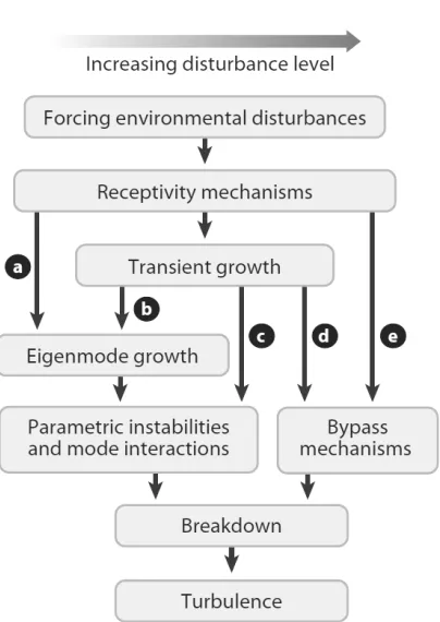
phenomena in flows that are linearly stable.” A flow-chart describing the paths to

turbulence was devised by Morkovin et al. (1994), where focus is placed on

under-standing the subtleties of this process (Fig. 1.1, taken from Fedorov (2011)). In

chapter 9 of Schmid and Henningson (2001) there is a thorough explanation of the

developments on this topic.

For a sharp, slender body in low-speed flight, at zero angle of attack, Tollmien

-Schlichting waves (“T-S waves”) are observed to be of large amplitude prior to

boundary-layer transition; these disturbances were experimentally characterized by

Schubauer and Skramstad (1948). This is in contrast to high-speed boundary layers

on the same vehicle geometry, where a key instability mechanism is the high-frequency

modes discovered byMack (1984). These modes are primarily acoustic in nature, are

always present if the boundary-layer edge Mach number is sufficiently large, and

2_{The funding figures can be found in}_Schwelkart₍₁₉₉₇_{), which references the NASP Joint Program}

(21)

Figure 1.1: Flow-chart describing the paths to turbulence was devised by

Morkovin et al.(1994), taken from Fedorov (2011) with permission.

can be the dominant instability mechanism when the wall temperature is sufficiently

low compared to the recovery temperature. “They belong to the family of trapped

acoustic waves. Owing to the presence of a region of supersonic mean flow relative

to the disturbance phase velocity, the boundary layer behaves as an acoustic

waveg-uide (schematically shown in [Fig. 1.2])” Fedorov (2011). Fedorov (2011) goes on to

provide a thorough explanation of “Path A” in Fig. 1.1 for the case of high-speed

boundary layers, supporting his conclusions of how the disturbances develop with

detailed stability calculations.

Mack termed the dominant higher frequency mode the “second mode,” although

Fedorov and Tumin (2011) suggest “that Mack’s definitions of modes are

inconsis-tent with conventional usage of the term normal modes.” However, most researchers

(22)

Figure 1.2: “Acoustic mode in a high-speed boundary layer, whereU(y) is the mean-flow profile, and p(y) is the pressure disturbance profile.” reproduced from Fedorov

(2011) with permission. The sonic line refers to where the local velocity (U(y)) equals the difference between the disturbance phase speed (c) and the local sound speed (a(y)). This is the location of the critical layer, where disturbance amplitudes are typically large Mack (1984), Fedorov(2011).

instability discovered by Mack, and this is the terminology usage in this thesis. The

larger growth rate of the acoustic instability relative to the “T-S waves” is seen in

Fig. 1.3(a). Additionally, it is seen that the second mode of largest growth rate is

two dimensional in nature. This second mode is the subject of study in this work.

In Fig. 1.3(b), a linear stability diagram is shown for an example case in T5. The

stream-wise imaginary wavenumber is shaded for values above 0, and more darkly

for larger values. Note the exceedingly high frequency of the acoustic mode, and the

narrowband at which it is most amplified. The most strongly amplified frequency is

observed to decrease with increasing distance from the tip of the cone; this frequency

is approximately equal to KUE/(2δ), where K is a constant of proportionality, UE

is the edge velocity, and δ is the boundary-layer thickness;3 _{this scaling is shown in} Fig. 1.3(b) as a thin white line. The constant of proportionality (K) for a certain

geometry is a function of (among other things) edge Mach number, because of the

im-plication on disturbance-phase velocity (Fig. 9.1 ofMack(1984)), and boundary-layer

temperature profile, because of the implication on disturbance wave number (Fig. 10.9

3_{In this work,}_δ_{refers to}_δ

99, where the local velocity in the boundary layer is 99% of the velocity

(23)

of Mack (1984)). The theoretical framework for the scaling of the most strongly

am-plified frequency can be found in Mack (1984, 1987); experimental support of this

scaling can be found inKendall (1975),Demetriades (1977) andStetson et al.(1983,

1984, 1989) (among many other reports). This scaling is extended to hypervelocity

conditions in this work.

(a)

Distance (mm)

F

re

q

u

en

cy

(k

H

z)

0 100 200 300 400 500 600 700 800 900 1000 0

500 1000 1500 2000 2500 3000

(b)

Figure 1.3: a: “Effect of Mach number of the maximum spatial amplification rate of the first and second mode waves... Insulated wall, wind-tunnel temperatures”

Mack (1984). At above Mach 4 the acoustic mode, which is two dimensional in nature, dominates the first mode. b: Example linear stability diagram computed from PSE-Chem for flow over a 5 degree half-angle cone, as in shot 2789 in T5. The stream-wise imaginary wavenumber is shaded for unstable values, and more darkly for more unstable values. The KUE/(2δ) scaling of the most amplified frequency is

shown as a thin white line, where K is a constant of proportionality that can range from 0.6-1.1.

1.3

Geometrical Acoustic Motivation

4

In this section the acoustic instability is examined with a geometrical acoustic

ap-proach. The propagation of acoustic waves within the boundary layer is profoundly

4

(24)

influenced by the velocity and sound speed gradients created by the action of viscosity

and heat conduction within the layer. These gradients form a waveguide that may

trap acoustic waves and provide a mechanism for the formation of large amplitude

disturbances. This suggests that geometrical acoustic analysis of these waveguides

can provide insights into the potential for boundary-layer acoustic instability. Here,

we outline the basics of geometric acoustics, apply the ray-tracing technique to

ex-ample problems, and then to high-speed boundary layers. The refractive behavior of

different high-speed boundary-layer profiles is compared.

The approach follows the classical ray-tracing approach to geometrical acoustics

in which the propagation of a wave-front is calculated by computing the paths (rays)

along which a point on the wave-front moves (Pierce,1989,Thompson,1972). From a

physical point of view, geometrical acoustics is a high-frequency approximation that

is valid when: 1) the wavelengths are small compared to the geometrical features

in the flow, in this case the thickness of the boundary layer; 2) the amplitude and

front curvature do not vary too rapidly along the wave-front; 3) cusps or folds

(caus-tics) do not form in the wave-front. In high-speed boundary-layer profiles, the most

amplified acoustic wavelength is known to be approximately 2 boundary-layer

thick-nesses (Mack,1984) and caustics are known to form (G. A. Kriegsmann and E. L. Reiss)

so we acknowledge from the outset that our results may be limited in quantitative

applicability and will be more qualitative in nature.

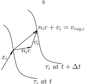
The rate of change of the position of a point xp on the wave-front can be written

as,

dxpi

dt =nic+vi =vray,i (1.1)

where vi is the local velocity, cis the local sound speed, and ni is the unit normal to

the wave-front τi (Fig.1.4). The speed of the wave-front normal to itself (c+nivi) is

in general different than the magnitude of the ray velocity |nic+vi|. The evolution of

(25)

x

i

n

i

c

v

i

n

i

c

+

v

i

=

v

ray,i

τ

i

at

t

τ

i

at

t

+

∆

t

Figure 1.4: Vector addition to find the velocity of the rays.

(1989) is used where the wave-front is described in terms of the wave-slowness vector

(si =▽τi),

dxi

dt = c2_s

i

Ω +vi, (1.2a)

dsi

dt =− Ω

c dc dxi

− 3

X

j=1 sj

dvj

dxi

, (1.2b)

where,

Ω = 1−visi, (1.3a)

si =

ni

c+nivi

. (1.3b)

1.3.1

Example Problems

Solutions to two example problems are presented here to provide basic insight into

geometric acoustics as well as to test our numerical methods. The first test problem

is an adaptation from the work ofGoodman and Duykers (1962). Analytic solutions

for ray paths are found for a quiescent gas with a parabolic sound speed profile of

the form c = c0 +α2y2, with 1/c2 = (1/c20)(1−y2/L2), and L =

p

(26)

example presented here,c0 = 340 m/s, α=

p

c0/10, and a rigid boundary at y= 0 is imposed. The solution for a ray path with initial angle of inclination to the horizontal

θ0, is

y/L= sinθ0sin (x/(Lcosθ0)). (1.4)

This solution (solid line) and results from numerically integrating Eqs. 1.2 (circular

markers) are shown to agree favorably in Fig. 1.5. In this scenario, sx is a constant,

per Eq. 1.2b. To calculate the point at which acoustic rays are refracted back to the

surface, it is recognized that the ray direction is parallel to the unit normal, n, when horizontal (Pierce, 1989), and from Eq 1.3b,

sx =

cosθ0 c0+ cosθ0vx0

=ch+vxh, (1.5)

where the subscript 0 indicates the local value at ray origin, and the subscript h indicates the local value where the ray is horizontal. Using this observation, the

wall-normal distance where the ray is refracted back to the surface can be obtained

algebraically. The predicted height (dashed line) shows favorable agreement with the

analytic and numerical results in Fig. 1.5. Note that the acoustic rays are refracted

towards a sound speed minimum, consistent with the vertical component of Eq.1.2b.

The second test problem is ray-tracing through the Sound Fixing and Ranging

(SOFAR) channel, as previously computed by Munk (1974), who assumed that the

sound speed in the ocean, c, varies as c=c(y) =c1(1 +ǫ(η(y) +e−η(y) −1)), due to temperature and density gradients, where c1 = 1.492 km/s, ǫ = 0.0074, η = η(y) = (z−z1)/(z1/2), and z1 = 1.3 km. Numerical integration of Eqs. 1.2 with this sound speed profile gives reasonable visual agreement with Munk’s results, although precise

quantitative comparison is not possible (Fig. 1.6). Acoustic rays are observed to be

(27)

1 1.5 2 0 0.2 0.4 0.6 0.8 1 c/c0 y / L

0

0.5

1

1.5

2

2.5

3

0

0.2

0.4

0.6

0.8

1

x/

(

π

L

cos(

θ

0

))

Figure 1.5: A slight modification to the problem posed by Goodman and Duykers

(1962), with the analytical solution (solid line), numerical integration (circular mark-ers), and predicted turning height (dashed line) showing good agreement. Initial angle of inclination of acoustic ray to the surface: θ0 = 30◦,60◦. The sound speed profile is plotted on the left.

1.48 1.5 1.52 1.54 0 1 2 3 4 c (km/s) D is ta n ce (k m )

0 10 20 30 40 50

0 1 2 3 4 -12 -8 -4 0 4 8 12 Distance (km)

Figure 1.6: Replication of the case done byMunk(1974), tracing acoustic rays through the SOFAR channel. The ordinate marks depth from the ocean surface, and the initial angle of the ray to the horizontal is denoted in degrees by a number overlaid on the line.

1.3.2

High-Speed Boundary Layers

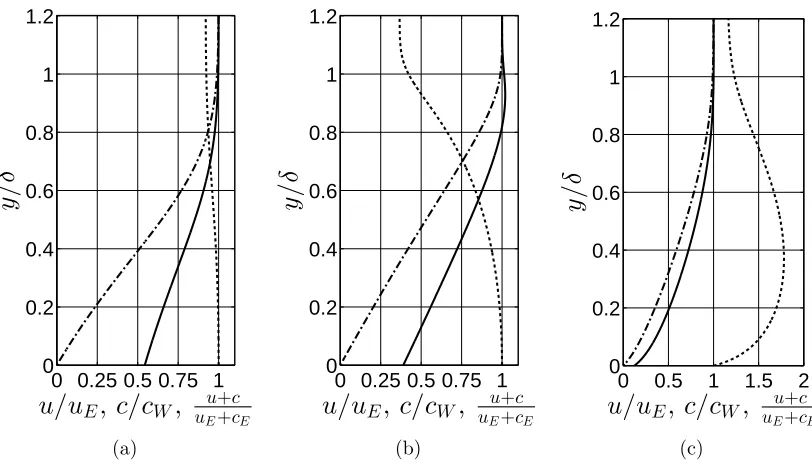
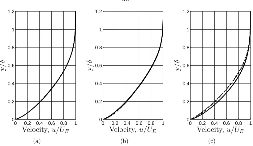
Geometric acoustic implications for a selection of high-speed boundary-layer profiles

are presented in this section. Boundary-layer profiles are computed using the

sim-ilarity solution for a laminar, compressible, perfect-gas flow on a flat plate (White,

2006). It was noted in the previous section that acoustic rays tend to be refracted

towards sound speed minima. The mean flow of the boundary layer modifies this and

(28)

to illustrate a range of u+cprofiles that are possible.

0 0.25 0.5 0.75 1 0

0.2 0.4 0.6 0.8 1 1.2

y

/

δ

u/u

E

,

c/c

W

,

_u_Eu+₊c_c_E

(a)

0 0.25 0.5 0.75 1 0

0.2 0.4 0.6 0.8 1 1.2

y

/

δ

u/u

E

,

c/c

W

,

_u_Eu+₊c_c_E

(b)

0 0.5 1 1.5 2

0 0.2 0.4 0.6 0.8 1 1.2

y

/

δ

u/u

E

,

c/c

W

,

_u_Eu+₊c_c_E

(c)

Figure 1.7: a: Boundary-layer profile forME = 1, γ = 7/5,TW =Tad. b:

Boundary-layer profile for ME = 6, γ = 7/5,TW =Tad. c: Boundary-layer profile for ME = 6,

γ = 7/5,TW =Tad/10. Each velocity profile (u/uE) is normalized by the edge value

(dash-dot). Each sound speed profile c/cW is normalized by the value at the wall

(dashed). Each combined profile (u+c)/(uE +cE) is normalized by the edge values

(solid).

Using Eq. 1.5, and assuming that the flow is locally parallel, the maximum angle

that is refracted back to the surface can be found. We postulate that the larger this

angle, the more unstable the boundary layer due to the larger amount of acoustic

energy trapped within the layer. The maximum angle of inclination is computed

for rays originating at the surface of the plate for a range of Mach numbers (ME =

0.25−8) with an adiabatic wall and three different ratios of specific heats in Fig.1.8(a).

The maximum angle increases with increasing Mach number, reaching a constant

value for ME ≥ 5. Wall temperature ratio (TW/Tad, where Tad is the adiabatic wall

temperature) is another important parameter in determining the maximum initial

angle of inclination for rays originating at the surface of the plate (Fig. 1.8(b)); at

(29)

wall normal distance of the origin of the acoustic ray is varied for an adiabatic plate

withME = 6. Fewer rays are trapped as the ray origin is translated from the surface.

The results in Figs. 1.8(a),1.8(b), and1.8(c)do not change with Rex, where xis the

distance from the leading edge, because the flow field is assumed to be locally parallel

and the boundary-layer profiles are self-similar.

The non-parallel nature of the flow field can be included by interpolating the

velocity and sound speed profiles calculated from the similarity solution for a certain

range of Rex and solving Eqs.1.2. In Fig.1.9, ray traces originating from the surface

of an adiabatic flat plate withME = 1 andγ = 7/5 with an initial angle of inclination

of θ0 = 56◦,57◦,58◦ are observed to bracket the value predicted in Fig. 1.8(a). The edge Mach number is increased to 6 for the rays in Fig. 1.10 and ray traces with an

initial angle of inclination of θ0 = 67◦,68◦,69◦ bracket the maximum value predicted in Fig. 1.8(a). Changing the boundary condition at the wall to TW =Tad/10 should

increase the maximum initial angle of inclination per Fig.1.8(b). This is reflected in

(30)

0 1 2 3 4 5 6 7 8 30 35 40 45 50 55 60 65 70 75 80

γ= 6/5

γ= 7/5

γ= 5/3

Edge Mach Number: ME

In cl in a ti o n to p la te : θ0 (a)

10−2 10−1 100 101

30 35 40 45 50 55 60 65 70 75 80 85 90

Wall Temperature Ratio: TW/Tad

In cl in a ti o n to p la te : θ0

γ = 6/5

γ = 7/5

γ = 5/3

(b)

0 0.25 0.5 0.75 1

0 10 20 30 40 50 60 70 80 γ=6/5 γ=5/3 γ=7/5

Distance from wall: y/δ

In cl in a ti o n to p la te : θ0 (c)

Figure 1.8: a: Largest angle of inclination to the plate of acoustic ray that is refracted back to the surface, ME = 0.25−8,γ = 6/5,7/5,5/3,TW =Tad. b: Largest angle of

inclination to the plate of acoustic ray that is refracted back to the surface, ME = 6,

γ = 6/5,7/5,5/3, TW = KTad, where K is varied between 10−2 and 5. c: Largest

angle of inclination to the plate of acoustic ray that is refracted back to the surface at different wall normal origins, ME = 6, γ = 6/5,7/5,5/3,TW =Tad.

300 320 340 360 380 400 420 440

0 2 4 6 8

δ

99 x (mm) y (m m )

(31)

50 60 70 80 90 100 110 120 130 140 150 160 0

1 2 3 4 5

6

δ

99

x (mm)

y

(m

m

)

Figure 1.10: Ray traces for ME = 6, γ = 7/5, TW = Tad, with θ0 = 67◦,68◦,69◦ at Rex0 = 1×105.

50 55 60 65 70 75 80

0 0.5 1 1.5 2

δ

99

x (mm)

y

(m

m

)

(32)

1.3.3

Summary

Ray-tracing in high-speed boundary layers has been used to explore the potential for

acoustic energy trapping as function of edge Mach number, wall temperature ratio,

and thermodynamic parameters. We proposed a figure of merit for acoustic energy

trapping as the critical angle of inclination for rays originating in the boundary that

are trapped, i.e., these rays always stay within the boundary layer. Using this concept,

we find that an increasing amount of acoustic energy is trapped with increasing edge

Mach number (ME), and decreasing wall temperature ratio (TW/Tad). These trends

agree qualitatively with the results of high-speed boundary-layer stability calculation

by Mack (1984).

1.4

Motivation For Hypervelocity Instability Study

“High-enthalpy” or “hypervelocity” fluid-mechanics research is the study of

high-speed flow fields “that are both hypersonic and high velocity, rather than merely

hypersonic” (Stalker, 1989). The term “hypersonic” generally refers to flows with a

characteristic Mach number of greater than five, but the term “high velocity” is more

relative. Following Hornung (1993), we estimate the ordered-kinetic energy of the

free-stream gas flowing over a vehicle moving at U∞ as U∞2/2; so, a vehicle moving at 3 km/s or 6 km/s results in ordered kinetic energies of 4.5 MJ/kg or 18 MJ/kg,

respectively. These large ordered kinetic energies can be of the same order as the

characteristic thermo-chemical energy scales in a flow-field of interest; for example,

the characteristic energies of dissociation (D) and vibrational excitation (Eν) for N2,

O2, and CO2 are listed in Table 1.1.5 When the free-stream ordered kinetic energy

is a significant fraction of the characteristic energy of dissociation or vibration, these

5_{The tabulated thermo-chemical data is adapted from}_McQuarrie₍₂₀₀₀_{). For CO}

2, the reaction

CO2 → CO + 1₂O2, and the lowest energy doubly degenerate mode of vibrational excitation are

(33)

effects can be present in the flow-field.

Table 1.1: Characteristic thermo-chemical energies

DN2 DO2 DCO2 EνN2 EνO2 EνCO2 33.6 MJ/kg 15.4 MJ/kg 6.3 MJ/kg 1000 kJ/kg 590 kJ/kg 180 kJ/kg

For blunt-body flows, dissociation of the free-stream gas can occur, which can

result in lower temperature and higher density than if the gas were thermo-chemically

frozen. This can change the shockwave shape and stand-off distance over a vehicle,

which can change the surface pressure distribution and heat-flux.

An essential aspect of studying hypersonic slender-body boundary-layer instability

at high enthalpy is characterizing the energy exchange between the thermo-chemical

and fluid-mechanical processes. These effects are termed “high-enthalpy effects” on

boundary layers. Thermo-chemical processes are only relevant at high-enthalpy

con-ditions where the ordered kinetic energy of the flow is high enough so that chemical

reactions and relaxation processes occur. If the energy is high enough, and if the

fluid-mechanical and thermo-chemical processes proceed at comparable time scales,

then energy exchange may occur.

Of particular interest is the exchange of energy between the high-frequency

acous-tic instability in a hypersonic boundary layer and molecular vibrational relaxation

processes. For certain conditions, the time scale of the instability which goes as the

edge velocity on twice the boundary-layer thickness (f ≈ UE/(2δ)) is of the order

1 MHz. Vibrational relaxation processes can be of this time scale at conditions in a

hypersonic boundary layer, so energy exchange may occur, and the instability could

be damped.

1.4.1

Energy Exchange and pdV Work

In a non-equilibrium gas, the sound speed is not unique because the thermodynamic

(34)

s(p, ρ, q), where q is a non-equilibrium variable (Vincenti and Kruger, 1965). The frozen sound speed (a2

f = (∂p/∂ρ)s,q) is evaluated with q fixed, and the equilibrium

sound speed (a2

e = (∂p/∂ρ)s,q∗) is evaluated with the non-equilibrium variableq =q∗

at its value if the gas were in local equilibrium. The ratio of frozen sound speed

to equilibrium sound speed (af/ae) is a measure of the capacity of a gas to absorb

acoustic energy.

Following section 4 of chapter 8 inVincenti and Kruger(1965), a model of a piston

harmonically oscillating in a constant area duct occupied by a non-equilibrium gas

can be used as an example of how acoustic waves may be damped by an exchange of

energy with the gas. An indication of the absorption of acoustic energy can be shown

on a P-v diagram. P-v cycles of an acoustic wave oscillating at angular frequency ω with the time scale of relaxation τ show that an ellipse of finite width is traced when the pressure and density of the gas are out of phase (Fig. 1.12(a)). If the

sound-speed ratio (af/ae) is fixed at a number that is larger than unity, and the time

scale matching is varied, the ellipse thickness varies with the time scale (ωτ), and is

thickest when the scale is of order 1. The ellipse thickness indicates the possibility

of pdV work, which may be interpreted as an exchange of energy from the acoustic wave to the internal energy of the gas; the broader the ellipse, the greater the energy

exchange. Qualitatively, two requirements for energy exchange are evident: 1) the

time scales of relaxation and acoustic wave oscillation must be similar, and 2) the gas

must have sufficient internal vibrational or rotational energy so that energy exchange

(35)

−1 −0.75 −0.5 −0.25 0 0.25 0.5 0.75 1 −1 −0.75 −0.5 −0.25 0 0.25 0.5 0.75 1

Specifi_{c Volume (%)}

P re ss u re (% )

(af/ae)2= 1.00,ωτ= 1.0

(af/ae)2= 1.09,ωτ= 1.0

(a)

−1 −0.75 −0.5 −0.25 0 0.25 0.5 0.75 1 −1 −0.75 −0.5 −0.25 0 0.25 0.5 0.75 1

Specifi_{c Volume (%)}

P re ss u re (% )

(af/ae)2= 1.09,ωτ ≈0

(af/ae)2= 1.09,ωτ = 1.0

(af/ae)2= 1.09,ωτ ≈∞

(b)

Figure 1.12: a: P-v cycles of an acoustic wave with a time scale match (ωτ = 1), with different ratios of sound speed (af/ae) b: for a fixed sound-speed ratio (af/ae), P-v

cycles for disparate time-scale ratios (ω/τ). This illustrates the two requirements for pdV energy exchange: 1) the time scales of relaxation and acoustic wave oscillation must be similar, and 2) the gas must have sufficient internal energy so that energy exchange is possible.

1.4.2

Simple Acoustic-Wave Attenuation Model

A simple acoustic-wave attenuation model is introduced in this subsection. Following

the development inPierce(1989) andThompson(1972), the absorption coefficientαa

for a gas where there is a small contribution to the heat capacity from the vibrational

degree of freedom (cv,i ≪cp)can be written as,

αa=αc+ X

i

αr,i, (1.6a)

αc =

µω2 2ρLa3f

4 3+

γf −1

Pr

, (1.6b)

αr,i =

π(γf −1)cv,i

λcp

ωτi

1 + (ωτi)2

. (1.6c)

Here, αc is the classic absorption coefficient due to viscous and thermal attenuation,

µ is the viscosity, ρL is the mean local density, af is the frozen sound speed, γf

is the frozen ratio of specific heats, and Pr is the Prandtl number. Additionally,

(36)

are the wavelength and angular frequency of the acoustic wave, respectively; cv,i is

the constant-volume specific heat contribution from a relaxation process i (e.g. the vibrational mode of N2), and cp is the equilibrium constant-pressure specific heat.

The classic absorption coefficient result is from Stokes and Kirchhoff, so it is

termed SK attenuation (Thompson, 1972). Also inThompson (1972), the SK

atten-uation results are supported by summarized experimental data up to a time scale

where the collision rate becomes comparable; the scale µω/P = 0.1 is suggested, where µ is the local viscosity, ω is the angular frequency of the disturbance, and P is the local pressure. This implies that the SK attenuation coefficient can be used to

≈5 MHz for conditions in a typical boundary layer during a T5 test.

10−2 10−1 100 101 102 10−2

10−1 100

ωτi

λ

αr,

i

/

(

λ

αr,

i

)m

a

x

(a)

101−1 100 101

1.02 1.04 1.06 1.08 1.1

T /Θ_v

(

af

/a

e

)

2

(b)

Figure 1.13: a: The absorption coefficient for a single relaxation process normalized by its maximum value illustrating the time scale dependence. b: The ratio of frozen to equilibrium sound speed as a function of the ratio of the temperature (T) to characteristic vibrational temperature (Θv) for a linear polyatomic molecule with a

single non-degenerate relaxing vibrational degree of freedom.

From Eq. 1.6c it is clear that the absorption coefficient due to a relaxation

pro-cess is highly time scale dependent, this is highlighted in Fig. 1.13(a). Additionally,

the frozen to equilibrium sound-speed ratio (af/ae) is an indicator of the magnitude

of (λαr,i)max. For a chemically frozen gas, this is a function of the extent to which

(37)

lin-ear polyatomic molecule with a single non-degenerate relaxing vibrational degree of

freedom is highlighted in Fig. 1.13(b).

The absorption coefficient for CO2 is of particular interest because there is a

doubly-degenerate vibrational mode at moderate characteristic temperature, Θv =

960 K; this is relatively low compared with the characteristic temperatures of

vibra-tion for N2 and O2, which are 3374 K and 2260 K, respectively. The implication is

that CO2 has a relatively high capacity to attenuate high-frequency waves, possibly

even those in the boundary layer of a high-speed vehicle. The assumption that the

contribution to the specific heat capacity from the vibrational degree of freedom is

small (cv,i ≪cp) is not valid in the temperature ranges discussed here. For this

rea-son, the wavenumber is found from the dispersion relation for a relaxing gas given as

Eq. 10-8.7 in Pierce (1989), and the imaginary portion is reported as the absorption

coefficient.

An example absorption coefficient curve (Fig.1.14(a)) highlights the relative

spec-trum of attenuation due to SK dissipation and vibrational relaxation for CO2 at

P = 25 kPa, T = 1500 K. These results show attenuation of≈5-30% per wavelength over a large frequency band. This is a large value for the absorption coefficient when

compared with that of N2 for the same conditions (Fig. 1.14(b)).

In these calculations, the relaxation rates for CO2 and N2 are taken fromCamac

(1966) and Millikan and White (1963), respectively. In Camac (1966), it is observed

that all four vibration modes relax at the same rate, and the data are summarized

along with eight other references where vibrational relaxation data were reported

at lower temperatures. Gaydon and Hurle (1963) caution that “[t]he relaxation of

carbon dioxide is very sensitive to the presence of impurities,” which can effectively

reduce the relaxation time. The thermodynamic data were calculated using

statisti-cal mechanics, as in McQuarrie (2000). The thermodynamic properties are checked

(38)

104 105 106 10−2

10−1 100

Frequency (Hz)

λ

α

Vibration Thermal-Viscous Sum

(a)

104 105 106

10−3 10−2 10−1 100

Frequency (Hz)

λ

α

(b)

Figure 1.14: a: Absorption coefficient for CO2 atP = 25 kPa,T = 1500 K. The solid line represents the total absorption coefficient, which is the sum of the viscous-thermal term (dotted line), and the term due to the vibrational relaxation (dash-dot line). b: Absorption coefficient for N2 (dotted line) and CO2 (solid line) at P = 25 kPa, T = 1500 K.

in McBride et al. (2002) using Cantera (Goodwin, 2003). The viscosity is evaluated

from curve fits as in Blottner et al. (1971).

1.5

Hypervelocity Transition in T5

Boundary-layer stability and transition in high-enthalpy facilities has been studied

extensively for 20 years in the T5 hypervelocity shock tunnel. Germain (1993) and

Germain and Hornung(1997) conducted a series of transition experiments on a sharp

5 degree half-angle cone at zero angle of attack in the T5 hypervelocity shock

tun-nel. Transition Reynolds number was measured for a range of free-stream

condi-tions and gasses. The transition Reynolds number was determined by noting the

location of departure of laminar heating rates. The surface heating rates were

mea-sured by heat-transfer gauges constructed of type E thermocouples (manufactured by

Medtherm Corporation) that were mounted flush to the surface. Germainfound that

the transition Reynolds number increases with increasing reservoir enthalpy, when

(39)

with lower dissociation and vibrational energies. Additionally, resonantly enhanced

shadowgraphy was used to characterize the flow structures. Based on these results,

Germain and Hornung proposed that the dominant instability mechanism was the

Tollmien-Schlichting mode in those experiments.

Transition and stability work on a sharp 5 degree half-angle cone in T5 continued

in the 1990’s, as reported in Adam (1997) and Adam and Hornung (1997). They

too note that transition Reynolds number increases as the reservoir enthalpy is

in-creased, and this effect is more pronounced in CO2 than in air. Adam then used the

tabulated transition Reynolds numbers based on reference temperature and found

the results to be “within striking distance” of Re-entry F free-flight data reported in

Wright and Zoby(1977). Adam also used BLIMPK6 _{to compute the similar}

non-equilibrium boundary-layer profiles on the cone to understand the extent to which the

frictional heating affected the thermo-chemical properties of the boundary layer, i.e.,

quantifying the dissociation level of different gases at different condition as a function

of distance along the cone surface.

Boundary-layer stability control research then followed in T5, as reported in

Rasheed(2001) andRasheed et al.(2002). In that work, researchers used a novel

pas-sive scheme to damp the acoustic instability in a hypervelocity boundary layer on a

five degree half-angle cone. Half of the surface of the test article was allocated to serve

as a smooth control, and the opposing half was an ultrasonically absorptive surface.

The transition Reynolds number on the smooth surface was consistent with previous

work, while the half with the ultrasonic absorptive surface exhibited significant

in-creases in transition Reynolds number. Because the passive boundary-layer instability

control scheme was aimed at damping the acoustic instability, and the scheme proved

effective in increasing the transition Reynolds number, one might conclude that the

most unstable mode is acoustic in nature, not the viscous or Tollmien-Schlichting

6_{BLIMPK stands for Boundary Layer Integral Matrix Procedure with Kinetics, and more}

(40)

mode as suggested inGermain (1993) and Germain and Hornung(1997).

Fujii(2001) andFujii and Hornung(2003) investigated attachment line

boundary-layer transition on a swept cylinder in T5. Most relevant to the present work were

the efforts made to quantify the role of energy exchange between the boundary-layer

instability and the fluid, which is described in detail in Fujii and Hornung (2001).

They proposed that if the time scale of a relaxation process in gas is nearly matched

to the time scale of the acoustic instability in the boundary layer, significant energy

may be scrubbed from the instability. This removal of energy from the boundary-layer

instability would ultimately manifest itself as an increase in boundary-layer transition

Reynolds number. Quantitative results for absorption were computed from a model

of high-frequency sound waves propagating through a relaxing gas.

Further boundary-layer instability control research has continued in T5, as

re-ported inLeyva et al.(2009a,b) andJewell et al.(2011,2012,2013). In this research,

the ultimate goal is to increase the transition Reynolds number in a test gas by

intro-ducing a different gas with lower dissociation and vibrational energies than the test

gas. By introducing a gas into the boundary layer that has thermo-chemical

prop-erties which may attenuate acoustic waves, the researchers suggest that the acoustic

instability will be damped, and the transition Reynolds number will be increased.

1.6

Project Scope and Outline

The disturbances preceding boundary-layer transition on a slender body at

hyperve-locity flight conditions are characterized in this work. A sharp five-degree half-angle

cone at zero angle of attack is used as the test article because of the canonical nature

of the geometry. Ground testing was performed in the T5 hypervelocity free-piston

driven reflected-shock tunnel to enable the study of thermo-chemical/fluid-dynamic

(41)

In chapter 2, operation of the T5 facility is described; the test procedure and

calculation of run conditions are presented with examples and estimates of error. In

chapter 3, the focused laser differential interferometry technique (FLDI) is used to

measure the hypervelocity boundary-layer disturbances and is characterized. In

chap-ter 4, results from the application of the FLDI technique to T5 flows are presented;

tunnel noise and boundary-layer disturbance spectra are highlighted. The results of

experiments where narrowband boundary-layer disturbances were observed at two

(42)

Chapter 2

Facility and Run Conditions

The test facility and method of calculating the run conditions are described in this

chapter. The test procedure is described in detail, noting alterations to past efforts.

The run conditions are calculated in three stages, the reservoir, the nozzle, and then

the mean flow over the cone. The propagation of error in these calculations is

esti-mated. Comments are made on the repeatability of T5 tunnel operation. Example

profiles are provided throughout this chapter for context.

2.1

Facility and Test Procedure

All measurements are made in T5, the free-piston driven reflected-shock tunnel at the

California Institute of Technology (Fig. 2.1). It is the fifth in a series of shock tunnels

designed to simulate high-enthalpy real gas effects on aerodynamics of vehicles flying

at hypervelocity speeds through the atmosphere. More information regarding the

capabilities of T5 can be found in Hornung (1992).

An experiment is conducted as follows: a 120 kg aluminum piston is loaded into

the compression tube/secondary reservoir junction. A secondary diaphragm (mylar,

127µm thick) is inserted at the nozzle throat at the end of the shock tube near the test section and a primary diaphragm (stainless steel, 7-10 mm thick) is inserted at the

(43)

Figure 2.1: A schematic of T5 with a blown up view of each of the major sections.

tube are evacuated. The shock tube is filled with the test gas (in the present study,

air, CO2, or N2 to 20-150 kPa), the compression tube is filled with a He/Ar mixture

to≈45-150 kPa and the secondary reservoir is filled with air to≈2-11 MPa. The air

in the secondary reservoir is released, driving the piston into the compression tube.

This piston motion adiabatically compresses the driver gas of the shock tunnel to the

rupture pressure of the primary diaphragm (≈ 20-120 MPa). Following the primary

diaphragm rupture, a shock wave propagates in the shock tube, is reflected off the

end wall, breaking the secondary diaphragm and re-processing the test gas. The test

gas is then at high temperature (≈ 2000-9000 K) and pressure (≈ 15-80 MPa) with

negligible velocity, and is then expanded through a converging-diverging contoured

nozzle to ≈ Mach 5.5 in the test section.

Throughout the testing campaign for this work, it became apparent that there

was opportunity to improve the quality of the flow over the model. Improvement was

made by using higher quality gas to fill the shock tube and by cleaning the shock

tube more thoroughly between experiments. The quality of the gas used to fill the

shock tube, and the shock tube cleaning procedure were fixed after shot 2760 because

(44)

procedure was concurrent with the conclusion of the development phase of the project.

A more thorough explanation and examples of inconsistent and consistent

instability-measurement results are found in section 4.3.1.

2.2

Reservoir Conditions Calculation

Initial shock tube pressureP1, measured primary shock speedUS, and reservoir

pres-sure PR, are used to compute the reservoir conditions for each shot. The primary

shock speed and initial shock tube pressure are used to calculate the thermodynamic

state of the gas after being processed by the primary and reflected-shock waves,

assuming thermo-chemical equilibrium. The gas pressure behind the reflected-shock

wave is changed isentropically, assuming chemical-thermodynamic equilibrium, to the

measured reservoir pressure to account for the weak expansion or compression waves

that are reflected between the contact surface and the shock tube end.

Thermo-chemical calculations are performed using Cantera (Goodwin, 2003) with the Shock

and Detonation Toolbox (Browne et al.,2006). The appropriate thermodynamic data

are found in the literature (Gordon and McBride, 1999, McBride et al., 2002). The

reservoir conditions for each experiment are tabulated in section A.1.

An example from shot 2789 shows the reservoir pressure time traces from the north

and south gauges1 _{in Fig} _2.2(a)_{. The mean between the gauges of the time-average}

during the steady pressure period is shown in the text box along with the standard

deviation which serves as an estimate of error in the measurement.

An X-t diagram for shot 2789 is shown as Fig.2.2(b). The pressure traces of the four stations in the shock tube and the reservoir are plotted at their spatial locations.

The shock speed is calculated by dividing the transit distance by the transit time. The

shock speed between station 4 and the reservoir transducer is not reported because

1

(45)

the reservoir pressure tap is not designed for accurate time of arrival measurements.

The shock speed between stations 3 and 4 is used for the thermo-chemical equilibrium

calculations because it is estimated by X-tdiagram that this location corresponds to the steady portion of the test gas slug (B´elanger, 1993).

0 0.5 1 1.5 2 2.5

0 10 20 30 40 50 60 70 ¯

PR= 56.4±1.8 MPa

Time (ms) R es er vo ir P re ss u re , PR (M P a ) (a) 0 2 4 6 8 10 12 −3 −2.5 −2 −1.5 −1 −0.5 0 0.5 S T E n d W a ll

US=4.19 km/s

US=3.85 km/s

US=3.49 km/s

PST1 PST2 PST3 PST4 PR

Distance from End Wall(m)

T im e (m s) (b)

Figure 2.2: Left: Example reservoir pressure trace from shot 2789. In the reservoir pressure trace, the north gauge’s trace is black; the south gauge’s trace is gray. Right: X-t diagram showing the propagation of the incident shock of speed US, as well as

pressure traces at 5 stations along the shock tube from shot 2789.

2.3

Nozzle Calculation

The steady expansion through the contoured nozzle (outline in Fig. 2.3) from the

reservoir to the free-stream is modeled by the axisymmetric, reacting Navier-Stokes

equations as described in by Candler (2005), Johnson (2000), and Wagnild (2012).

The translational and rotational degrees of freedom are assumed to be in equilibrium.

The vibrational degree of freedom is allowed to deviate with equilibrium with the

translational/rotational modes. The boundary layer on the nozzle wall is assumed to

be turbulent and modeled by one equation as in Spalart and Allmaras (1992) with

the Catrisa and Aupoix (2000) compressibility correction. The grid is generated by

(46)

−100 0 100 200 300 400 500 600 700 800 900 0

50 100 150

r

(m

m

)

x (mm)

Figure 2.3: An outline of the T5 contoured nozzle of area ratio 100.

2.3.1

Nozzle Freezing Examples

The term nozzle freezing is used to indicate when a chemical-thermodynamic

reac-tion rate is not high enough to match the characteristic time scale in the nozzle.

Typically, reaction rates are a strong function of temperature, and reactions cease if

the temperature drops too rapidly, hence the term freezing. This is a known issue

in ground-testing because the gas at the exit of the nozzle can be partially

disso-ciated and vibrationally excited relative to the desired free-stream condition that

corresponds to a free-flight condition. This issue and others pertaining to high-speed

ground-testing are discussed in broader context inStalker(1989) andHornung(1993).

The aim of the subsequent discussion is to give quantitative examples of the

freez-ing effect by showfreez-ing the computed evolution of the translational/rotational

temper-ature (Tt/r), the vibrational temperature (Tv),2 and the chemical composition along

the centerline in the nozzle when the test gas is air, CO2, and N2 at nominally

sim-ilar reservoir conditions (reservoir enthalpy hR ≈9 MJ/kg, and reservoir pressure

PR ≈17 MPa)3.

For air as the test gas, the translation/rotational and vibrational temperatures

do not have a discernible difference from each other, but are elevated relative to a

free-flight condition (Fig. 2.4(a)). NO and O are frozen downstream of the location

2

The vibrational temperature (Tv), is a figure that defines the quantity of energy that excites

the vibrational degree of freedom. This is not to be confused with the characteristic temperature of vibration, Θv = hν/kb, whereh is Planck’s constant, kb is Boltzmann’s constant, and ν is the

frequency of the oscillator.

3

(47)

A/A∗_{=10, reducing the amount of O}

2 and N2 present at the nozzle exit (Fig.2.4(b)),

where A/A∗ _{is the area ratio with respect to the area at the nozzle throat,} _A∗_.

100 101 102

0 0.2 0.4 0.6 0.8 1

Area Ratio

T

/

TR

Tt/r, Tv

(a)

100 101 102

10−2 10−1 100

Area Ratio

M

a

ss

F

ra

ct

io

n

N2

O2

NO

O

(b)

Figure 2.4: Air shot (2767). Labels are placed at the nozzle exit (area ratio 100), the other end of each line segment represents the value at the reservoir (area ra-tio 9). The area rara-tio of 1 denotes the converging-diverging nozzle throat. Left: Translation/rotational temperature Tt/r and vibrational temperature Tv for air. The

subscript R denotes the value at the reservoir. Right: Species recombination in the nozzle for air.

To assess the effect of the dissociation products of air being frozen in the flow,

the difference in free-stream enthalpy and velocity is chosen to differentiate between

the gas in its computed thermo-chemical non-equilibrium state (Fig. 2.4(b)) with a

comparable equilibrium state. Cantera is used to compute the equilibrium

thermo-chemical state of the gas at the same free-stream temperature and pressure. At that

temperature and pressure, the air is nearly totally recombined (yN O <0.02%)4, and

the free-stream enthalpy is 625 kJ/kg lower (≈ 7% of the reservoir enthalpy, hR),

resulting in an increase in velocity of 160 m/s (4%).

With CO2 as the test gas, the translation/rotational and vibrational temperatures

also do not have a discernible difference from each other, but are elevated relative to

a free-flight condition (Fig. 2.5(a)). CO and O2 concentrations are chemically frozen

downstream of the locationA/A∗_{=10 at levels substantially higher than equilibrium}

4_y

(48)

at the nozzle exit, reducing the amount of CO2 in the test gas(Fig. 2.5(b)). The

energy required to dissociate CO2 is lower than for O2 and N2 (quantitative values

of relative dissociation levels can be found for all conditions in section A.1). Because

it does not have correspondingly higher recombination rates, CO2 experiments tend

to have more free-stream dissociation than air or N2 experiments at similar reservoir

conditions. Comparing CO2 experiments relative to air experiments for similar

reser-voir conditions, the gas at the nozzle exit is of lower velocity and lower Mach number

because it is hotter and more dissociated.

100 101 102

0 0.2 0.4 0.6 0.8 1

Area Ratio

T

/

TR

Tt/r, Tv

(a)

100 101 102

10−2 10−1 100

Area Ratio

M

a

ss

F

ra

ct

io

n

CO2

O2

CO

(b)

Figure 2.5: CO2 shot (2791). Labels are placed at the nozzle exit (area ratio 100), the other end of each line segment represents the value at the reservoir (area ratio 9). The area ratio of 1 denotes the converging-diverging nozzle throat. Left: Trans-lation/rotational temperature Tt/r and vibrational temperature Tv for CO2. The subscript R denotes the value at the reservoir. Right: Species recombination in the nozzle for air. The unlabeled line in (b) is the species O.

Dissociation products of CO2 being frozen in the flow also cause a difference in

free-stream enthalpy and velocity between the gas in its computed thermo-chemical

non-equilibrium state (Fig. 2.5(b)) and a corresponding equilibrium state. At the

same free-stream temperature and pressure, but in thermo-chemical equilibrium, the

CO2 is nearly totally recombined (99.8%), and the free-stream enthalpy is 2.4 MJ/kg

lower (≈ 27% of hR), resulting in an increase in velocity of 700 m/s (22.5%). This

(49)

than for air or N2 shots.

With N2 as the test gas, the translation/rotational and vibrational temperatures

do have a discernible difference from each other, and are elevated relative to an

equilibrium condition at the nozzle exit (Fig. 2.6(a)). N2 has a higher dissociation

energy relative to air and CO2, and is high relative to the reservoir enthalpy in this

example, so there is almost no N at the nozzle exit (Fig. 2.6(b)). Comparing N2

shots to air shots, the gas at the nozzle exit is colder, less dissociated, and has higher

velocity and higher Mach number.

100 101 102

0 0.2 0.4 0.6 0.8 1

Area Ratio

T

/

TR

Tv

Tt/r

(a)

100 101 102

10−2 10−1 100

Area Ratio

M

a

ss

F

ra

ct

io

n

N2

(b)

Figure 2.6: N2 shot (2773). Labels are placed at the nozzle exit (area ratio 100), the other end of each line segment represents the value at the reservoir (area ra-tio 9). The area rara-tio of 1 denotes the converging-diverging nozzle throat. Left: Translation/rotational temperature Tt/r and vibrational temperatureTv for N2. The subscript R denotes the value at the reservoir. Right: Species recombination in the nozzle for air. Labels are placed at the nozzle exit, the other end of each line segment represents the value at the reservoir. The unlabeled line in (b) is the species N.

An estimate of the loss in free-stream velocity for shot 2773 due to the

freez-ing of the N2 in a partially vibrationally excited state can be estimated by

follow-ing Vincenti and Kruger(1965). Neglecting contributions from electronic effects, the

mass-specific internal energy can be written as

e=RT2∂lnQ ∂T =RT

2

t/r

∂lnQt

∂Tt/r

+RT_t/r2 ∂lnQr ∂Tt/r

+RT_v2∂lnQv ∂Tv

(50)

whereQis the partition function, which for the translational (subscript t), rotational (subscript r), and vibrational (subscript (v) degrees of freedom are

Qt=

2πmkTt/r

h2

3/2

V, (2.2a)

Qr =Tt/r/Θr, (2.2b)

Qv =

1

1−exp(−Θv/Tv)

, (2.2c)

where Tt/r is the translational/rotational temperature, Tv is the vibrational

temper-ature, m is the mass of N2, k is Boltzmann’s constant, and h is Planck’s constant. This results in the internal energy

e= 3

2RTt/r+RTt/r+

Θv/Tv

exp(Θv/Tv)−1

RTv. (2.3)

For shot 2773, Tt/r = 804 K so the contribution to the internal energy is 597 kJ/kg,

and Tv = 3163 K so the contribution is 525 kJ/kg. If we assume that the vibrational

temperature were to relax to the translational temperature, Tv = 804 K, the

contri-bution to the internal energy would be 15 kJ/kg. To assess what effect this has on

the free-stream velocity the free-stream mass-specific enthalpy,h=e+p/ρ, is written as

h= 7

2RTt/r+

Θv/Tv

exp(Θv/Tv)−1

RTv. (2.4)

The free-stream enthalpies of the gas when vibrationally excited and in

thermody-namic equilibrium are 1.4 MJ/kg and 850 kJ/kg, respectively. The total enthalpy

(51)

2.4

Cone Mean Flow Calculation

The mean flow over the cone is computed by the reacting, axisymmetric

Navier-Stokes equations with a structured grid, and is part of the STABL software suite

which uses a data-parallel lower-upper relaxation (DPLR) method, as described by

Wright et al.(1996),Johnson(2000) andJohnson et al.(1998). For each experiment,

the computed mean flow

Slender-Body Hypervelocity Boundary-Layer Instability

Instability

Acknowledgements

Contents

List of Figures

List of Tables

Chapter 1

Design Implications of Boundary-Layer

Paths to Transition and the Dominant

Geometrical Acoustic Motivation

Example Problems

0

0

High-Speed Boundary Layers

Summary

Motivation For Hypervelocity Instability Study

Energy Exchange and pdV Work

Simple Acoustic-Wave Attenuation Model

Hypervelocity Transition in T5

Project Scope and Outline

Chapter 2

Facility and Test Procedure

Reservoir Conditions Calculation

PST1 PST2 PST3 PST4 PR

Nozzle Calculation

Nozzle Freezing Examples

Cone Mean Flow Calculation