Volume 2006, Article ID 43429, Pages1–8 DOI 10.1155/ASP/2006/43429
Robust Estimator for Non-Line-of-Sight Error
Mitigation in Indoor Localization
R. Casas,1A. Marco,2J. J. Guerrero,2, 3and J. Falc ´o3, 4
1Department of Electronic Engineering, Technical University of Catalonia, 08860 Castelldefels, Barcelona, Spain 2Department of Computer Science and Systems Engineering, University of Zaragoza, 50018 Zaragoza, Spain 3Arag´on Institute for Engineering Research (I3A), University of Zaragoza, 50018 Zaragoza, Spain
4Electronics and Communications Department, University of Zaragoza, 50018 Zaragoza, Spain
Received 1 June 2005; Revised 22 November 2005; Accepted 23 November 2005
Indoor localization systems are undoubtedly of interest in many application fields. Like outdoor systems, they suffer from non-line-of-sight (NLOS) errors which hinder their robustness and accuracy. Though many ad hoc techniques have been developed to deal with this problem, unfortunately most of them are not applicable indoors due to the high variability of the environment (movement of furniture and of people, etc.). In this paper, we describe the use of robust regression techniques to detect and reject NLOS measures in a location estimation using multilateration. We show how the least-median-of-squares technique can be used to overcome the effects of NLOS errors, even in environments with little infrastructure, and validate its suitability by comparing it to other methods described in the bibliography. We obtained remarkable results when using it in a real indoor positioning system that works with Bluetooth and ultrasound (BLUPS), even when nearly half the measures suffered from NLOS or other coarse errors.
Copyright © 2006 Hindawi Publishing Corporation. All rights reserved.
1. INTRODUCTION
Localization and tracking technologies are of great interest in many application fields, such as robotics and mixed reality or emergency systems. There are a wide variety of localiza-tion techniques, which make localizalocaliza-tion a lucrative research field.
In an initial approach, we can distinguish between indoor and outdoor positioning systems. Outdoor positioning sys-tems, such as GPS or GSM, are designed to obtain the posi-tion of a mobile in a wide area. They usually provide global positions, since localization of emergency calls has become mandatory in many countries [1,2]. Indoor systems are de-signed to determine a precise position inside buildings, since outdoor systems are not sufficiently accurate to be able to perform this function.
Apart from those based on computer vision and certain specific sensors (inertial or pressure), most positioning sys-tems use some kind of a signal measuring system to infer the distances between the infrastructure’s fixed elements (bea-cons) and the mobile that is to be located (tag) [3]. The mea-surements that are usually performed to obtain distances are time of flight (TOF), carrier signal phase of arrival (POA), and received signal strength (RSS). Once the distances have been calculated and the location of the beacons is known, it is
possible to calculate the coordinates of the tag—a technique known as multilateration. If, however, the parameter used is the angle of arrival (AOA) rather than the distance, the tech-nique is known as triangulation [4].
Radiofrequency (RF) is the signal that is most commonly used to perform this task, because it is extensively used for wireless communications. Thus, reusing RF signals to per-form localization, for which no additional hardware is re-quired, is a very attractive possibility, mainly because of its low cost. Many research groups are currently looking into performing localization with a standard protocol such as Bluetooth or IEEE 802.11 [5,6]. Unfortunately, there are still unresolved accuracy and robustness problems. These prob-lems are considerably alleviated by other systems that use RF, such as ultra-wideband (UWB), although not as yet in standard protocols. Furthermore, there are systems that use other signals, such as ultrasounds, to infer distances, which are often combined with other technologies (RF or optical) to perform synchronization tasks.
from non-line-of-sight (NLOS) errors. In the bibliography, a non-line-of-sight error is defined as a large and always posi-tive error that arises when a distance is estimated from a mea-surement [3,7–12]. It usually occurs when a signal does not follow a straight path from the emitter to the receiver.
Many different methods have been devised to try to miti-gate the NLOS problem, but not all of them are applicable in every environment. For radiofrequency-based indoor posi-tioning systems, for which the coverage area should be small, Pahlavan et al. propose premeasurement-based location pat-tern recognition, also known as location fingerprinting [3]. The method is similar to the solution developed by Ekahau, which involves RSS mapping of the positioning system’s de-ployment area, giving an accuracy of within 1 m [7].
Other methods use neural networks to predict the NLOS error [8], Kalman filters to correct NLOS measurements [9], or statistical approaches to distinguish between LOS and NLOS measurements [10]. Venkatraman et al. propose a minimization problem to estimate an NLOS error, in which the geometry of the problem is considered in a 2D space. The algorithm estimates scale factors which are used to scale NLOS-corrupted measurements to near-the-true LOS values [11].
Most of the methods try to detect the NLOS error in the measurement itself, but this is not an easy task for indoor positioning systems that use ultrasounds. Chen proposes a method whereby the measurements are combined in diff er-ent ways and several solutions are obtained from each com-bination; these solutions are then formulated as optimization problems [12]. In this technique, different solutions are ob-tained from the same set of inputs, which is similar to the idea that we propose in this paper. The final solution is a weighted linear combination of the solutions, which gives more weight to lower residuals. However, all the measures have an influence on the solution, even those corrupted by NLOS errors.
Here, we present a new approach to minimize the effects of NLOS errors using the least-median-of-squares (LMedS) method. It enables NLOS measures to be rejected while the location estimation is being carried out.
LMedS yielded remarkable results in both simulated and real scenarios. We validated the suitability of the method for NLOS mitigation and compared it to other methods. Then we evaluated its performance in a real implementation of an indoor positioning system working with Bluetooth and ul-trasound (BLUPS).
2. PROBLEM FORMULATION
The location problem illustrated inFigure 1involves calcu-lating the position of the tag from the measurements of sev-eral ultrasonic times of flight emitted from beacons with known coordinates.
Let us use
P=xp yp zpT (1) to denote the position of the tag, which we wish to know, and
Bi=
xbi ybi zbiT, i=0, 1,. . .,n, (2) to denote the coordinates of beaconi.
x y z
(xP,yP,zP)
Unknown coordinates device TOF2
TOFn TOF1
TOF0
(xb0,yb0,zb0)
(xb1,yb1,zb1)
(xbn,ybn,zbn)
(xb2,yb2,zb2)
Figure1: Multilateration problem.
First of all, we need to measure flight times from ultra-sonic signals, which are sent by the beacons in a polling-like fashion. Each location cycle begins with a Bluetooth broadcast that all the devices receive within a few microsec-onds [13]; the arriving instant points outside the system’s common temporal reference. All the tags then reset their time counters and the first beacon emits an ultrasonic chirp at 40 kHz. All the tags in range detect the chirp and timestamp the arriving instant. The following beacons emit sequentially after a fixed period of time that is needed to let the previous beacon’s chirp extinguish. At the end of the process, tags have
nflight times from the beacons to their unknown position. These flight times are represented by
T=TOF0, TOF1,. . ., TOFn
. (3)
The next step is to solve the relationship between the times measuredTand the real distance between the emitter and the receiver:
d=d0,d1,. . .,dn. (4)
When the ultrasound radiation is direct, we find the fol-lowing relationship:
d=vsoundT+k. (5)
In the above equation,vsound is the estimated speed of sound, which is heavily dependent on air temperature, andk
is a constant parameter that includes delays in circuitry, mi-crocontroller firmware, and so forth. We particularized these parameters in our system by measuring TOFs between the emitter and the receiver over distances ranging from 1 m to 17 m. When there was no signal blockage, we achieved con-siderable accuracy: an error of less than 0.15% of the distance travelled, or, in other words, an error of less than 1.5 cm for a distance of 10 m.
B4 B3
B5
TAG
B1 B2
Figure2: TOFs taxonomy. B4 and B5 have a direct path to the tag, whereas the path from B1, B2, and B3 is hindered by people and a large obstacle.
following equation system:
d0=
xp−xb02+yp−yb02+zp−zb02,
d1=
xp−xb12+yp−yb12+zp−zb12, ..
.
dn=
xp−xbn2+yp−ybn2+zp−zbn2.
(6)
At least, three distances are required to solve the afore-mentioned trilateration problem. The problem can be solved in several ways, as described in [14–18]. Up to this point, the location problem does not seem particularly complex; the difficulties appear when the problem involves erroneous starting data. In order to calculate the distance between bea-cons and tags, we assumed that they were aligned and that there were no obstacles between them. Unfortunately, this is not typically the case. In real environments, one or more of the distances may contain large errors produced by mul-tipath effects and the blockage of the ultrasonic signal, and these errors will hinder accurate computations. In this case, the NLOS error can be overcome by using data redundancy, that is, many beacons.
2.1. Error characterization
The only data we had were the beacon’s coordinatesBand the ultrasonic TOFs measured T. The time measure was therefore accurate, but its relation to distance suffered from all the NLOS errors. Because this relation to distance was the main source of error, we had to characterize it for the case of an indoor environment [19]. An exhaustive analysis of all the possible situations was impracticable.Figure 2shows a setup in which five beacons (B1, B2, B3, B4, B5) are distributed in a room where one tag is surrounded by people and there is one opaque surface. Using this figure, we can categorize the dis-tance errors into four different types depending on the real conditions that cause them.
(I) The ultrasonic radiation from B4 and B5 is not blocked. This is the calibration situation in which the TOF measuring error is less than 0.15% of the distance. The factor that most influences this error, which fol-lows a Gaussian distribution, is the inaccurate calcu-lation of the speed of sound [19]. If there is a 5◦C er-ror when the air temperature is measured, the speed of sound will have an error of about 1% [20].
(II) The signal from B1 is hindered by people or ob-jects around the tag. This is the analogous case of lightweight obstructions stated by Girod and Es-trin [19]; the errors made also follow a distance-dependent, uniformly positive distribution because the obstacles’ distribution is random and does not fol-low any pattern. We ran several blocking tests and ob-tained a maximum error of 5% even in crowded sce-narios, but only when the blocking object was not very close to the tag. Redefining this error as a distance-dependent, uniform distribution could also help to model situations in which environmental conditions are worse than those stated in Type I, that is, strong air currents, large temperature gradients, and so forth. (III) The blockage of the B2 signal is more severe: a person
or an object is in the beacon’s line of sight at a short distance from the tag. The magnitude of the error will depend on the object’s size, position, composition, and so forth. As with the Type II error, we modelled it as a distance-dependent, uniformly positive distribution, although its maximum value could be anywhere be-tween 10% and 100% of the distance.
(IV) The worst situation is that of B3, because the bea-con’s signal is completely blocked. A completely wrong TOF measurement may also be the result of a hardware or synchronization problem. Nevertheless, these mea-surements are not too problematic from the algo-rithms’ point of view because they can usually be de-tected beforehand and eliminated from the calcula-tions.
Girod and Estrin describe an orientation error that we did not take into account, because our beacons and tags were designed to be omnidirectional [19].
The problem stated and the possible errors made can lead to multiple situations that are best approached in different ways. If there are no significant errors in the starting data (Type I or II), the algorithms that are using all the available information will be highly accurate. If, on the other hand, most of the distance estimations are corrupted (this may be the case in dirty environments in which a signal is inade-quately processed), the algorithms will fail to find a good solution, because there is no valid relationship between the starting data and the output. (In these situations, a priori
a room, and some of them have direct view of the tag, while others are hindered by the environment. Moreover, the sce-nario changes quickly and unpredictably, which makes any previous knowledge of the system useless. The system must ensure that enough correct data are available to perform lo-calization, regardless of the environment. The algorithm will set a minimum quality threshold for the starting data, and it will calculate the position correctly above this threshold.
3. PROBLEM SOLUTION
The technique we propose focuses on a situation in which it is not possible to use any prior information to solve the multilateration problem. Thus, except in the case of Type IV errors, it is not possible to identify the measurements affected by NLOS error, or whether there are any. There is redundant data within unidentified, erroneous information, which must be filtered out to compute the best solution. This set of circumstances is quite similar to many situations in computer vision applications. In this field, robust techniques such as the LMedS or random sample consensus (RANSAC) algorithms have yielded very good results [21,22], and are actually mandatory in practice.
3.1. Robust estimation
We will usually have more than three beacons, so any esti-mation method can be used to process all of them and re-dundancy can be exploited to get better results. The clas-sic estimation method is least mean of squares (LMS). The LMS method assumes that all the measurements can be in-terpreted using the same model, which makes it very sensitive to out-of-norm data or outliers. It has a breakdown of 0% of spurious data, which means that a single outlier (NLOS mea-surement in our case) can spoil the fit [23]. LMS minimizes the sum of the squares over all the measurements, and if a measurement is far from the correct value, its square error prevails in the summation and therefore prevails in the fit. Some authors have tried to make this estimator robust by re-placing the square with something else, without touching the summation sign [11]. However, the key issue is to prevent outliers from having any influence at all on the result.
Robust estimators provide sound methods for detecting outliers, and they obtain trustworthy results even when a cer-tain amount of data is contaminated [23]. From the exist-ing robust estimation methods [21,24], we chose the LMedS method. If we compare it to the LMS method, the LMedS method replaces the sum by the median, which is more ro-bust, but unfortunately it has no analytical solution.
The LMedS method searches in the space of solutions ob-tained from subsets of the minimum number of data. If we need a minimum of three beacons to compute the location, and there are a total ofnmeasurements, then the space of so-lutions will be obtained from the combinations ofnelements taken 3 by 3, givingmsolutions:
m= n!
3!(n−3)!. (7)
The algorithm used to obtain an estimation with this method can be summarized as follows.
(1) Calculate themsubsets of three measurements. (2) For each subsetS, compute a location by trilateration
in closed formPS, using (6).
(3) For each solutionPS, the residuesRSare obtained as
RS=
d0−d0S 2,d1−d1S 2,. . .,dn−dnS 2, (8)
where
diS=
xpS−xbi2+ypS−ybi2+zpS−zbi2,
i=0, 1,. . .,n, (9)
and the medianMSof the residuesRSis computed.
(4) We store the solutionPS, which gives the minimum
medianMS.
When there are too many beacons, this exhaustive search is too expensive in computational terms. A practical solu-tion to this problem is to randomly select a sufficient num-ber of subsets of three measurements to warrant a reasonable probability of not failing. In this case, the first step will be substituted by a Monte Carlo technique in order to randomly selectmsubsets of three measurements.
A selection ofmsubsets is good if at least the three mea-surements in one subset are good. IfPnsis the probability of a measurement not being spurious, that is, of not having an NLOS effect, andPm is the assumed probability of missing the computation, that is, of not reaching a good solution, the number of subsets to be considered can be computed as
m= logPm
log1−P3 ns
. (10)
If, for example, we accept a probabilityPm=0.01 of fail-ing, with an estimation of the probabilityPns=70% of good measurements, the number of subsetsmshould be 11. But a tenfold reduction of the probability of failing (Pm =0.001) can be considered increasing the computational cost about 0.5 times, if 17 subsets are taken.
3.2. Spurious data rejection
The search in the space of solutions using the median gives a robust solution to localization problems in which spurious data or outliers have no influence. Additionally, we can eas-ily detect outliers as those that have a higher residue if we assume Gaussian noise for the inliers. The threshold for se-lecting the outliers is taken from the standard deviation of the error, which is estimated from the median of the residues as [23]
σ=1.48
1 + 5
(n−3) MS. (11) Assuming that the measurement error for inliers is Gaus-sian with zero mean and standard deviationσ, the residues follow aχ2
0 5 10
1 2 3 4 5
Z
(m)
Y(m)
X(m)
0 2 4 6 8
10
Beacon positions Test positions
Figure3: Scenario definition and test points.
example, a 5% probability of rejecting an inlier, the threshold will be fixed at 3.84σ2. Once the outliers have been rejected, it
would be possible to compute a slightly better solution with-out them, in a final step, using a classical algorithm. A more detailed explanation of this method is given in [23].
4. RESULTS
This section presents the results of the LMedS algorithm. Ex-haustive testing in real environments is limited by the fact that it is impossible to generate all the situations needed to validate the mathematics. Therefore, we first present a simu-lation of the algorithm in various error-measuring situations, and then a real test in a 10×10×5 m indoor space.
4.1. Test-bench definition
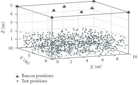
The algorithm’s behaviour depends mainly on the goodness of the distance estimations, but it is also influenced by the relative positions of the tags and beacons. The test-bench we chose was a 10×10 m room with eight beacons in the ceil-ing, which was 5 m high. As shown inFigure 3, four of them were placed at the corners and the rest inside the ceiling. As stated by Ray and Mahajan, this is not an optimal disposi-tion of the beacons if one wishes to avoid singularities [25]. However, these authors’ recommendations would lead to im-practical locations, as some of the beacons will be at floor level and their chirps will suffer significant blockage. Thus, the arrangement proposed in this paper is designed to pro-vide maximum ultrasonic coverage in the area in which the tags are to be located. In order to cover all the relative situa-tions of the tag and beacons, we took 1000 points distributed randomly in the room, up to 2 m high (Figure 3).
From each test point, we calculated their distances to the beacons; this was the input data free of errors. We calcu-lated several errors from the beacons’ coordinates and in-troduced them in the distances to test the algorithm. We then modelled the aforementioned situations in the follow-ing ways. The blockage of Type II was modelled addfollow-ing a distance-dependent, uniformly positive random error to all distances with a maximum value from 1% to 5%. The
Error 1 Error 2 Error 3 Error 5 (%) 0
0.05 0.1 0.15 0.2 0.25 0.3 0.35 0.4
Least squares LMedS
P
o
sitioning
er
ro
r
(m)
Figure4: Least-squares method versus LMedS method. Error A% indicates that all the distances used have a random uniform error with a maximum amplitude of A%.
errors of Type I followed a normal distribution, although their contribution was minor when there were NLOS errors present. Severe signal obstruction (Type III) was also simu-lated adding distance-dependent, uniformly positive random errors with maximum values of 10%, 50%, and 100%. The absence of data (Type IV) or the presence of clearly aberrant information from a beacon was not taken into account. Thus, when a distance was identified as wrong, it was directly dis-carded and not used as an input of the algorithm.
To obtain the final solution using LMedS method with 8 beacons, (7) shows that we will have 56 partial solutions to choose from. Although using a subset of the solutions could be useful, we used all of them to make the test as accurate as possible.
4.2. Definition of algorithm errors
Once we had chosen the evaluation scenario and the test cases that were to be applied to the different algorithms, we established the parameters that we were going to use to com-pare their behaviour. The most appropriate way to present the margin of error for each method was to use a confidence interval. Thus, we considered the statistical variable of “er-rors made” as the distance that separates the real point from the calculated one, in cm. The measurements taken were el-ements of the population (all the possible measurel-ements), and therefore a sample of the statistical variable to be stud-ied. Our aim was to evaluate the average of the error made, because this would indicate how exact the measurement was. In order to survey the interval limit of the average of the er-ror, that is, how exact the calculations were, we used the 99th percent confidence interval of the error made, in cm.
4.3. Comparison with other methods
com-Error 1% + 1 NLOS
Error 1% + 2 NLOS
Error 1% + 3 NLOS
Error 1% + 4 NLOS 0
0.1 0.2 0.3 0.4 0.5 0.6 0.7
Least-squares LMedS
P
o
sitioning
er
ro
r
(m)
(a)
Error 1% + 1 NLOS
Error 1% + 2 NLOS
Error 1% + 3 NLOS
Error 1% + 4 NLOS 0
0.5 1 1.5 2 2.5 3 3.5
Least-squares LMedS
P
o
sitioning
er
ro
r
in
(m)
(b)
Error 1% + 1 NLOS
Error 1% + 2 NLOS
Error 1% + 3 NLOS
Error 1% + 4 NLOS 0
1 2 3 4 5 6 7
Least-squares LMedS
P
o
sitioning
er
ro
r
in
(m)
(c)
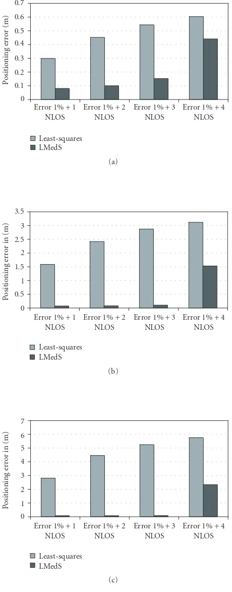
Figure 5: Least-squares method versus LMedS method. All the measurements have a random uniform error with a maximum am-plitude of 1%. Moreover,n of them have an NLOS error with a maximum amplitude of (a) 10%, (b) 50%, and (c) 100%, respec-tively.
pare the LMedS algorithm’s behaviour with the least-squares method.Figure 4shows the cases in which there were Type II errors in all beacons with several maximums: both algo-rithms show good behaviour in normal situations, even in shady environments with random errors of up to 5%.
Figure 5shows the cases in which one to four measure-ments were affected by heavy NLOS error (Type III). It is here that the LMedS algorithm demonstrates that it can manage NLOS errors effectively. While the least-squares algorithm fails even with NLOS errors of 10%, LMedS is able to han-dle up to three measurements with NLOS errors from a total of eight (which is quite improbable in a real situation), thus keeping the positioning error below 15 cm.
As stated in the introduction, Chen proposed a method with a similar approach that involves searching in a space of solutions [12]. A quantitative comparison is not possible be-cause the algorithm is in two dimensions and it is designed for GSM location with kilometric measurements of distance and standard errors of hundreds of meters. A qualitative comparison, on the other hand, is possible. The method pro-posed is not as precise as ours, since its error is far higher than the solution when only measurements without error are used, whereas we equaled it. This is because it does not elim-inate the aberrant solutions as we do, and all measurements have a weight in the final result.
4.4. Field test result
The positioning basics used in BLUPS also follow the mul-tilateration problem. The system consisted of beacons and tags, including Bluetooth modules (Mitsumi), which kept them sharply synchronized [13]. This, in combination with self-designed ultrasonic hardware (emitter and receiver), al-lowed the distances between beacons with known coordi-nates and tags to be measured. Then, with the data gathered, we calculated the tag position. The most significant contri-bution of this system is the remarkable relationship between the beacons (starting data) needed and the robustness and accuracy achieved. Other systems with similar features use many more beacons, but to achieve a margin of error of a few centimeters in a 10×10×5 m room, we only need five to eight beacons (in the hardest cases), while others require several dozens (one for every square meter) [27,28]. Hav-ing fewer beacons allows a large number of tags (more than 100) to be simultaneously positioned in the same room, at a refresh rate of 300 to 500 milliseconds (depending on the number of beacons used).
We evaluated BLUPS in various scenarios, but the most exhaustive analysis was performed at Malm¨o University, Swe-den. The installation had five beacons arranged in an area of 8×10 m with a height of 5 m. After 750 localizations in the room with direct vision of at least four beacons, we obtained a 99th percent confidence interval of the two-dimensional positioning error of ±3 cm, which rose to ±6 cm in three dimensions (3D).
However, the accuracy obtained makes it a good choice for static or low-motion location applications or for calibrating other systems. In another field test, we focused on guidance applications, for which it is necessary to obtain the orien-tation of the user in addition to the location. Analyzing the simultaneous position of two tags, the relative errors found were less than 1 cm in 3D, making tracking and head’s orien-tation very precise.
5. CONCLUSION
In this paper, we have presented an approach to NLOS error mitigation that adapts the robust least-median-of-squares (LMedS) method. It is well known that the best way of ensur-ing good positionensur-ing is to have redundant data usually settensur-ing more beacons than needed. The LMedS algorithm, far from simultaneously using all the available data, is based on mak-ing sets of input measurements that are used to obtain a space of solutions. The robust solution is the one that gives the least median of the squares of the errors. The LMedS method al-lows NLOS measurements to be rejected and gives accurate solutions even in rough conditions.
REFERENCES
[1] European Commission, “Directive 2002/58/EC on Privacy and Electronic Communications,” 2002.
[2] C. C. Docket, “Revision of the commission rule to ensure com-patibility with enhanced 911 emergency calling system,” Fed-eral Communications Commission Reports and Orders 96-264, Washington, DC, USA, 1996.
[3] K. Pahlavan, X. Li, and J. P. Makela, “Indoor geolocation science and technology,” IEEE Communications Magazine, vol. 40, no. 2, pp. 112–118, 2002.
[4] J. Borestein, H. R. Everett, and L. Feng,Where Am I? Sensors and Methods for Mobile Robot Positioning, University of Michi-gan, Ann Arbor, Mich, USA, 1996.
[5] P. Bahl and V. N. Padmanabhan, “RADAR: an in-building RF-based user location and tracking system,” inProceedings of 19th Annual Joint Conference of the IEEE Computer and Communi-cations Societies (INFOCOM ’00), vol. 2, pp. 775–784, Tel Aviv, Israel, March 2000.
[6] G. Anastasi, R. Bandelloni, M. Conti, F. Delmastro, E. Gregori, and G. Mainetto, “Experimenting an indoor bluetooth-based positioning service,” inProceedings of 23rd International Con-ference on Distributed Computing Systems Workshops (ICDCS ’03), pp. 480–483, Providence, RI, USA, May 2003.
[7] Ekahau Positioning Engine,http://www.ekahau.com. [8] I. Povescu, I. Nafomita, P. Constantinou, A. Kanatas, and N.
Moraitis, “Neural networks applications for the prediction of propagation pathloss in urban environments,” in Proceed-ings of 53rd IEEE Semi-Annual Vehicular Technology Conference (VTC ’01), vol. 1, pp. 387–391, Rhodes, Greece, May 2001. [9] W. Kim, G.-I. Jee, and J. Lee, “Wireless location with NLOS
error mitigation in Korean CDMA system,” inProceedings of the 2nd International Conference on 3G Mobile Communication Technologies, pp. 134–138, London, UK, March 2001. [10] S. Venkatraman and J. Caffery Jr., “Statistical approach to
non-line-of-sight BS identification,” inProceedings of the 5th Inter-national Symposium on Wireless Personal Multimedia Commu-nications, vol. 1, pp. 296–300, Honolulu, Hawaii, USA, Octo-ber 2002.
[11] S. Venkatraman, J. Caffery Jr, and H.-R. You, “Location using LOS range estimation in NLOS environments,” inProceedings of IEEE 55th Vehicular Technology Conference (VTC ’02), vol. 2, pp. 856–860, Birmingham, Ala, USA, 2002.
[12] P.-C. Chen, “A non-line-of-sight error mitigation algorithm in location estimation,” inProceedings of IEEE Wireless Commu-nications and Networking Conference (WCNC ’99), vol. 1, pp. 316–320, New Orleans, La, USA, September 1999.
[13] R. Casas, H. J. Gracia, A. Marco, and J. L. Falc ´o, “Synchroniza-tion in wireless sensor networks using Bluetooth,” in Proceed-ings of the 3rd International Workshop on Intelligent Solutions in Embedded Systems (WISES ’05), pp. 79–88, Hamburg, Ger-many, May 2005.
[14] W. H. Foy, “Position-location solutions by taylor-series esti-mation,”IEEE Transactions on Aerospace and Electronic Sys-tems, vol. 12, pp. 187–193, 1976.
[15] S. S. Ghidary, T. Tani, T. Takamori, and M. Hattori, “A new home robot positioning system (HRPS) using IR switched multi ultrasonic sensors,” inProceedings of IEEE International Conference on Systems, Man, and Cybernetics (SMC ’99), vol. 4, pp. 737–741, Tokyo, Japan, October 1999.
[16] A. Mahajan and M. Walworth, “3D position sensing using the differences in the time-of-flights from a wave source to vari-ous receivers,”IEEE Transactions on Robotics and Automation, vol. 17, no. 1, pp. 91–94, 2001.
[17] D. E. Manolakis, “Efficient solution and performance analysis of 3-D position estimation by trilateration,”IEEE Transactions on Aerospace and Electronic Systems, vol. 32, no. 4, pp. 1239– 1248, 1996.
[18] D. E. Manolakis and M. E. Cox, “Effect in range difference po-sition estimation due to stations’ popo-sition errors,”IEEE Trans-actions on Aerospace and Electronic Systems, vol. 34, no. 1, pp. 329–334, 1998.
[19] L. Girod and D. Estrin, “Robust range estimation using acous-tic and multimodal sensin,” inProceedings of IEEE/RSJ Inter-national Conference on Intelligent Robots and Systems (IROS ’01), vol. 3, pp. 1312–1320, Maui, Hawaii, USA, October-November 2001.
[20] D. Bohn, “Environmental effects on the speed of sound,” Jour-nal of the Audio Engineering Society, vol. 36, no. 4, pp. 223–231, 1988.
[21] Z. Zhang, “Parameter estimation techniques: a tutorial with application to conic fitting,” Rapport de recherche RR-2676, INRIA, Sophia-Antipolis, France, 1995.
[22] D. Mintz, P. Meer, and A. Rosenfeld, “Analysis of the least me-dian of squares estimator for computer vision applications,” inProceedings of IEEE Computer Society Conference on Com-puter Vision and Pattern Recognition (CVPR ’92), pp. 621–623, Champaign, Ill, USA, June 1992.
[23] P. J. Rousseeuw and A. M. Leroy,Robust Regression and Outlier Detection, John Wiley & Sons, New Yourk, NY, USA, 1987. [24] M. A. Fischler and R. C. Bolles, “Random Sample
Consen-sus: A Paradigm for Model Fitting with Applications to Image Analysis and Automated Cartography,”Communications of the ACM, vol. 24, no. 6, pp. 381–395, 1981.
[25] P. K. Ray and A. Mahajan, “Optimal configuration of receivers in an ultrasonic 3D position estimation system by using ge-netic algorithms,” inProceedings of the American Control Con-ference, vol. 4, pp. 2902–2906, Chicago, Ill, USA, June 2000. [26] R. L. Moses, D. Krishnamurthy, and R. M. Patterson, “A
[27] M. Addlesee, R. Curwen, S. Hodges, et al., “Implementing a sentient computing system,”IEEE Computer, vol. 34, no. 8, pp. 50–56, 2001.
[28] N. B. Priyantha, A. Chakraborty, and H. Balakrishnan, “The Cricket location-support system,” inProceedings of the 6th An-nual International Conference on Mobile Computing and Net-working (MobiCom ’00), pp. 32–43, Boston, Mass, USA, Au-gust 2000.
R. Casas is an Assistant Professor in the Electronic Engineering Department at the Technical University of Catalonia, Spain. His research interests include sensor net-works, digital electronics, and assistive tech-nology. He received an M.S. degree in elec-trical engineering in 2000 and a Ph.D. de-gree in electronic engineering in 2004, both from the University of Zaragoza.
A. Marcois an Assistant Professor in the Computer Science and Systems Engineering Department at the University of Zaragoza, Spain. His research interests include sensor networks, digital electronics, and assistive technology. He received an M.S. degree in electrical engineering in 2000 from the Uni-versity of Zaragoza, and is currently apply-ing to obtain a Ph.D. degree in electronic engineering.
J. J. Guerrero graduated in the Electrical Engineering Department at the University of Zaragoza in 1989. He obtained the Ph.D. degree in 1996 from the same institution, and currently he is an Assistant Professor at the Department of Computer Science and Systems Engineering. He gives lectures on control engineering, robotics, and 3D com-puter vision. His research interests are in the area of computer vision, particularly in
3D visual perception, photogrammetry, robotics, and vision-based navigation.