R E S E A R C H
Open Access
Optimal edge detection using multiple operators
for image understanding
Stamatia Giannarou
1*and Tania Stathaki
2Abstract
Extraction of features, such as edges for the understanding of aerial images, has been an important objective since the early days of remote sensing. This work aims at describing a new framework which allows for the quantitative combination of a preselected set of edge detectors based on the correspondence between their outcomes. This is inspired from the problem that despite the enormous amount of literature on edge detection techniques, there is no single technique that performs well in every possible image context. Two approaches are proposed for this purpose. The first approach is the well-known receiver operating characteristics analysis which is introduced for a sound quality evaluation of the edge maps estimated by combining different edge detectors. In the second approach, the so-called kappa statistics are employed in a novel fashion to amalgamate the above-mentioned selected edge maps to form an improved final edge image. This method is unique in the sense that the balance between the false detections (false positives and false negatives) is explicitly determined in advance and
incorporated in the proposed method in a mathematical fashion. For the performance evaluation of the proposed techniques, a sample set of the RADIUS/DARPA-IU Fort Hood aerial image database with known ground truth has been used.
1 Introduction
Automatic detection of both geographical (natural) and man-made structures, such as vegetation, buildings, roads and vehicles, in aerial or satellite images has been an active research topic the last decade [1,2]. Aerial images, with their highly detailed contents, are an important source of information for applications includ-ing GIS [3], traffic surveillance [4] and military applica-tions [5]. When processing aerial images, the extraction of high-level features for object detection is an impor-tant field. Features of interest can be extracted using a variety of image-processing techniques, which analyze the image to detect characteristics, such as edges, tex-ture and shape.
Edge-driven approaches have been extensively used in understanding remote sensing images and detecting man-made objects in them. In Noronha and Nevatia [6], extract edge points to build a system that detects and constructs 3D models of buildings using multiple aerial images. Tupin et al. [7] applied the ratio-of-averages (RoA) edge detector that was first presented by Touzi
et al. [8] to identify linear structures, such as main axes in road networks in synthetic aperture radar (SAR) images. In [9], a framework for automatic change detec-tion of linear features (e.g. roads and buildings) in aerial images is built, based on the edge maps which indicate pixels that segment areas with significantly different brightness values. Gamba et al. [10] proposed an approach to extract the map of urban areas exploiting edge information in very high-resolution images (VHR).
Edge detection in aerial images is a challenging task for many reasons. Aerial images differ in resolution, sen-sor type, orientation, quality, dynamic range, light condi-tions, different weather and seasons, factors that increase the complexity of the edge detection process. In several cases, some of the detected edges do not cor-respond to meaningful objects, while some edges that belong to objects are distorted, broken or missed. Furthermore, edges of different objects or edges of dif-ferent layers of a structure are likely to stick to each other. Edge detection must be efficient and reliable because it is crucial in determining how successful sub-sequent processing stages will be. To fulfill the reliability requirement of edge detection, a great diversity of
* Correspondence: [email protected]
1Hamlyn Centre for Robotic Surgery, Imperial College London, London, UK
Full list of author information is available at the end of the article
operators have been devised with differences in their mathematical and algorithmic properties.
Some of the earliest methods, such as the Sobel [11] and Roberts [12], are based on the so-called“ Enhance-ment and Thresholding“ approach [13]. According to that method, the image is convolved with small kernels which represent low-order high-pass filters and the result is thresholded to identify the edge points. Since then, more sophisticated operators have been developed. Marr and Hildreth [14] were the first to introduce the Gaussian smoothing as a pre-processing step in edge feature extraction. Their method detects edges by locat-ing the zero-crosslocat-ings of the Laplacian (second deriva-tive) of the output of a Gaussian filtered image. Canny [15] developed an alternative Gaussian edge detector based on the optimizing three criteria. He employed Gaussian smoothing to reduce noise and the first deriva-tive of the Gaussian to detect edges. Deriche [16] extended Canny’s work to derive a recursively imple-mented edge detector. Rothwell [17] designed a spatially adaptive operator which is able to recover reliable topo-logical information.
Further to the above, an alternative approach to edge detection is the multiresolution one. In such a detection framework, the image is convolved with Gaussian filters of different sizes to produce a set of images at different resolutions. These images are integrated to produce a complete final edge map. Typical algorithms which fol-low this approach have been produced by Bergholm [18], Lacroix [19] and Schunck [20]. Another interesting cate-gory of edge detectors is the logical/linear operators [21] which combine aspects of linear operators’theory and Boolean algebra. Furthermore, the idea of mimicking the human vision function using mathematical models gave space to the development of feature detection algorithms based on the human visual system. A representative example is the edge detector developed by Peli [22].
Recent approaches have used supervised learning to detect edges and object boundaries. In [23], a data-dri-ven statistical edge detection approach has been pro-posed, where the probability distributions of edge filter responsesonandoffedges are learnt from pre-segmen-ted data sets, while edges are detecpre-segmen-ted using the log-likelihood ratio test. In a similar spirit, Martin et al. [24] combine multiple local cues to detect local boundaries. Based on the brightness, color and texture features, a classifier is trained using pre-segmented data to model the true posterior probability of a boundary at every image location and orientation. Another supervised learning algorithm for edge detection is the boosted edge learning (BEL) [25]. In this approach, a large num-ber of features across different scales are combined to learn a discriminative model using an extended version
of the probabilistic Boosting tree classification algorithm.
Intuitively, the question that arises is which edge detector and detector parameter settings can produce optimal results. Despite the aforementioned volume of existing work, an ideal scheme able to detect and loca-lize edges with precision in many different contexts, has not yet been produced. Depending on the application, pre-segmented data might not be available for super-vised training. This is getting even more difficult because of the absence of an evident“correct”edge map (ground truth), on which the performance of an edge detector could be evaluated. Although an edge detector may be robust to noise, it may fail to mark corners and junctions properly. Another common issue with edge detection is the incomplete contour representation. Pro-blems, such as the above, strongly motivate the develop-ment of a general method for combining different edge detection schemes to take advantage of their strengths, while overcoming their weaknesses.
Let us assume noriginal detectors, where a detector refers to a mathematical method that attempts to iden-tify the presence (or absence) of an event. In our work, we are interested in edge detectors that investigate the presence of edges in a digital image signal. These origi-nal detectors are transformed to a new set of detectors, where each new detector is a function of all of the origi-nal detectors. This function is solely controlled by a parameter named correspondence threshold (CT) which will be explained in the main body of the paper. Each one of the new detectors is associated with a specific value of the CT parameter; this value identifies uniquely the detector. The new detectors vary with respect to their richness, starting from weak detectors that high-light only the strong edges and are basically noise free, to strong detectors that also highlight weak edges and fine details, but exhibit significant amount of noise. In this work, we are interested in selecting one of the new edge detectors as the final detection result. The method assumes that the best of the new edge maps is the one which is most consistent with the verity of the detec-tions produced by the set of original edge detectors. We present two novel contributions.
The second contribution is based on the employment of a normalized and corrected edge detection perfor-mance statistical metric known as kappa statistic. The kappa statistic has been used solely in medicine [27]. We are seeking at optimizing the kappa statistic which, in the specific framework, is a function of the available edge detectors and additionally a scalar parameter which con-trols the strength of the final detector and consequently the balance between false alarms and misdetections.
The later is the main novelty of this paper. It is an important research contribution to the edge detection problem, since it allows for the blind combination of multiple detectors and more importantly the pre-speci-fied control of the type of preferred misclassifications.
The work presented in this paper is a significant extension of the preliminary work presented in [28,29]. Two different contributions for optimal edge detection are studied in detail. Exhaustive experimental results are provided for assessing the relative strength of intrinsic technical merit of the proposed techniques for detecting edges in natural scenes. The proposed framework is compared against existing methods and their respective performance is evaluated on aerial images.
The paper is organized as follows. Section 2 concerns the brief analysis of a set of popular edge detectors that will be used in this work. Section 3 presents two novel approaches for the quantitative combination of multiple edge detectors. Section 4 contains experimental results yielded using our implementation of the automatic edge detection algorithms together with a comparative study of the methods’performance. Conclusions are given in Section 5.
2 Operators implemented for this work
Several approaches to edge detection focus their analysis on the identification of the best differential operator necessary to localize sharp changes of the image inten-sity. These approaches recognize the necessity of a preli-minary filtering step, as a smoothing stage, since differentiation amplifies all high-frequency components of the signal, including those of the textured areas and noise. The most widely used smoothing filter is the Gaussian one which has been shown to play an impor-tant role in detecting edges.
Canny’s approach [15] is a standard technique in edge detection. This scheme, in substance, identifies edges in the image as the local maxima of the convolution of the image with an“optimal” operator. The operator’s optim-ality is subject to three performance criteria defined by Canny and is a very close approximation to the first derivative of the two-dimensional Gaussian functionG (x,y). For example, the partial derivative with respect to xis defined as:
δ
δxG(x,y) =
δ δxe
−x22+yσ22
where s2 denotes the variance of the Gaussian filter and controls the degree of smoothing. After this pro-cess, candidate edge pixels are identified as the pixels that survive an additional thinning process known as nonmaximal suppression[15]. Then, the candidate edges are thresholded to keep only the significant ones. More-over, Canny suggestshysteresis thresholdingto eliminate streaking of edge contours.
Using an approach similar to Canny’s, Deriche [16] derived an alternative optimal operator. Contrary to Canny, whose operator is based on a finite antisym-metric filter, Deriche deals with an antisymantisym-metric filter which has an infinite support region defined as:
f(x) =−c·e−a|x|·sinωx
wherea,cand ωare positive real numbers. This filter is sharper than the derivative of the Gaussian and is effi-ciently implemented in a recursive fashion. The proce-dure that follows in Deriche’s method is the same as the one used in Canny’s edge detection; nonmaximal sup-pression and hysteresis thresholding are applied as described previously.
Although Canny’s detector performs well in localizing edges and suppressing noise; yet in several cases, it fails to provide a complete boundary in objects. Rothwell’s [17] operator is an improvement to earlier edge detec-tors, capable of recovering sound topological descrip-tions. It follows a line of work similar to Canny’s. The uniqueness of this algorithm originates in the use of a dynamic threshold which varies across the image [17].
In general, it is very difficult to find a single scale of smoothing which is optimal for all the edges in an image. One smoothing scale may keep good localiza-tion while giving deteclocaliza-tions sensitive to noise. Thus, multiscale edge detection is introduced as an alterna-tive. In this approach, edge detectors with different fil-ter sizes are applied to the image to extract edge maps at different smoothing scales. This information is then combined to result in a more complete final edge image.
In Lacroix [19] introduces another algorithm for multiscale detection based on Canny’s method. Con-trary to Bergholm [18] who proposed the tracking of edges from coarse-to-fine resolution, in Lacroix’s method the edge information is combined moving from fine-to-coarse resolution aiming at avoiding the problem of splitting edges. Schunck’s work [20] is another study that advocates the use of derivatives of Gaussian filters with different variances to detect intensity changes at different resolution scales. The gradient magnitudes over the selected range of scales are multiplied to amplify significant edges, while sup-pressing the weak ones. Hence, a composite edge image is formed.
In this work, we use the six edge detectors mentioned in this section. The use of convolution-based methods is justified by the fact that they are simple to implement, while producing accurate detection results.
3 Automatic edge detection
In this paper, we intend to throw light on the uncer-tainty associated with the parametric edge detection per-formance. The statistical approaches described here attempt to automatically form an optimum edge map, by combining edge images emerged from different detectors.
We begin with the assumption thatNdifferent edge detectors will be combined. The first step of the algo-rithm comprises the correspondence test of the edge images, Ei for i= 1, ..., N. A correspondence value is assigned to each pixel and is then stored in a separate array,V, of the same size as the initial image. The corre-spondence value is the frequency of identifying a pixel as an edge by the set of detectors. Intuitively, the higher the correspondence associated with a pixel, the greater the possibility for that pixel to be a true edge. Hence, the above correspondence value can be used as a reli-able measure to distinguish between true and false edges [26].
However, these data require specific statistical meth-ods to assess the accuracy of the resulted edge images-accuracy here being the extent to which detected edges agree with true edges. Correspondence values ranging from 0 to N produce N + 1 thresholds which corre-spond to edge detections with different combinations of true-positive and false-positive rates. The threshold that corresponds to correspondence value 0 is ignored. Hence, the main goal of the method is to estimate the correspondence threshold CT(from the set CTi where
i = 1, ..., N) which results in an accurate edge map that gives the finest fit to all edge images Ei. In this section, we describe two different approaches for this purpose.
3.1 ROC analysis
In our case, the classification task is a binary one includ-ing the actual classes {e, ne}, which stand for the edge and non-edge event, respectively and the predictive classes,predicted edgeand predicted non-edge, denoted by {E, NE}. Traditionally, the possible outcomes obtained by an edge detector are displayed graphically in a 2 × 2 matrix, theconfusion matrix.
To mathematically define the conditional probabilities in the confusion matrix, we begin by considering an image of size K×L. The probability of a pixel to be a true edge will be denoted as pk,l, wherek= 1, ...,Kand
l= 1, ...,L. In a similar way,qk,lwill represent the prob-ability of a pixel to be detected as edge. The probprob-ability of a true-positive outcome over all the pixels (k,l) of an image is defined as:
TP = Mean(pk,l·qk,l)
This leads to the following equation:
TP =P·Q+ρ·σp·σq (1)
where spand sq stand for the standard deviation of the distribution ofpk,l andqk,l, respectively. The para-meter P represents theprevalence which refers to the occurrence of true edge pixels in the image whereas, the level Q of the detection corresponds to the occurrence of pixels detected as edges [30]. The parameter r denotes the correlation coefficient betweenpk,landqk,l and its role is explained in detail in the Appendix. In this work, we assume that for a legitimate edge detec-tion the correladetec-tion coefficient between true and detected edges is positive. This is a realistic assumption since edge detection relies on mathematical methods that exploit the local edge intensity information. In the case of random edge detection, where the edges are identified purely by chance, the correlation coefficient is equal to r= 0. All the probabilities computed for legiti-mate and random edge detection are presented in the Appendix. Clearly, the optimum edge detector is the one that identifies as edges all the true edge pixels and therefore satisfies the equality:
P=Q (2)
identifying a true edge as edge pixel. It is also referred to as true-positive rate and is defined as follows:
SE = TPrate= TP
(TP + FN) (3)
The term specificity (SP) expresses the probability of identifying an actual non-edge as non-edge pixel. The measure 1 - SP is known as false-positive rate. These measures are given by the equations:
SP = TN(TN + FP)
or
FPrate= 1−TN
(TN + FP) (4)
Relying on the value of only one of the above metrics for edge detection accuracy estimation would be an oversimplification and will possibly lead to misleading inferences. Based on this idea, theROC analysis [32,33] can be introduced to quantify detection accuracy. In fact, aROCcurve provides a view of all the true-posi-tive/false-positive rate pairs emerged from varying the correspondence over the range of the observed data. In this work, the ROC curve is used to select the corre-spondence threshold CTthat would provide an opti-mum trade-off between the TPrateand the FPraterate of
edge detectors.
To calculate the points on the ROCcurve, we apply each correspondence thresholdCTi on the correspon-dence test outcome, i.e, the matrix Vmentioned above. This means the pixels are classified as edges and non-edges according to whether their correspondence value exceeds a CTi or not. Thus, we end up with a set of possible best edge mapsMj, forj= 1, ...,N, correspond-ing to each CTi. Each point on the ROC curve corre-sponds to the average match between all the initial edge maps and a possible best edge map. For that purpose, every Mj is compared to the set of the initial edge images,Ei, to calculate the true-positive,TPratej, and the false-positive,FPratej, rates associated with each of them. Hence, according to Equations 3 and 4, for theMjmap these rates are defined as:
TPratej= TPj
TPj+ FNj
(5)
FPratej = 1− TNj
FPj+ TNj
(6)
whereTPj+ FNjrepresents the average number of true
edges inMj.
Averaging in Equations 5 and 6 refers to the joint use of multiple edge detectors as shown in the following equations.
TPj=
1 N N i=1 1 K·L
K k=1 L l=1
MjE∩EiE
(7)
FNj=
1 N N i=1 1 K·L
K k=1 L l=1
MjNE∩EiE
(8)
where MjE and MjNErepresent the pixels detected as edges and non-edges in the edge mapMj, respectively. The same notation is used in the case of the edge maps Ei. The probabilitiesFPjandTNjare defined in a similar
way. For instance, the probability measurement in Equa-tion 7 indicates the average number of pixels detected as edges in Mjand match with edge pixels in all detec-tions Ei. Each edge map Mjgenerates a point (FPratej, TPratej) in theROC plane, forming theROC curve. The position of these points provides qualitative information about the detection accuracy of each edge map. As we mentioned in Equation 2, the optimumCT should cor-respond to a detection that gives prevalence value P equal to its level Q. By definition of true-positive and false-positive rate,P’· FPrate+P· TPrate=Q. This
defi-nition in conjunction with Equation 2 leads to the fol-lowing mathematical expression that the optimum ed ge detection should satisfy:
P·FPrate+P·TPrate=P (9)
Equation 9 defines a line that connects the points (0, 1) and (P,P) in theROC plane, known asdiagnosis line. Therefore, the optimum CT occurs at the intersection (or close to that) of theROC curve and the diagnosis line. The value of the selected CT determines how detailed the final edge image, EGT, will be. In the case of a noisy environment, the selection ofCT should give a trade-off between the increase in information provided by the final edge image and the decrease in noise.
3.2 Weighted kappa coefficient
In edge detection, it is prudent to consider the relative seriousness of each possible disagreement between true and detected edges when performing accuracy evalua-tion. This section is confined to the examination of an accuracy measure which is based on the acknowledge-ment that in detecting edges, depending on the specific application, the consequences of a false positive may be quite different from the consequences of a false nega-tive. For this purpose, the weighted kappa coefficient [34,35] is introduced for the estimation of the corre-spondence threshold that results in an optimum final edge map.
Consider a mathematical measure A0 of agreement
presence or absence of a condition. LetAc be the value expected on the basis of agreement by chance alone and Aa the value expected on the basis of complete agree-ment, i.e.,Aa= max{A0}. Based on the above definitions,
the kappa coefficient defined below is introduced as a correctedandnormalizedmeasure of agreement [35]:
k= A0−Ac Aa−Ac
(10)
In edge detection,A0 may be defined as a measure of
agreement between true and detected edges. The defini-tion ofAcandAais obvious.
A generalization of the above coefficient can be made to incorporate the relative cost of false positives and false negatives into the accuracy measure. We assume that weightswu,v, foru= 1, 2 andv= 1, 2, are assigned to the four possible outcomes of the edge detection pro-cess displayed in the confusion matrix. The weights indicate gain or cost and they lie in the interval 0≤|wu,
v|≤ 1. The observed weighted proportion of agreement is given as
D0w =
2 u=1 2 v=1
wu,vdu,v (11)
where du,v indicates the probabilities in the confusion matrix, calculated as shown in Table 1. Similarly, the chance-expected weighted proportion of agreement has the form
Dcw =
2 u=1 2 v=1
wu,vcu,v (12)
wherecu,vrefers to the above four probabilities, but in the case of random edge detection, i.e. the edges are identified purely by chance. Their analytic expression is given in Table 1. Based on the definition of kappa coef-ficient described previously, the weighted kappa coeffi-cient is then given by
kw=
D0w−Dcw max(D0w−Dcw)
(13)
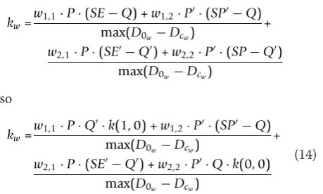
Substituting Equations 11 and 12 in Equations 13 gives
kw=
w1,1·P·(SE−Q) +w1,2·P·(SP−Q)
max(D0w−Dcw)
+
w2,1·P·(SE−Q) +w2,2·P·(SP−Q)
max(D0w−Dcw)
so
kw=
w1,1·P·Q·k(1, 0) +w1,2·P·(SP−Q)
max(D0w−Dcw)
+
w2,1·P·(SE−Q) +w2,2·P·Q·k(0, 0)
max(D0w−Dcw)
(14)
whereP’,Q’are the complements ofP andQ, respec-tively.k(1, 0) andk(0, 0) are the quality indices of sensi-tivity and specificity, respectively, defined as
k(1, 0) = SE−Q
Q and k(0, 0) =
SP−Q Q
The major source of confusion in statistical methods related to the weighted kappa coefficient is the assign-ment of weights. From Equation 14 it can be deduced that the total cost W1 for true edges being properly
identified as edges or not, is equal to W1 = |w1,1| + |
w2,1|. Similarly, the total cost W2for the non-edge pixels
is defined as W2= |w1,2| + |w2,2|. We propose that true
detections should be assigned positive weights repre-senting gain whereas, the weights for false detections should be negative, representing loss. It can be proven that no matter how the split of these total costs is made between true and false outcomes, the result of the method is not affected [30]. Hence, for the sake of con-venience, the total costs are split evenly. As a result, we end up with two different weights instead of four:
kw= W1
2 ·P·Q·k(1, 0) + (− W2
2 )·P·(SP−Q)
max(D0w−Dcw)
+
(−W12 )·P·(SE−Q) +W22 ·P·Q·k(0, 0) max(D0w−Dcw)
A further simplification leads to
kw=
W1·P·Q·k(1, 0) +W2·P·Q·k(0, 0)
max(D0w−Dcw)
(15)
Considering the fact that the maximum value of the quality indices k(1, 0) and k(0, 0) is equal to 1, the denominator in Equation 15 takes the form: W1·P ·Q’
+W2 ·P’·Q. Dividing both numerator and
denomina-tor by W1 +W2, the final expression of the weighted
kappa coefficient, in accordance with the quality indices of sensitivity and specificity, becomes
r·P·Q·k(1, 0) +r·P·Q·k(0, 0)
r·P·Q+r·P·Q =k(r, 0) (16)
Table 1 Probabilities for legitimate and random edge detection
Legitimate edge detection random edge detection
TP d1,1=P· SE c1,1=P·Q
FP d1,2=P’· SP’ c1,2=P’·Q
FN d2,1=P· SE’ c2,1=P·Q’
where
r= W1 W1+W2
(17)
and r’ is the complement of r. The weighted kappa coefficient k(r, 0) indicates the quality of the detection as a function ofr. It is unique in the sense that the bal-ance between the false detections is determined in advance and then is incorporated in the measure.
From Equation 17 it is deduced that the index r is indicative of the relative importance between false negatives and false positives. Its value is dictated by which type of error carries the greatest importance for a particular application and ranges from 0 to 1. If we focus on the elimination of false positives in edge detection, W2 will predominate in Equation 15 and
consequently r will be close to 0 as it can be seen from Equation 17. On the other hand, a choice of r close to 1 signifies our interest in avoiding false nega-tives since W1 will predominate in Equation 15. A
value of r = 1/2 reflects the idea that both false posi-tives and false negaposi-tives are equally unwanted. No standard choice of r can be regarded as optimum because the balance between the two errors shifts according to the application.
Thus, for a selected value of r, the weighted kappa coefficientkj(r, 0) is calculated for each edge map as in Equation 16. The optimum CTis the one that maxi-mizes the weighted kappa coefficient.
3.3 Geometric approach for the weighted kappa coefficient
The estimation of the weighted kappa coefficientkj(r, 0) can also be done geometrically. Every edge mapMj, for
j= 1 ... N, can be represented as a point (kj(0, 0), kj(1, 0)) on a two-dimensional graph with coordinates (k(0, 0),k(1, 0)). The set of points (kj(0, 0), kj(1, 0)),j= 1, ...,
N, consist the so-called quality ROC (QROC) curve. A great deal of information is available from visual exami-nation of such a geometric representation. Equation 16 for thejth edge map can be rewritten in the form:
kj(r, 0)−kj(1, 0)
kj(r, 0)−kj(0, 0)
=−P ·Q·r
P·Q·r (18)
Therefore, if we consider the straight line on the QROC-plane described by the equation:
kj(r, 0)−k(1, 0) =−
P·Q·r
P·Q·r(kj(r, 0)−k(0, 0)) (19) it is obvious from Equation 18 and 19 that the point (kj(0, 0),kj(1, 0)) lies on this line. This is called the
r-pro-jection lineand its slope is
s=−P ·Q·r
P·Q·r (20)
It is obvious that the point (kj(r, 0),kj(r, 0)) lies also on the r-projection line and also on the main diagonal described by equationk(0, 0) =k(1, 0).
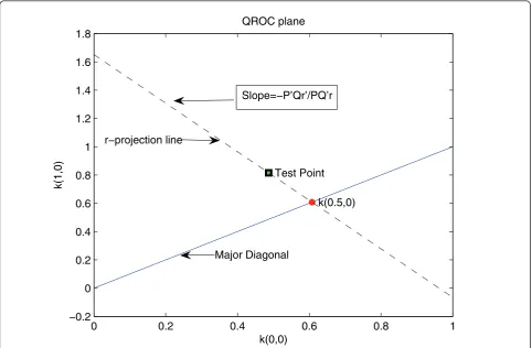
This means that the weighted kappa coefficient kj(r, 0) can be calculated graphically by drawing a line, for any valuer of interest, through the point (kj(0, 0), kj(1, 0)) with slope given by Equation 20. The intersection point, (kj(r, 0), kj(r, 0)), of this line with the major diagonal in theQROCplane is clearly indicative of thekj(r, 0) value. Figure 1 presents an example for the calculation of the weighted kappa coefficient for a test point for r = 0.5. The procedure is repeated for everyCTito generate N different intersection points. The closer the intersection point to the upper right corner (ideal point), the higher the value of the weighted kappa coefficient. Hence, the optimum correspondence threshold is the one that pro-duces an intersection point closer to the point (1, 1) in theQROCplane.
3.4 An alternative to the selection of therparameter value
In the previous section, parameterr is evaluated accord-ing to Equation 17. By assignaccord-ing more weight to the false detection, we want to eliminate the ratio in Equa-tion 17 yields the appropriate value of r. However, a more efficient analysis is necessary. An alternative analy-sis that justifies the previously described selection ofris presented in this section.
Our main concern is to examine the behavior of the quality measurek(r, 0) as a function of the level,Q, and the parameter r. Substituting in Equation 16 the prob-abilities given in the Appendix, the weighted kappa coef-ficient can be expressed as
k(r, 0) = r·P·Q
·k(1, 0) +r·P·Q·k(0, 0) r·P·Q+r·P·Q
= r·P·(SE−Q) +r·P·(SP−Q) r·P·Q+r·P·Q = r·P·(ρσpσq
P) +r·P·(ρσpσq
P) r·P·Q+r·P·Q
Thus, the quality measure,k(r, 0), takes the form
k(r, 0) = ρ·σp·σq r·P·Q+r·P·Q
The derivative of the weighted kappa coefficient with respect tor is given by
d
drk(r, 0) =ρσpσq·
Q−P
The measures sp,sq are positive as they express stan-dard deviations. The correlation coefficient,r, is posi-tive, as well. Thus, it becomes obvious that the sign of the the derivative,drdk(r, 0), is determined by the value ofQrelative to P.
A level,Q, greater than the prevalence,P corresponds to an edge detection that eliminates the misdetections by favoring the false positives. In this case, according to Equation 21, the derivative of the Weighted Kappa Coefficient is positive for any value ofr and the quality measure k(r, 0) is an increasing function of r. This means in applications where we are more interested in the elimination of false negatives, a higher value ofr in the interval [0, 1] will result in the selection of a more accurate edge map.
Equivalent conclusions are derived for the elimina-tion of false positives, i.e. detecelimina-tions where the level is smaller than the prevalence. According to Equation 21 the derivative, d
drk(r, 0), will be negative and the
weighted kappa coefficient will be a decreasing func-tion ofr. Therefore, small values ofr in the interval [0, 1] will yield CTs that correspond to more accurate edge maps.
The above conclusions are also verified experimen-tally. Figure 2 illustrates the values of the weighted kappa coefficient as a function ofr for four edge maps at different CTs. These plots are yielded from applying the weighted kappa coefficient method on the “School” image (from the RADIUS/DARPA-IU Fort Hood aerial image database [36]) to combine six edge detectors. Fig-ure 2a,b corresponds to CTs equal to 1 and 2, respec-tively, where the level values are greater than the prevalence. Observing these curves, it is clear that the weighted kappa coefficient is an increasing function ofr and high quality is achieved for values ofr close to 1. In contrast, as shown in Figure 2c,d, the quality measure is a decreasing function of r for CT = 3 and CT = 4, where the level is smaller than the prevalence. In this case, values of r close to 0 give edge maps with better quality.
4 Experimental results and discussion
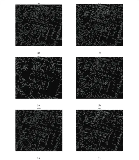
Using the above framework, six edge detectors, pro-posed by Canny [15], Deriche [16], Bergholm [18], Lacroix [19], Schunck [20] and Rothwell [17] were combined to produce optimum edge maps. The
0 0.2 0.4 0.6 0.8 1
−0.2 0 0.2 0.4 0.6 0.8 1 1.2 1.4 1.6 1.8
Test Point
k(0.5,0)
k(0,0)
k(1,0)
QROC plane
Slope=−P’Qr’/PQ’r
r−projection line
Major Diagonal
selection of the above edge detectors relies on the fact that they basically follow the same mathematical approach.
The performance evaluation study of the proposed approach is carried out on a set of 10 images, selected from the RADIUS/DARPA-IU Fort Hood aerial image set [36]. Some of the images contain mainly vertical views and others contain more oblique views as well. All the images are 8-bit/pixel and their size ranges from 476 × 477 to 645 × 667 pixels. The ground truth for the aer-ial images is provided in the data set [36], in the form of specified image points that should be identified as edges and specified image regions where no edges should be detected.
The performance of the edge detectors is evaluated with respect to two different measures; namely, the detection error and the similarity between the ground truth and the extracted edge maps. The detection error is defined as the distance of the (FPrate, TPrate) point of
the detector in the ROC plane from the ideal point (0, 1) and is mathematically expressed as:
Detection error =
(1−TPrate)2+ (FPrate)2 (22)
Equation 7 and 8. The similarity between the ground truth edge map and the result of an edge detector is estimated as:
Similarity = 1 NGT
NGT
i=1
1 1 +d2
i
(23)
where NGT is the number of edge points on the
ground truth and di is the minimum distance between the ith edge point on the ground truth and the esti-mated edge map. Intuitively, the lower the detection error and the higher the similarity to the ground truth, the better is the performance of the operator.
Specifying the value of the edge detection operators’ input parameters was a crucial step. In fact, the para-meter selection depends on the implementation and intends to maximize the quality of the detection. In our work, we were consistent with the parameters proposed by the authors of the selected detectors. The Bergholm algorithm was slightly modified by adding hysteresis thresholding to allow a more detailed result. In Lacroix technique, we applied non-maximal suppression by keeping the sizek× 1 of the relative window fixed at 3 ×1 [19]. For simplicity, in the case of Schunck edge detection, the non-maximal suppression method we used is the one proposed by Canny [15] and hysteresis thresholding was applied for a more efficient thresholding.
For all the images on the data set, the standard devia-tion (sigma) of the Gaussian filter in Canny’s algorithm [15] was set to sigma = 1, whereas, the low and high thresholdswere automatically calculated by the image histogram. In Deriche’s technique [16], the parameters’ values were set to a= 2 and w = 1.5. The Bergholm [18] parameter set was a combination ofstarting sigma, ending sigma and low and high threshold and these wherestarting sigma= 3.5,ending sigma = 0.7 and the thresholds were automatically determined as previously. For the Primary Rater in Lacroix’s method [19], the coarsest resolution was set tos2= 2 and the finest one
to s0 = 0.7. The intermediate scale s1 was computed
according to the expression proposed in [19]. The gradi-ent and homogeneity thresholds were estimated by the histogram of the gradient and homogeneity images, respectively. For the Schunck edge detector [20], the number of resolution scales was arbitrarily set to three as:s1 = 0.7,s2 = 1.2,s3 = 1.7. The difference between
two consecutive scales was selected not to be greater than 0.5 to avoid edge pixel displacement in the resulted edge maps. The values for the lowand high thresholds were calculated by the histogram of the gradient magni-tude image. In the case of Rothwell method [17], the alphaparameter was set to 0.9, the low threshold was estimated by the image histogram again and the value of
the smoothing parameter, sigma, was equal to 1. It is important to stress out that the selected values for all of the above parameters fall within the ranges proposed in the literature by the authors of the individual detectors.
When the optimum correspondence threshold is esti-mated using the maximization of the‘Weighted Kappa Coefficient’approach, the value of ther parameter needs to be set. The cost,r, is initially determined according to the particular quality of the detection (FP or FN) that is chosen to be optimized. For example, as far as target object detection in military applications is concerned, missing existing targets in the image (misdetections) is less desirable than falsely detecting non-existing ones (false alarms). This is as well the scenario we assume in this piece of work; namely, we are primarily concerned with the elimination of FN at the expense of increasing the number of FP. Therefore, according to the analysis in the previous section, the cost value r should range from 0.5 to 1.
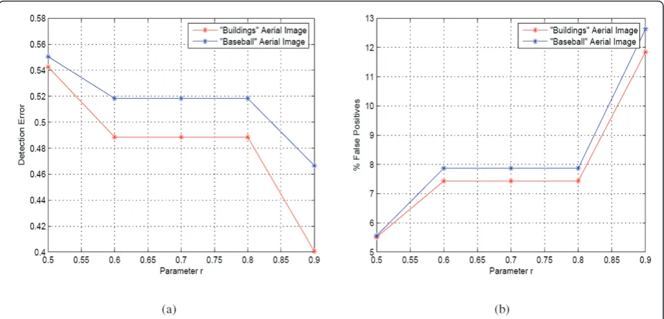
The graphs in Figure 3 show the detection error and the percentage of false positives for values of r greater than 0.5, for the “Buildings” and the “Baseball” aerial images. As it is expected, as the parameter rincreases, the detection error decreases, while the number of points falsely detected as edges increases. From the above graphs, it can be observed that a value of r between 0.6 and 0.8 gives a good trade-off between the increase in edge information and the decrease in noise in the final edge image. In our experimental work, the parameterrhas been set equal to 0.7.
The results of applying the ‘ROC analysis’ and the
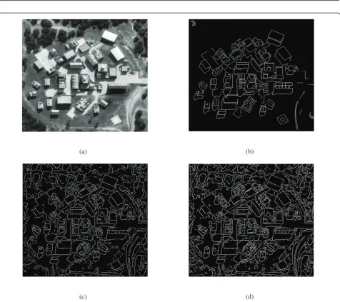
‘weighted kappa coefficient’ approach on the “Large Building”aerial image shown in Figure 4a are presented in Figures 4, 5, and 6. The sample space, Ei(i= 1, ..., 6), consisted of the edge detection out-comes produced by the six selected operators is depicted in Figure 5. The probabilities given by Equation 5 and 6 were calculated for the statistical correspondence test of the edge detec-tionsEi. The ROC curve implementation is illustrated in Figure 6a where it can be observed that the intersection of the diagnosis line with the ROC curve occurs at a correspondence level close to 3. Thus, the optimum threshold for this approach is CT = 3. The graphical estimation of the weighted kappa coefficient,kj(r, 0), for eachCT is illustrated in Figure 6b. On the graph, it is observed that the weighted kappa coefficient takes its maximum value at k2(r, 0) and therefore the optimum
CTis equal to 2. The final edge maps, EGT, for both approaches are presented in Figure 4c,d.
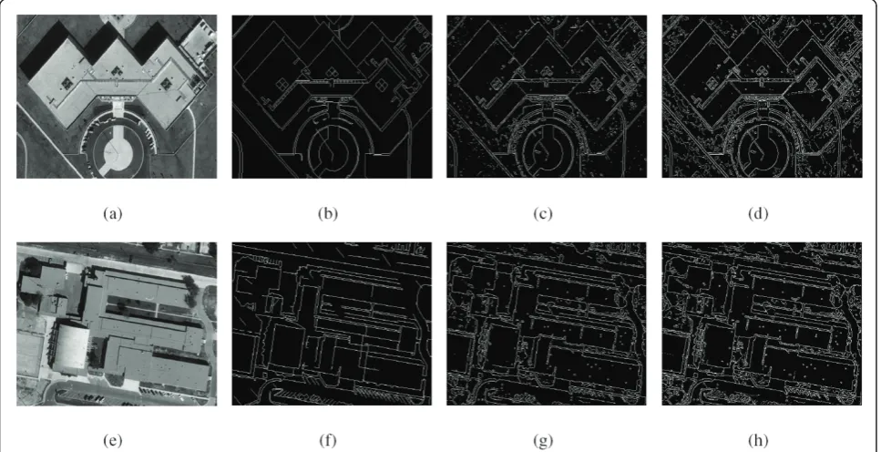
implementation and the graphical estimation of the weighted kappa coefficient are presented in Figure 9 giv-ing an estimation for the optimum CT for each approach equal to 3 and 2, respectively. The final edge maps for the ’ROC analysis’and the ‘weighted kappa coefficient’approach are presented in Figure 7c,d. The results of applying the proposed approaches to optimal edge detection on the“Main Building”and the“School” images are presented in Figure 10.
The above examples emphasize the ability of the approaches to combine high accuracy with good noise reduction in the final edge detection result. Insignificant information is cleared, while the one preserved allows for easy, fast and accurate object recognition. Further-more, it is interesting to note that objects missed by one of the selected edge detectors are included in the final edge image. This is particularly obvious in the “Large Building” image set when comparing the final edge maps in Figure 4c,d with the Bergholm detection in Fig-ure 5c. Finally, edges due to textFig-ure are suppressed in the final edge maps.
Comparing the edge maps produced by applying the above two approaches it is observed that the edge maps for the “weighted kappa coefficient”approach have bet-ter quality than those for the “ROC analysis”. The objects detected by the “weighted kappa coefficient” approach are better defined regarding their shape and contour and the number of detected edges is greater. This is expected since the selected value ofris 0.7. The
performance of the “weighted kappa coefficient” approach for the particular choice of r, seems to be superior to“ROC analysis” since it is more sensitive to minor details.
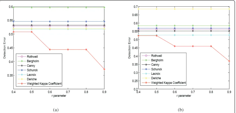
To investigate the effect of the costr on the detection error, the latter measurement was evaluated for both of the above aerial images, for different values ofr, greater than 0.4. The results for the “Large Building” and the
“Woods”images are graphically presented in Figure 11. The curves that correspond to the six edge detectors are straight lines parallel to the horizontal axes as the detec-tion result for these operators is not affected by the parameterr. From the graphs, it is clear that the detec-tion error for the‘weighted kappa coefficient’approach is lower than that of the six selected detectors for any value of r in the examined range. This observation shows that our experimental results are not biased by the selection of the parameter r since the ‘weighted kappa coefficient’approach is superior to the selected detectors for any value of r that eliminates the FN (r >0.5).
equal to 0.7, is always better than all the other approaches. The performance of the‘ROC analysis’ is lower than that of the ‘weighted kappa coefficient’ approach but better than that of the six selected opera-tors for the majority of the examined aerial images. The above results verify the superiority of the proposed approaches against the initial set of edge detectors.
Without code optimization, the MATLAB implemen-tation of each of the proposed approaches ("ROC analy-sis” and the“weighted kappa coefficient”) comfortably runs at around 2.8 s on a Pentium 2.8 GHz desktop for a 476 × 477 size image.
5 Conclusion
Figure 6Graphical estimation of the optimum CT for the“Large Building”aerial image when applying (a) the“ROC analysis”(b) “Weighted Kappa Coefficient”approach withr= 0.70.
weighted kappa coefficient approach can be considered superior in the sense that the trade off between detec-tion of minor edges and noise reducdetec-tion can be quanti-fied in advance as part of the problem specifications.
In future work, we intent to incorporate in the identi-fication of edges information from their surrounding pixels. That means, the probability of a pixel being an edge will be affected by the state (edge/non-edge) of its neighbors. Furthermore, the possibility of using soft Figure 9Graphical estimation of the optimum CT for the“Woods”aerial image when applying (a) the“ROC analysis”(b)“Weighted Kappa coefficient”approach withr= 0.70.
Figure 11Detection error with respect to the value of therparameter for (a) the“Large Building”image (b) the“Woods”image.
Table 2 Detection error
Rothwell Bergholm Canny Schunck Lacroix Deriche ROC Weighted kappa coeff. (r= 0.7)
Buildings 0.5506 0.6047 0.5593 0.5640 0.5736 0.5500 0.5425 0.4885
Baseball 0.5710 0.5968 0.5668 0.5689 0.5865 0.5726 0.5505 0.5183
Airfield 0.4707 0.4643 0.5057 0.5147 0.5340 0.5276 0.4634 0.4126
Homes 0.5991 0.5703 0.5712 0.5743 0.4851 0.6302 0.5177 0.4402
Large building 0.5292 0.5970 0.5328 0.5459 0.5180 0.5194 0.5084 0.4440
Main building 0.5608 0.5651 0.6180 0.6130 0.5193 0.6677 0.5439 0.4561
Pool tennis 0.5273 0.5639 0.5086 0.5367 0.5396 0.4852 0.5029 0.4343
School 0.5638 0.5844 0.5571 0.5647 0.5701 0.5928 0.5444 0.5001
Series 0.4321 0.5297 0.4143 0.4276 0.4522 0.5303 0.4139 0.3619
Woods 0.5634 0.5846 0.5526 0.5695 0.5274 0.6856 0.5241 0.4602
Table 3 Edge map similarity
Rothwell Bergholm Canny Schunck Lacroix Deriche ROC Weighted kappa coeff. (r= 0.7)
Buildings 0.6886 0.5895 0.6892 0.6804 0.6570 0.6871 0.6946 0.7355
Baseball 0.6815 0.6359 0.6961 0.6848 0.6579 0.6934 0.6995 0.7249
Airfield 0.7692 0.7651 0.7593 0.7382 0.7162 0.7516 0.7760 0.8492
Homes 0.6332 0.5978 0.6851 0.6762 0.7143 0.6169 0.7064 0.7599
Large building 0.6844 0.5401 0.6976 0.6730 0.6823 0.7082 0.7014 0.7506
Main building 0.6967 0.6191 0.6612 0.6499 0.6988 0.6088 0.6998 0.8357
Pool tennis 0.6722 0.5923 0.7208 0.6596 0.6527 0.7100 0.7046 0.7639
School 0.6495 0.5846 0.6743 0.6474 0.6419 0.6458 0.6669 0.7835
Series 0.7577 0.6084 0.7682 0.7656 0.7259 0.6810 0.7767 0.8090
values for the final edge maps instead of hard edge extractors will be explored.
Appendix
Correlation coefficient between the probability of a pixel being a true edge and being detected as edge
The parameterrin Equation 1 denotes the correlation coefficient between the probability of a pixel being a true edge and being detected as edge. A positive correla-tion coefficient between two random variables indicates that these variables follow the same trend. In our case, the random variables of interest are the true edge image and the detected edge image. Therefore, a positive cor-relation coefficient indicates that if the probability of a pixelf(x1,y1) being a true edge is higher as compared to
the same probability for the pixel f(x2, y2), then the
probability of the pixelf(x1,y1) detected as edge pixel is
also higher compared with the same probability for the pixelf(x2,y2).
All the probabilities, computed for legitimate and ran-dom edge detection, according to Equation 1 are pre-sented in Table 4 where the ‘ symbol denotes the complement operator.
Acknowledgements
The investigations which are the subject of this paper were initiated by Dstl under the auspices of the United Kingdom Ministry of Defence Systems Engineering for Autonomous Systems Defence Technology Centre.
Author details
1Hamlyn Centre for Robotic Surgery, Imperial College London, London, UK 2Department of Electrical and Electronic Engineering, Imperial College
London, South Kensington Campus, SW7 2AZ, UK
Competing interests
The authors declare that they have no competing interests.
Received: 7 February 2011 Accepted: 23 July 2011 Published: 23 July 2011
References
1. EP Baltsavias, Object extraction and revision by image analysis using existing geodata and knowledge: current status and steps towards operational systems. ISPRS J Photogram Remote Sens.58, 129–151 (2004). doi:10.1016/j.isprsjprs.2003.09.002
2. A Gruen, O Kuebler, P Agouris,Automatic Extraction of manmade Objects from Aerial and Space Images I(Birkhaeuser, Basel 1995)
3. K Zhang, J Yan, SC Chen, Automatic construction of building footprints from airborne lidar data. IEEE Trans Geosci Remote Sens.44(9), 2523–2533 (2006)
4. JM Munoz-Ferreras, F Perez-Martinez, J Calvo-Gallego, A Asensio-Lopez, BP Dorta-Naranjo, A Blanco del Campo, Traffic surveillance system based on a high-resolution radar. IEEE Trans Geosci Remote Sens.46(6), 1624–1633 (2008)
5. P Robertson, JM Brady, Adaptive image analysis for aerial surveillance. IEEE Intell Syst Appl.14(3), 30–36 (1999). doi:10.1109/5254.769882
6. S Noronha, R Nevatia, Detection and modeling of buildings from multiple aerial images. IEEE Trans Pattern Anal Mach Intell.23(5), 501–518 (2001). doi:10.1109/34.922708
7. F Tupin, H Maitre, J-F Mangin, J-M Nicolas, E Pechersky, Detection of linear features in sar images: application to road network extraction. IEEE Trans Geosci Remote Sens.36(2), 434–453 (1998). doi:10.1109/36.662728 8. R Touzi, A Lopes, P Bousquet, A statistical and geometrical edge detector
for SAR images. IEEE Trans Geosci Remote Sens.26(6), 764–773 (1988). doi:10.1109/36.7708
9. NC Rowe, LL Grewe, Change detection for linear features in aerial photographs using edge-finding. IEEE Trans Geosci Remote Sens.39(7), 1608–1612 (2001). doi:10.1109/36.934092
10. P Gamba, F Dell’Acqua, G Lisini, G Trianni, Improved VHR urban area mapping exploiting object boundaries. IEEE Trans Geosci Remote Sens. 45(8), 2676–2682 (2007)
11. J Matthews, An introduction to edge detection: the Sobel edge detector Available at http://www.generation5.org/content/2002/im01.asp (2002) 12. LG Roberts,Machine perception of 3-D solids. Optical and Electro-Optical
Information Processing (MIT Press, cambridge, 1965)
13. IE Abdou, WK Pratt, Quantitative design and evaluation enhancement/ thresholding edge detectors. Proc IEEE.67, 753–763 (1979)
14. D Marr, EC Hildreth, Theory of edge detection. Proc R Soc Lond.B207, 187–217 (1980)
15. JF Canny, A computational approach to edge detection. IEEE Trans Pattern Anal Mach Intell.8(6), 679–698 (1986)
16. R Deriche, Using Canny’s criteria to derive a recursive implemented optimal edge detector. Int J Comput Vis.1(2), 167–187 (1987). doi:10.1007/ BF00123164
17. CA Rothwell, JL Mundy, W Hoffman, VD Nguyen, Driving vision by topology. In International Symposium on Computer Vision (Coral Gables, FL, 1995), pp. 395–400
18. F Bergholm, Edge focusing. IEEE Trans Pattern Anal Mach Intell.9(6), 726–741 (1995)
19. V Lacroix, The primary raster: a multiresolution image description, in
Proceedings 10th International Conference on Pattern Recognition.1, 903–907 (1990)
20. BG Schunck, Edge detection with Gaussian filters at multiple scales. In: Proceedings IEEE Computer Society Workshop on Computer Vision, 208–210 (1987)
21. LA Iverson, SW Zucker, Logical/linear operators for image curves. IEEE Trans Pattern Anal Mach Intell.17(10), 982–996 (1995). doi:10.1109/34.464562 22. E Peli, Feature detection algorithm based on visual system models. Proc
IEEE.90, 78–93 (2002). doi:10.1109/5.982407
23. S Konishi, AL Yuille, JM Coughlan, SC Zhu, Statistical edge detection: learning and evaluating edge cues. IEEE Trans Pattern Anal Mach Intell. 25(1), 57–74 (2003). doi:10.1109/TPAMI.2003.1159946
24. DR Martin, CC Fowlkes, J Malik, Learning to detect natural image boundaries using local brightness, color, and texture cues. IEEE Trans Pattern Anal Mach Intell.26(5), 530–549 (2004). doi:10.1109/ TPAMI.2004.1273918
25. P Dollar, T Zhuowen, S Belongie, Supervised learning of edges and object boundaries. In: IEEE Computer Society Conference on Computer Vision and Pattern Recognition (CVPR).2, 1964–1971 (2006)
26. Y Yitzhaky, E Peli, A method for objective edge detection evaluation and detector parameter selection. IEEE Trans Image Process.25(8), 1027–1033 (2003)
27. HC Kraemer, VS Periyakoil, A Noda, Tutorial in biostatistics: kappa coefficients in medical research. Stat Med.21(14), 2109–2129 (2002). doi:10.1002/sim.1180
28. S Giannarou, T Stathaki, Edge detection using quantitative combination of multiple operators. inIEEE Workshop on Signal Processing Systems Design and Implementation, 359–364 (2005)
29. S Giannarou, T Stathaki, Novel statistical approaches to the quantitative combination of multiple edge detectors. inInternational Conference on Image Analysis and Recognition (ICIAR), 184–195 (2006)
Table 4 Analytic form of probabilities for legitimate and random edge detection
Legitimate edge detection Random edge detection
TP P·Q+r·sp·sq=P· SE P·Q
30. HC Kraemer,Evaluating Medical Test: Objective and Quantitative Guidelines. (Saga Publications, Newbury Park, 1992)
31. BR Kirkwood, Jonathan AC Sterne,Essential Medical Statistics. (Blackwell Science, Oxford, 2003)
32. T Fawcett, ROC graphs: notes and practical considerations for data mining researchers. HP Labs Tech Report HPL-2003-4 (2003)
33. MH Zweig, G Campbell, Receiver-operating characteristic (ROC) plots: a fundamental evaluation tool in clinical medicine. Am Assoc Clin Chem. 39(4), 561–577 (1993)
34. JL Fleiss,Statistical Methods for Rates and Proportions(Wiley, New York, 1981)
35. J Sim, CC Wright, The kappa statistic in reliability studies: use, interpretation, and sample size requirements. J Am Phys Therapy,85(3), 257–268 (2005) 36. http://marathon.csee.usf.edu/edge/edgecompare_main.html
doi:10.1186/1687-6180-2011-28
Cite this article as:Giannarou and Stathaki:Optimal edge detection
using multiple operators for image understanding.EURASIP Journal on Advances in Signal Processing20112011:28.
Submit your manuscript to a
journal and benefi t from:
7Convenient online submission 7Rigorous peer review
7Immediate publication on acceptance 7Open access: articles freely available online 7High visibility within the fi eld
7Retaining the copyright to your article