Digital IIR Filter Design Using Differential
Evolution Algorithm
Nurhan Karaboga
Department of Electronic Engineering, Faculty of Engineering, Erciyes University, 38039 Melikgazi, Kayseri, Turkey Email:nurhan [email protected]
Received 14 May 2004; Revised 3 December 2004; Recommended for Publication by Ulrich Heute
Any digital signal processing algorithm or processor can be reasonably described as a digital filter. The main advantage of an infinite impulse response (IIR) filter is that it can provide a much better performance than the finite impulse response (FIR) filter having the same number of coefficients. However, they might have a multimodal error surface. Differential evolution (DE) algorithm is a new heuristic approach mainly having three advantages; finding the true global minimum of a multimodal search space regardless of the initial parameter values, fast convergence, and using a few control parameters. In this work, DE algorithm has been applied to the design of digital IIR filters and its performance has been compared to that of a genetic algorithm.
Keywords and phrases:digital IIR filter, design, evolutionary algorithms, differential evolution, genetic algorithm.
1. INTRODUCTION
Anything that contains information can be considered as a signal. Therefore, signals arise in almost every field of science and engineering. Two general classes of signals can be iden-tified, namely, continuous-time and discrete-time signals. A discrete-time signal is one that is defined at discrete instants of time. The numerical manipulation of signals and data in discrete-time signals is called digital signal processing (DSP). The extraordinary growth of microelectronics and comput-ing has had a major impact on DSP. Therefore, DSP has al-ready moved from being primarily a specialist research topic to a one with practical applications in many disciplines. Al-most any DSP algorithm or processor can reasonably be de-scribed as a filter. Filtering is a process by which the frequency spectrum of a signal can be modified, reshaped, or manipu-lated according to some desired specifications. Digital filters can be broadly classified into two groups: recursive and non-recursive. The response of nonrecursive (FIR) filters is de-pendent only on present and previous values of the input signal. However, the response of recursive (IIR) filters de-pends not only on the input data but also on one or more previous output values. The main advantage of an IIR filter is that it can provide a much better performance than the FIR filter having the same number of coefficients. Design of a digital filter is the process of synthesizing and implement-ing a filter network so that a set of prescribed excitations re-sults in a set of desired responses [1,2]. However, there are some problems with the design of IIR filters [3,4,5]. The fundamental problem is that they might have a multimodal error surface. A further problem is the possibility of the filter
Initialization Evaluation
REPEAT
Mutation Recombination Evaluation Selection
UNTIL(termination criteria are met)
Algorithm1: Basic DE algorithm.
In this work, the performance comparison of the design methods based on DE and GA is presented for digital IIR filters since DE algorithm is very similar to, but much sim-pler than, GA. The paper is organized as follows. Section 2
presents a basic DE algorithm.Section 3describes the prob-lem. InSection 4, firstly the performance of DE is compared with that of GA on a set of well-known numeric test func-tions [19] and secondly, DE and GA are applied to the design of low- and high-order digital IIR filters and the results ob-tained are discussed.
2. DIFFERENTIAL EVOLUTION ALGORITHM
An optimization task consisting ofDparameters can be rep-resented by aD-dimensional vector. In DE, a population of
NP solution vectors is randomly created at the start. This population is successfully improved by applying mutation, crossover, and selection operators.
The main steps of a basic DE algorithm is given in
Algorithm 1. 2.1. Mutation
For each target vectorxi,G, a mutant vector is produced by
vi,G+1=xi,G+K
xr1,G−xi,G
+Fxr2,G−xr3,G
, (1)
wherei,r1,r2,r3 ∈ {1, 2,. . .,NP}that are randomly chosen and must be different from each other. In (1),Fis the scaling factor belonging to [0, 2] affecting difference vector (xr2,G− xr3,G),Kis the combination factor.
2.2. Crossover
The parent vector is mixed with the mutated vector to pro-duce trial vector
Uji,G+1=
vji,G+1
ifrndj≤CR
or j=rni, xji,G if
rndj> CR
and j=rni,
(2)
where j = 1, 2,. . .,D;rj ∈ [0, 1] is the random number; CR stands for the crossover constant ∈ [0, 1]; and rni ∈
(1, 2,. . .,D) is the randomly chosen index.
2.3. Selection
Performance of the trial vector and its parent is compared and the better one is selected. This method is usually named greedy selection. All solutions have the same chance of be-ing selected as parents without dependence on their fitness
value. The better one of the trial solution and its parent wins the competition providing significant advantage of converg-ing performance over genetic algorithms.
3. DEFINITION OF THE PROBLEM
Consider the IIR filter with the input-output relationship governed by
y(k) +
M
i=1
biy(k−i)= L
i=0
aix(k−i), (3)
wherex(k) andy(k) are the filter’s input and output, respec-tively, andM(≥L) is the filter order. The transfer function of this IIR filter can be written in the following general form:
H(z)=A(z)
B(z)=
L i=0aiz−i
1 +Mi=1biz−i
. (4)
Hence, the design of this filter can be considered as an opti-mization problem of the cost functionJ(w) stated as follows:
min
w∈WJ(w), (5)
where w = [a0a1· · ·aLb1· · ·bM]T is the filter coefficient
vector.
The aim is to minimize the cost functionJ(w) by adjust-ing w. The cost function is usually expressed as the time-averaged cost function defined by (4):
J(w)= 1 N
N
k=1
d(k)−y(k)2, (6)
where d(k) and y(k) are the filter’s desired and actual re-sponses of the filter, respectively, and N is the number of samples used for the calculation of the cost function.
4. SIMULATION RESULTS
In this section, firstly the performance of DE algorithm is compared to that of the well-known models of GA, Grefenstette [20], Eshelman et al. [21], and M¨uhlenbein et al. [22], on a set of numeric test functions defined by De Jong [19], and secondly, the algorithms are applied to the design of IIR filters for the purpose of system identification.
4.1. Numeric function optimization
Table1: Test functions.
Function number Function Limits
F1
3
i=1 x2
i −5.12≤xi≤5.12
F2 100x2
1−x2
2
+1−x1
2
−2.048≤xi≤2.048
F3
5
i=1
integerxi
−5.12≤xi≤5.12
F4
30
i=1 ix4
i + Gauss(0, 1) −1.28≤xi≤1.28
F5
0.002 +
25
j=1
1 j+2i=1
xi−ai j
6
−1
−65.536≤xi≤65.536
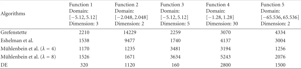
Table2: Average evaluation numbers.
Algorithms
Function 1 Domain: [−5.12, 5.12] Dimension: 3
Function 2 Domain: [−2.048, 2.048] Dimension: 2
Function 3 Domain: [−5.12, 5.12] Dimension: 5
Function 4 Domain: [−1.28, 1.28] Dimension: 30
Function 5 Domain: [−65.536, 65.536] Dimension: 2
Grefenstette 2210 14229 2259 3070 4334
Eshelman et al. 1538 9477 1740 4137 3004
M¨uhlenbein et al. (λ=4) 1170 1235 3481 3194 1256
M¨uhlenbein et al. (λ=8) 1526 1671 3634 5243 2076
DE 320 1120 160 2800 1500
F1 (Sphere)
The first function is smooth, unimodal, strongly convex, and symmetric.
F2 (Banana)
Rosenbrock’s valley is a classic optimization function, also known as Banana function. The global optimum is inside a long, narrow, parabolic-shaped flat valley. To find the val-ley is trivial; however, convergence to the global optimum is difficult and hence this problem has been repeatedly used to assess the performance of optimization algorithms.
F3 (Step)
This function represents the problem of flat surfaces. Flat surfaces are obstacles for optimization algorithms because they do not give any information about which direction is favourable. Unless an algorithm has variable step sizes, it can get stuck on one of the flat plateaus.
F4 (Stochastic)
This is a simple unimodal function padded with noise. In this type function, the algorithm never gets the same value on the same point. Algorithms not doing well on this test function will do poorly on noisy data.
F5 (Foxholes)
Function F5 is an example of a function with many local op-tima. Many standard optimization algorithms get stuck in the first peak they find.
The DE algorithm has a few control parameters: num-ber of population NP, scale vector F, combination coeffi -cient K, and crossover rate CR. The problem-specific pa-rameters of DE algorithm are maximum generation number
Gmax and number of parameters defining problem dimen-sion D. The values of these two parameters depend on the problem to be optimized. The average evaluation numbers providing the minimum values of test functions in three-digit accuracy have been presented inTable 2. In this work, first the performance of DE algorithm was compared to that of GAs described by Grefenstette [20], Eshelman et al. [21], and M¨uhlenbein et al. [22]. DE algorithm was run 50 times for each function. For every run, the initial population was randomly created by means of using different seed numbers. The results belonging to DE algorithm inTable 2 were achieved using the following parameter values: population size = 50, crossover rate = 0.8, scaling factor= 0.8, and combination factor=0.8. From the results obtained by using GAs and DE, it is easy to see that the DE algorithm is usually able to find similar solutions for the test functions with less number of evaluations.
4.2. Digital IIR filter design
DE algorithm IIR filter
Unknown plant
x(k)
y(k)
− +
e(k) d(k)
Figure1: Block diagram of the system identification process using IIR filter designed by the DE algorithm.
a0 a1 . . . aL b1 b2 . . . bM
Figure2: Representation of the parameters in the string form.
adjusted by the DE algorithm until the error between the out-put of the filter and the unknown system is minimized. By constraining the range of the filter coefficients, the stability is guaranteed. The filter coefficients are encoded in the string form as shown inFigure 2.
The fitness value of a solutioniin the population is de-termined by using the following formula:
fit(i)= 1
1 +J(w)i
, (7)
whereJ(w)iis the cost function value computed for the
solu-tioni. The first two examples (low-order IIR filters) used in the simulation studies were taken from [4,5,6,7,8,9,10,11,
12,13,14,15,16,17,18,19,20,21,22,23].
Example1. In the first example, the unknown plant and the filter had the following transfer functions:
Hz−1= 1
1−1.2z−1+ 0.6z−2,
HM
z−1= 1
1−a1z−1−a2z−2.
(8)
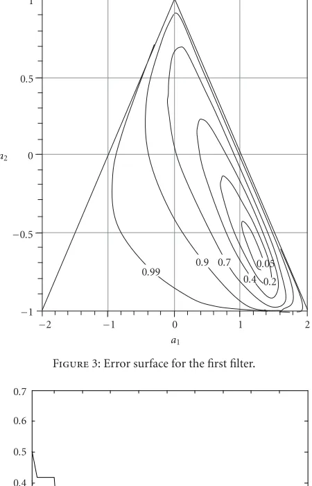
The input,x(k), to the system and the filter was a white se-quence. Since the filter order is equal to the system order, a local-minima problem does not occur. Figure 3 presents the error surface for this filter.Figure 4shows the evolution of the mean square error (MSE) averaged over 50 different runs of the DE. Each run had a randomly chosen initialw.
Figure 5also demonstrates the evolution of parameters for a run.
The effect of the control parameters on the DE algo-rithm’s performance was studied by Price [24]. The param-eter values used in this study were selected according to the recommended values in that work. Also, in order to carry out the comparison of the algorithms in similar conditions, the values of similar control parameters of the algorithms were chosen to be equal to each other; for example, population
a1
−2 −1 0 1 2 a2
−1 −0.5 0 0.5 1
0.99 0.9 0.7 0.4 0.2
0.05
Figure3: Error surface for the first filter.
5 10 15 20 25 30 35 40 45 50
Generation 0
0.1 0.2 0.3 0.4 0.5 0.6 0.7
Er
ro
r
DE GA
Figure4: Cost function value versus number of evaluations aver-aged over 50 random runs for DE and GA.
size, generation number, and crossover rate. Table 3shows the control parameter values used for both algorithms in IIR filter design.
Example2. In the second example, the plant was a second-order system and the filter was a first-second-order IIR filter with the following transfer functions:
Hz−1= 0.05−0.4z−1 1.0−1.1314z−1+ 0.25z−2,
HM
z−1= b 1−az−1.
5 10 15 20 25 30 35 40 45 50 Generation
0.3 0.4 0.5 0.6 0.7 0.8 0.9 1 1.1 1.2 1.3
a1
DE GA
(a)
5 10 15 20 25 30 35 40 45 50
Generation −0.8
−0.6 −0.4 −0.2 0 0.2 0.4 0.6
a2
DE GA
(b)
Figure5: Evolution of the parameters of the first filter for both al-gorithms.
Table3: Control parameter values used for the first two examples.
Differential evolution algorithm Genetic algorithm
Population size=20 Population size=20
Crossover rate=0.8 Crossover rate=0.8
Scaling factor (F)=0.8
Mutation rate=0.2 Combination factor (K)=0.8
Generation number=50 Generation number=50
The system input was a uniform white sequence. The data length used in calculating the MSE wasN =100. Since the reduced-order filter is employed, the MSE is multimodal.
b
−1 −0.5 0 0.5 1 −1
−0.5 0 0.5 1
a
0.98 0.99
1 1.2
1.4 0.98
0.8 0.6 0.3 0.4
Figure6: Error surface for the second filter.
5 10 15 20 25 30 35 40 45 50
Generation 0.05
0.1 0.15 0.2 0.25 0.3 0.35 0.4
Er
ro
r
DE GA
Figure7: Cost function value versus number of evaluations aver-aged over 50 random runs for DE and GA.
The error surface is given in Figure 6.Figure 7presents the cost function value versus number of cost function eval-uations averaged over 50 random runs. Each run had a randomly chosen initial w as in the first example.Figure 8
presents the evolution of both parameters for a run.
Example3. In the third example, the plant was a sixth-order system and had the transfer function [25]
Hz−1= 1−0.4z−2−0.65z−4+ 0.26z−6
5 10 15 20 25 30 35 40 45 50 Generation
−0.2 0 0.2 0.4 0.6 0.8 1 1.2
a
DE GA
(a)
5 10 15 20 25 30 35 40 45 50
Generation −0.65
−0.6 −0.55 −0.5 −0.45 −0.4 −0.35 −0.3 −0.25 −0.2 −0.15
b
DE GA
(b)
Figure8: Evolution of the parameters of the second filter for both algorithms.
The IIR filter was the fifth order and had the following trans-fer function:
HM
z−1=b0+b1z−1+b2z−2+b3z−3+b4z−4+b5z−5 1 +a1z−1+a2z−2+a3z−3+a4z−4+a5z−5.
(11)
Since the system was a sixth-order system and the filter fifth order, the error surface is bimodal as in the second exam-ple. The system input was a uniform white sequence and the data length used in calculating the MSE was N = 200 in
0 50 100 150 200 250
Generation 0
0.5 1 1.5 2 2.5 3 3.5 4 4.5 5
Er
ro
r
DE GA
Figure9: Cost function value versus number of evaluations aver-aged over 50 random runs for DE and GA.
this example.Figure 9presents the cost function value ver-sus the number of cost function evaluations averaged over 50 random runs. For each run, a randomly chosen initialwwas used as in the first two examples. Figures10and11present the evolution of the denominator and the nominator param-eters for a run, respectively. The control parameter values employed in this example were the same as in the first two examples except the generation number. In this example, the algorithms were run for 1000 generations.
In the simulations, three IIR filters were designed for the system identification purpose. As seen fromFigure 4, DE usually designs an acceptable filter at around 10 generations although GA needs 15 generations for similar designs. For the second example, as seen fromFigure 7, the convergence speed of DE is much better than GA, too. For the high-order filter example, as expected, the algorithms require more gen-erations to design an acceptable filter. The DE algorithm needs about 140 generations although GA has 200 genera-tion for designing an optimal filter design.
Consequently, DE algorithm produced good solutions to both the unimodal and multimodal filter cases. The perfor-mance of DE and GA can be compared in terms of the com-putation time, too. In the simulations, it was seen that the DE algorithm requires about 2–3 seconds although the GA algo-rithm needs approximately 50 seconds to design an optimal IIR filter for 50 generations. In terms of the final solution, the performance of DE is comparable to that of GA since the local search ability of DE is better than that of GA.
5. CONCLUSION
0 100 200 300 400 500 600 700 800 900 1000 Generation
−1 −0.8 −0.6 −0.4 −0.2 0 0.2 0.4 0.6 0.8 1
a
a1 a2 a3
a4 a5
(a)
0 100 200 300 400 500 600 700 800 900 1000 Generation
−1 −0.8 −0.6 −0.4 −0.2 0 0.2 0.4 0.6 0.8 1
a
a1 a2 a3
a4 a5
(b)
Figure10: Evolution of the denominator parameters of the high-order filter for both algorithms; (a) DE and (b) GA.
multimodal search space regardless of the initial parameter values, fast convergence, and using a few control parameters. In this work, the DE algorithm was applied to the IIR fil-ter design. In the simulations, three digital IIR filfil-ters were designed for the purpose of system identification. From the simulation results, it was observed that the performance of the standard DE algorithm in terms of convergence speed and computation time required is better than that of the standard GA.
0 100 200 300 400 500 600 700 800 900 1000 Generation
−2 −1.5 −1 −0.5 0 0.5 1 1.5 2
b
b1 b2 b3
b4 b5 b6
(a)
0 100 200 300 400 500 600 700 800 900 1000 Generation
−2 −1.5 −1 −0.5 0 0.5 1 1.5 2
b
b1 b2 b3
b4 b5 b6
(b)
Figure 11: Evolution of the nominator parameters of the high-order filter for both algorithms; (a) DE and (b) GA.
REFERENCES
[1] T. Gulzow, T. Ludwig, and U. Heute, “Spectral-subtraction speech enhancement in multirate systems with and without non-uniform and adaptive bandwidths,” Signal Processing, vol. 83, no. 8, pp. 1613–1631, 2003.
[2] J. Kliewer, T. Karp, and A. Mertins, “Processing arbitrary-length signals with linear-phase cosine-modulated filter banks,”Signal Processing, vol. 80, no. 8, pp. 1515–1533, 2000. [3] J. J. Shynk, “Adaptive IIR filtering,”IEEE ASSP Magazine, vol.
[4] M. Radenkovic and T. Bose, “Adaptive IIR filtering of nonsta-tionary signals,”Signal Processing, vol. 81, no. 1, pp. 183–195, 2001.
[5] S. D. Stearns, “Error surface of recursive adaptive filters,”
IEEE Trans. Acoust., Speech, Signal Processing, vol. 29, no. 3, pp. 763–766, 1981.
[6] R. Nambiar and P. Mars, “Genetic and annealing approaches to adaptive digital filtering,” inIEEE 26th Asilomar Conference on Signals, Systems & Computers, vol. 2, pp. 871–875, Pacific Grove, Calif, USA, October 1992.
[7] S. Chen, R. H. Istepanian, and B. L. Luk, “Digital IIR filter de-sign using adaptive simulated annealing,” Digital Signal Pro-cessing, vol. 11, no. 3, pp. 241–251, 2001.
[8] J. Radecki, J. Konrad, and E. Dubois, “Design of multidimen-sional finite-wordlength FIR and IIR filters by simulated an-nealing,” IEEE Trans. on Circuits and Systems II: Analog and Digital Signal Processing, vol. 42, no. 6, pp. 424–431, 1995. [9] D. M. Etter, M. J. Hicks, and K. H. Cho, “Recursive adaptive
filter design using an adaptive genetic algorithm,” inIEEE International Conference Acoustics, Speech, Signal Processing (ICASSP ’82), vol. 7, pp. 635–638, Albuquerque, NM, USA, May 1982.
[10] N. E. Mastorakis, I. F. Gonos, and M. N. S. Swamy, “Design of two-dimensional recursive filters using genetic algorithms,”
IEEE Trans. on Circuits and Systems I-Fundamental Theory and Applications, vol. 50, no. 5, pp. 634–639, 2003.
[11] K. S. Tang, K. F. Man, S. Kwong, and Q. He, “Genetic algo-rithms and their applications,” IEEE Signal Processing Mag., vol. 13, no. 6, pp. 22–37, 1996.
[12] S. C. Ng, S. H. Leung, C. Y. Chung, A. Luk, and W. H. Lau, “The genetic search approach: a new learning algorithm for IIR filtering,” IEEE Signal Processing Mag., vol. 13, no. 6, pp. 38–46, 1996.
[13] R. Thamvichai, T. Bose, and R. L. Haupt, “Design of 2-D mul-tiplierless IIR filters using the genetic algorithm,”IEEE Trans. on Circuits and Systems-I: Fundamental Theory and Applica-tions, vol. 49, no. 6, pp. 878–882, 2002.
[14] A. Lee, M. Ahmadi, G. A. Jullien, R. S. Lashkari, and W. C. Miller, “Design of 1-D FIR filters with genetic algorithm,” in
Proc. IEEE International Symposium on Circuits and Systems, vol. 3, pp. 295–298, Orlando, Fla, USA, May/June 1999. [15] N. Karaboga, A. Kalinli, and D. Karaboga, “Designing IIR
filters using ant colony optimisation algorithm,” Journal of Engineering Applications of Artificia Intelligence, vol. 17, no. 3, pp. 301–309, 2004.
[16] A. Kalinli and N. Karaboga, “New method for adaptive IIR filter design based on tabu search algorithm,” to appear in
AE ¨U International Journal of Electronics and Communications, 2004.
[17] R. Storn and K. Price, “Differential evolution—a simple and efficient adaptive scheme for global optimization over contin-uous spaces,” Tech. Rep. TR-95-012, International Computer Science Institute (ICSI), Berkeley, Calif, USA, March 1995. [18] R. Storn, “Differential evolution design of an IIR-filter with
requirements for magnitude and group delay,” inProc. IEEE International Conference on Evolutionary Computation (ICEC ’96), pp. 268–273, Nagoya, Japan, May 1996.
[19] K. A. De Jong, An analysis of the behaviour of a class of ge-netic adaptive systems, Ph.D. thesis, University of Michigan, Ann Arbour, Mich, USA, Dissertation Abstracts International vol. 36, no. 10, 5140B. (University Microfilms No. 76-9381), 1975.
[20] J. Grefenstette, “Optimization of control parameters for ge-netic algorithms,”IEEE Transactions on Systems Man and Cy-bernetics, vol. 16, no. 1, pp. 122–128, 1986.
[21] L. J. Eshelman, R. A. Caruana, and J. D. Schaffer, “Biases in the crossover landscape,” inProc. 3rd International Conference on Genetic Algorithms, pp. 10–19, San Mateo, Calif, USA, 1989. [22] H. M¨uhlenbein, M. Schomisch, and J. Born, “The parallel
genetic algorithm as function optimizer,” inProc. 4th Interna-tional Conference on Genetic Algorithms, pp. 271–278, Morgan Kaufmann Publishers, San Diego, Calif, USA, 1991.
[23] S. Chen and B. L. Luk, “Adaptive simulated annealing for opti-misation in signal processing applications,”Signal Processing, vol. 79, no. 1, pp. 117–128, 1999.
[24] K. V. Price, “An introduction to differential evolution,” inNew Ideas in Optimization, D. Corne, M. Dorigo, and F. Glover, Eds., chapter 6, McGraw Hill, London, UK, 1999.
[25] M. S. White and S. J. Flockton, “Adaptive recursive filtering using evolutionary algorithms,” inEvolutionary Algorithms in Engineering Applications, D. Dasgupta and Z. Michalewicz, Eds., pp. 361–376, Springer, Berlin, Germany, 1997.
Nurhan Karabogareceived the B.S., M.S., and Ph.D. degrees in electronic engineer-ing from Erciyes University, Turkey, in 1987, 1990, and 1995, respectively. From 1987 to 1995, she was a Research Assistant in the Department of Electronic Engineering, Er-ciyes University. Currently, she is an As-sistant Professor at the same department. From 1992 to 1994, she also worked as an Academic Visitor in the University of Wales