R E S E A R C H
Open Access
Adaptive multichannel sequential lattice
prediction filtering method for ARMA
spectrum estimation in subbands
Mehmet Tahir Ozden
Abstract
A multichannel characterization for autoregressive moving average (ARMA) spectrum estimation in subbands is considered in this article. The fullband ARMA spectrum estimation can be realized in two-channels as a special form of this characterization. A complete orthogonalization of input multichannel data is accomplished using a modified form of sequential processing multichannel lattice stages. Matrix operations are avoided, only scalar operations are used, and a multichannel ARMA prediction filter with a highly modular and suitable structure for VLSI implementations is achieved. Lattice reflection coefficients for autoregressive (AR) and moving average (MA) parts are simultaneously computed. These coefficients are then converted to process parameters using a newly developed Levinson–Durbin type multichannel conversion algorithm. Hence, a novel method for spectrum estimation in subbands as well as in fullband is developed. The computational complexity is given in terms of model order parameters, and comparisons with the complexities of nonparametric methods are provided. In addition, the performance is visually and statistically compared against those of the nonparametric methods under both stationary and nonstationary conditions.
Keywords: Parametric modeling, Subband spectrum estimation and sensing, Frequency estimation and tracking, Radar and speech analysis
1 Introduction
While parametric or model-based methods are used extensively for high-resolution spectrum estimation, these methods perform poorly when SNR and spacing between frequencies is small. In many cases, input noise is assumed to be white; if this is not the case, colored noise can be adapted, provided that its statistics are known. How-ever, such statistics may not be known in many cases, and instead, noise may incorrectly be assumed white. Such shortcomings can be overcome by applying subband decomposition methods in spectrum estimation.
It was shown by Rao and Pearlman [1] that the well-known AR modeling was a promising method for spec-trum estimation in subbands, and it was proved that pth-order prediction from subbands is superior to pth-order prediction in the fullband when p is finite, and subband decomposition of a source resulted in a whiten-ing of the composite subband spectrum. The equivalence of linear prediction and AR spectrum estimation was then
Correspondence: [email protected] Piri Reis University, Tuzla, Istanbul 34940, Turkey
exploited to show that AR spectrum from subbands offers a gain over fullband AR spectrum estimation. Unfortu-nately, new problems such as spectral overlapping and the increase in the variance of estimated parameters appear. The first disadvantage was addressed in a conference paper by Bonacci et al. [2], where nonreal-time procedures have been proposed to perform subband spectral estima-tion without discontinuities or aliasing at subband bor-ders. However, this procedure is appropriate for a uniform filter bank, even though methods applicable to any kind of filter bank are desired. In another conference paper, Bonacci et al. [3] proposed to tackle the second drawback by a Subband Multichannel Autoregressive Spectral Esti-mation method, which was also intended for an off-line implementation.
Another popular model, autoregressive moving average (ARMA) model, which includes AR and MA methods as its special cases, has the input–output relationship given by
y(n)= −
p
=1
a1y(n−)+
q
j=0
a2jx(n−j) (1)
for an ARMA(p,q)process. Here,x(n)is zero mean, white noise with a variance ofσx2, andaˆ1 andaˆ2j, respectively, represent theth andjth coefficients related to AR and MA parts. Such processes arise in various applications such as modeling radar signals [4,5] or speech signals [6,7], where spectral zeros as well as poles are often present due to the physical mechanism generating the data. In addi-tion, processes that are purely autoregressive are often transformed into ARMA(p,p) processes by addition of measurement noise, and especially sinusoids in noise are known to obey the degenerate ARMA equation [8,9]. Even though an ARMA process can be represented by a unique AR model of generally infinite order, the ARMA modeling approach often leads to more efficient implementations. A hierarchical ARMA modeling method for classifying high-resolution radar signals at multiple scales was pre-sented in [10], and it was shown that the radar signal at a different scale obeyed an ARMA process if it was an ARMA process at the observed scale.
ARMA model-based applications such as the classifi-cation of high-resolution radar signatures using multi-scale features, and lattice speech analysis/synthesis were reported in [11,12], respectively. As a consequence of degenerate ARMA modeling of sinusoids in noise, adap-tive multiple frequency tracking, previously considered in [13-15], has gained momentum recently [16], and presents great interest in communications [17], biomed-ical engineering [18], speech processing [19], and power systems [20,21]. Another recent consequence of degen-erate ARMA modeling of sinusoids in noise is related to spectrum sensing for cognitive radios [22,23], where the primary task is to dynamically explore the radio spectrum for the existence of signals (sinusoids) so as to deter-mine portions of the frequency band that may used for radio transmission. In view of these developments, we think that methods of subband spectrum estimation based on ARMA modeling with possible extensions to full-band spectrum estimation can provide good alternatives in radar and speech classification, adaptive multiple fre-quency tracking as well as spectrum sensing for cognitive radio applications.
In this article, we propose a novel method that relies on estimation of the driving noise in subbands. Even though methods based on estimation of the driving noise were previously proposed for fullband [24], the impor-tant difference of our method is that we first transform the subband ARMA filtering problem into multichannel AR filtering problem by embedding subband ARMA processes into multichannel AR processes, and then we achieve a complete modified Gram-Schmidt orthogo-nalization of input multichannel signal using a modified version of the sequential processing multichannel lat-tice stages (SPMLSs) [25]. A number of alternatives for adaptive multichannel processing were proposed after
the introduction of SPMLSs in [25]. Two of such alterna-tives are the modular lattice architectures proposed by Lev-ari [26], and Glentis and Kalouptsidis [27]. While the architecture in [26] is suitable for equal channel orders and involves more computations than SPMLSs, neither of these architectures is preferable for sequential processing. Another alternative is theQRdecomposition-based lattice approach in [28], which is also for equal channel orders, and was later extended to unequal channel orders by Yang [29]. Newer versions of multichannelQRalgorithms based on orthogonal Givens rotation for equal as well as unequal channel orders were later presented by Ronto-giannis and Theodoridis [30]. Recently, an array-based QRmultichannel lattice filter that extends the correspon-dence between recursive least-squares update equations and Kalman filter equations to the multichannel lattice case was presented by Gomes and Barrosso [31]. In addi-tion, transversal-type algorithms such as [32,33] were proposed due to their lower complexity and direct rela-tion to channel coefficients. However, these algorithms generally require the implementation of stabilization techniques, and their structure is less regular. The princi-ple of modular decomposition appears to be the implicit basis in all these adaptive multichannel processing tech-niques, and provides for the scalar only operations. In QRdecomposition approaches, theQmatrix is implicitly formed and then used to compute theRmatrix, whereas in the Gram-Schmidt approach, the inverse of the R is implicitly formed and then used to compute theQmatrix. As a consequence of this fact, Regalia and Bellanger [34] showed that there exists a duality between QRand lat-tice methods, and the possibility of combining elements of both approaches to obtain new hybrid algorithms. With respect to developing these hybrid algorithms, Ling [35] showed that a orthogonal Givens rotation-based algorithm algebraically coincides with the recursive-modified Gram-Schmidt-based lattice algorithm in [36].
subbands as well as in fullband results in novel imple-mentations, particularly to the development of a new Levinson–Durbin type conversion algorithm for the mod-ified SPMLSs in order to compute ARMA process param-eters from lattice reflection coefficients. To the best of the authors’ knowledge, this particular multichannel lattice prediction filter structure for ARMA spectrum estimation in subbands or in fullband and the new Levinson–Durbin type multichannel conversion algorithm do not exist in the literature.
A two-subband ARMA spectrum estimation problem is considered in this article due to the ease of explanation and space limitations in developing the method. However, it is considered straightforward to apply the method to any number of subbands, and to AR spectrum estimation in subbands. The method is appropriate for uniform and nonuniform filter bank realizations, while aliasing prob-lems due to spectral overlapping in adjacent channels are also addressed. A highly modular, regular, time and order recursive, recursive least squares (RLS) ARMA param-eter estimator with inherently good numerical proper-ties, suitable for VLSI and recent programable system on chip implementations [39], is designed, and AR and MA parameters are found simultaneously. With these proper-ties, the method is applicable for both off-line and on-line implementations; it is especially possible to monitor the forward prediction error signal, start the parameter esti-mation for a fullband AR(p)or ARMA(p,q)or ARMA(p,p) process; if performance requirements are not met, end up for subband ARMA(pk,qk)or ARMA(pk,pk) realiza-tions. Consequently, it dynamically extends the lattice parametrization of fullband spectrum into subbands, and thereby arises as an useful and practical method for radar signal analysis/classification, speech analysis/synthesis, adaptive multiple frequency tracking, and cognitive radio spectrum sensing tasks.
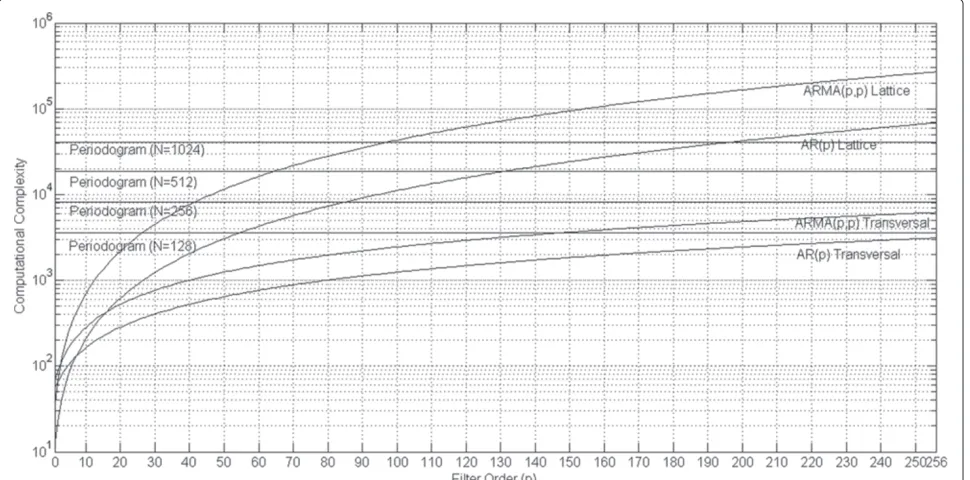
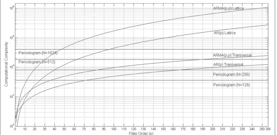
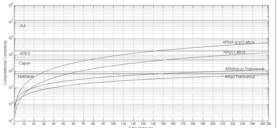
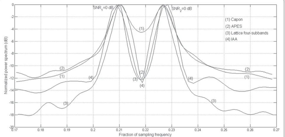
An adaptive FIR filtering approach to spectral esti-mation, which is referred to as amplitude and phase estimation of a sinusoid (APES) and has applications to radar target recognition, was proposed by Li and Sto-ica [40], and the adaptive FIR filtering approach to the Capon method was also discussed by Stoica and Moses [41]. Moreover, the APES method has been extended to array processing by Yardibi et al. [42], and named as iterative adaptive approach for amplitude and phase esti-mation (IAA-APES). An FIR filtering reinterpretation of the Thomson’s multitaper method [43,44] with applica-tions to spectrum sensing for cognitive radio was also presented by Farhang-Boroujeny [45]. Recently, compu-tationally efficient versions of the adaptive Capon and APES, and IAA methods have been proposed in [46,47], respectively. In this article, we compare the complexity and performance of our method with those of the Peri-odogram, multitaper, Capon, APES, and IAA methods,
and show that our method is competitive in terms of complexity and performance.
The remainder of this article is organized as follows. In Section 2, we present the development of the new multi-channel ARMA lattice prediction filter using the modified SPMLSs. In Section 3, we develop the new Levinson– Durbin type multichannel conversion algorithm for the modified SPMLSs, and relate lattice parameters to process parameters. Spectrum estimation expression in two-subbands is given in Section 4. The computational com-plexity computations are treated in Section 5. Section 6 is concerned with the experimental results. Finally, Section 7 is about the discussions of results and conclusions. The following notations are used in this article. (•)∗represents the complex conjugate of (•). (•)T and (•)H stand for the transpose and the Hermitian transpose of (•), respectively. The variablesm,i, andnare global while all other variables are local. The variable m represents the stage number whilenandiare the time indexes related to data and coef-ficients, respectively, till we equate them in Section 3 to have a single time index.
2 Adaptive multichannel ARMA lattice prediction filtering
2.1 Multichannel prediction problem
An illustration of the adaptive multichannel ARMA pre-diction filtering in subbands for two-subband case is presented in Figure 1. Therein,y(n)represents the input fullband signal whiley1(n)andy2(n) stand for the input
subband signals. In adaptive multichannel ARMA pre-diction filtering, the objective is to find an exponentially windowed, LS solution for the AR and MA coefficients of thekth forward prediction filter that minimizes each of the two cost functions
Jk(i)= i
n=0
λi−n|fk pk(n)|
2 (2)
at each time instanti, andk=1, 2. The forward prediction errorfpkk(n)in this expression is defined as
fpkk(n)=dk(n)− ˆdik(n) (3)
and thekth forward prediction filter output,dˆki(n), is an estimate of thekth desired signal,dk(n) =yk(n), is given by
ˆ dik(n)=
pk
j=1 ˜
ak1,∗j(i)yk(n−j)+ qk
l=0 ˜
a2,k∗l(i)uˆk(n−l). (4)
Figure 1A block diagram of the adaptive multichannel ARMA prediction filtering in subbands.
obtained by delaying and feeding back thepkth-order for-ward prediction error,uˆk(n)=fpkk(n−1). Hence, the input vector to thekth ARMA filter at time instantn,y˜k(n), and the corresponding coefficient vectora˜k(i), at time instant i, are defined as
˜
yk(n)=
yk(n−1),. . .,yk(n−pk),uˆk(n),uˆk(n−1),. . ., ˆ
uk(n−qk) T
(5)
and
˜
akT(i)=a˜k
1,1(i),. . .,a˜k1,pk(i),a˜ k
2,0(i),a˜k2,1(i),. . .,a˜k2,qk(i)
,
(6)
respectively. Herein,a˜k1,j(i)anda˜k2,j(i), respectively, repre-sent thejth coefficient related to the AR and MA parts of the forward prediction filter for thekth subband at time instant i. It is assumed, without loss of generality, that pk ≥ qk. pk = qk case corresponds to the prediction filter for an ARMA(pk,pk) process, while pk > qk pre-diction filter is for a general ARMA(pk,qk) process. Note that an ARMA backward prediction can be performed for the desired signal,dk(n)=yk(n−pk), and the prediction filter in that case would use the reversed and conjugated forward prediction filter coefficients, which are defined in the backward prediction error coefficient vector as
˜
ckT(i)=˜ck
1,pk(i),. . .,c˜ k
1,1(i),c˜k2,qk(i),. . .,c˜ k
2,1(i),˜ck2,0(i)
(7)
wherec˜k1,j(i)andc˜k2,j(i)are, respectively, defined as thejth coefficient related to the AR and MA parts of the back-ward prediction filter for thekth subband at time instant i.
Consequently, the main concern of the exponentially weighted LS problem under consideration is to find, at
each timei, thekth optimal coefficient vector,a˜k(i)that would minimize the cost function
Jk(i)= i
n=0
λi−n|dk(n)− ˜akH(i)y˜
k(n)|2. (8)
The kth optimal coefficient vector related to the kth subband filter
˜
ak
opt(i)=R−k1(i)Pk(i) (9) is found by differentiatingJk(i)with respect toa˜k(i), set-ting the derivative to zero, and solving for a˜k(i), where
Rk(i)= i
n=0 λi−ny˜
k(n)y˜Hk(n) (10) and
Pk(i)= i
n=0 λi−ny˜
k(n)dk∗(n). (11)
2.2 Sequential lattice orthogonalization
In order to find a modular, regular, and simple solution to the two-subband ARMA prediction problem, we would like to use a single multichannel lattice filter as depicted in Figure 2, instead of using two separate transversal fil-ters and solving two separate optimization problems as in Figure 1. We would also like to avoid direct evalua-tions as in (9), and achieve good numerical properties. As the number of channels at different sections of the proposed multichannel lattice filter is different due to the sequential processing nature of SPMLSs, we carry out the exponentially weightedLSoptimization problem by taking into consideration each of these sections sepa-rately, and therefore we assume that the filter is comprised of three cascaded filters, which are two-channel, three-channel, and four-channel lattice sections; and we use a different index for each section while usingmto indicate a stage in the whole filter. We also assumep1=p2for the
Figure 2A block diagram of the adaptive multichannel ARMA lattice prediction filtering in subbands.
In order to sequentially solve the exponentially weighted LS optimization problem under consideration, we first organize the elements of input signal vectors y1(n) =
[y1(n),. . .,y1(n−)]T, and y2(n)=[y2(n),. . .,y2(n−)]T
according to the natural ordering of SPMLSs as
¯
y+1(n)=
⎡ ⎢ ⎢ ⎢ ⎢ ⎢ ⎢ ⎢ ⎢ ⎣
y1(n)
y2(n)
y1(n−1)
y2(n−1) − − −− y1(n−)
y2(n−)
⎤ ⎥ ⎥ ⎥ ⎥ ⎥ ⎥ ⎥ ⎥ ⎦ (12)
and input to two-channel stages for which the stage num-ber (m) has a range of values given by 0<m≤(p1−q1).
Accordingly, we redefine Equations (10) and (11) using this new data vector as follows
R(i)= i
n=0 λi−ny¯
+1(n)y¯H+1(n) (13)
and
P,k(i)= i
n=0 λi−ny¯
+1(n)dk∗(n) (14)
where k = 1, 2. The orthogonalization of data using SPMLSs corresponds to the transformation of (13) and (14) into
Df +1(i)=
i
n=0 λi−nf
(i)y¯+1(n)y¯H+1(n)
f H
(i) (15)
and
Zf
+1,k(i)= i
n=0 λi−nf
(i−1)y¯+1(n−1)dk∗(n), (16)
respectively. Here, f(i) is the 2× 2 lower triangu-lar transformation matrix for forward prediction, and is sequentially realized stage-by-stage using 2 × 2 lower triangular transformation matrices
Lf (i)=
1 0
ˆ κf
(i−1) 1
(17)
whose diagonal elements are all equal to unity at time instant i, and κˆf(i) is the reflection coefficient com-puted at the single circular cell in the triangular-shaped self-orthogonalization processor of theth two-channel SPMLS. Then, the forward lattice predictor coefficients are computed using
f
,k(i)=D −f
+1(i−1)Z
f
+1,k(i) (18)
wheref,
k(i)represents thekth row of the 2×2lattice forward prediction reflection coefficient matrix f(i), and is also sequentially implemented stage-by-stage by means of 2×2 forward prediction reflection coefficient matrices
f (i)=
¯ κf
,1,1(i) κ¯ f ,1,2(i) ¯
κf ,2,1(i) κ¯
f ,2,2(i)
(19)
in whichκ¯f,
k,j(i)is thejth reflection coefficient related to the forward prediction of thekth channel signal, and it is computed at the(k,j)th single circular cell of the square-shaped reference-orthogonalization processor related to forward prediction at theth two-channel SPMLS. Note that the matrix inversion operation in Equation (9) is transformed into a simple scalar inversion operation in (18) due to the diagonal nature ofDf+1(i). The backward prediction counterpart of this optimization problem is similarly solved using 2×2 lower triangular transforma-tion matricesLb(i), and 2×2 lattice backward prediction reflection coefficient matrices,b(i).
After the processing of input signals by two-channel lattice stages, the delayed and fed back forward predic-tion error uˆ1(n) = fp1(n − 1) is incorporated at the (p1−q1+1)thstage, as the third channel. Accordingly, we
expand the optimization problem by organizing the ele-ments of the input data vectorsy1(n)=[y1(n),. . .,y1(n− α)]T , y2(n) =[y2(n),. . .,y2(n − α)]T, and uˆ1(n) = [uˆ1(n),. . .,uˆ1(n−α)]Tas follows:
¯
yα+1(n)=
⎡ ⎢ ⎢ ⎢ ⎢ ⎢ ⎢ ⎢ ⎢ ⎣
y1(n)
y2(n) ˆ u1(n) − − −− y1(n−α)
y2(n−α) ˆ
u1(n−α)
and input to three-channel lattice section, where the stage number (m) takes values in the range given by(p1−q1) <m≤ (p2−q2). Subsequently, we solve the optimization problem in (18) once again with the new input vector, in which case
f
α(i)andfα(i)are the 3α×3αlower triangular transformation and the 3×3αforward lattice prediction coefficient matrices, respectively.fα(i)is computed sequentially by means of 3×3 lower triangular transformation matrices,Lfα(i), andfα(i)is similarly realized stage-by-stage making use of 3×3 forward prediction coefficient matrices,fα(i), at time instanti. Note that, since the delayed and fed back signal is considered to constitute a new channel in the multichannel sequential lattice filtering, we have three desired signals at this point,dk(n), wherek=1, 2, 3, one of which did not exist in the optimization problem stated in Section 2.1, and this new desired signal,d3(n), is related to the MA part of the first subband ARMA modeling.
Finally, the optimization problem is expanded one more time with the inclusion of the second delayed and fed back forward prediction erroruˆ2(n)=fp2(n−1), and this time, the elements of input data vectors y1(n)=[y1(n),. . .,y1(n− ν)]T,y2(n)=[y2(n),. . .,y2(n−ν)]T,uˆ1(n)=[uˆ1(n),. . .,uˆ1(n−ν)]T, anduˆ2(n)=[uˆ2(n),. . .,uˆ2(n−ν)]T are organized
as
¯
yν+1(n)= ⎡ ⎢ ⎢ ⎢ ⎢ ⎢ ⎢ ⎢ ⎢ ⎢ ⎢ ⎢ ⎢ ⎣
y1(n) y2(n) ˆ u1(n) ˆ u2(n) − − −− y1(n−ν) y2(n−ν) ˆ u1(n−ν) ˆ u2(n−ν)
⎤ ⎥ ⎥ ⎥ ⎥ ⎥ ⎥ ⎥ ⎥ ⎥ ⎥ ⎥ ⎥ ⎦
(21)
where the stage number (m) is in the range given by(p2−q2) < m≤ p2due to four-channel processing. Similar to
two-channel and three-channel cases, we solve the optimization problem in (18) using the new data vector in Equation (21), in which casefν(i)andfν(i)are 4ν×4νlower triangular transformation, and 4×4νforward lattice prediction coefficient matrices at the time instant i, respectively. Similar to previous cases, these matrices are computed stage-by-stage by the use of 4×4 lower triangular transformation matrices,Lfν(i), and 4×4 forward prediction coefficient matrices,fν(i), at time instanti, respectively. As the second delayed and fed back signal is also considered as a new channel in the multichannel sequential lattice filtering, hereafter we have four desired signals,dk(n), wherek=1, 2, 3, 4, and this fourth desired signal,d4(n), is associated with the MA part of the second subband ARMA modeling.
2.3 Matrix visualization
In order to further explain the sequential lattice orthogonalization, we consider a(8, 5)and(8, 2)ARMA prediction lattice prediction filter for the first and second subbands, and organize the elements of input data vectors y1(n) =
[y1(n),. . .,y1(n−8)]T, y2(n) = [y2(n),. . .,y2(n−8)]T, uˆ1(n) = [uˆ1(n),uˆ1(n−1),. . .,uˆ1(n−5)]T, anduˆ2(n) =
[uˆ2(n),uˆ2(n−1),. . .,uˆ2(n−2)]Tas columns of a matrix,
⎡ ⎢ ⎢ ⎣
y1(n) y1(n−1) y1(n−2) y1(n−3) y1(n−4) y1(n−5) y1(n−6) y1(n−7) y1(n−8) y2(n) y2(n−1) y1(n−2) y1(n−3) y2(n−4) y2(n−5) y2(n−6) y2(n−7) y2(n−8)
ˆ
u1(n) uˆ1(n−1) uˆ1(n−2) uˆ1(n−3) uˆ1(n−4) uˆ1(n−5) ˆ
u2(n) uˆ2(n−1) uˆ2(n−2) ⎤ ⎥ ⎥
⎦ (22)
RASIP
Jo
ur
nal
o
n
A
dv
anc
es
in
Si
gnal
Pr
oc
essi
ng
2013,
2013
:9
P
a
g
e
7
o
f
3
6
e
u
rasi
p
jo
u
rnal
s.c
o
m
/co
ntent/2013/1/9
ˆ dki(n) =
p1−q1
m=1 2
j=1 ¯ κf∗
m,k,j(i−1)bˆ j
m−1(n−1)
+ p2−q2
m=p1−q1+1
3
j=1 ¯ κf∗
m,k,j(i−1)bˆ j
m−1(n−1)
+ p2
m=p2−q2+1
4
j=1 ¯
κmf∗,k,j(i−1)bˆjm−1(n−1). (23)
Here, the first and second summations represent the prediction accomplished by the two-channel and three-channel sections, respectively, and the fourth summation is connected with the four-channel prediction section. In each section,κ¯mf,k,j(i) represents the jth forward pre-diction reflection coefficient at the mth stage related to the kth channel as defined in the previous sub-section, and bˆjm−1(n) represents the jth element of the self-orthogonalized backward prediction error sig-nal vector, bˆm−1(n), at the input of the mth stage.
The self-orthogonalized backward prediction error vector, ˆ
bm−1(n), is produced by the lower triangular
transfor-mation of the input backward prediction error vector,
bm−1(n), usingLfm(n), and this operation is accomplished at the triangular shaped self-orthogonalization processor (related to forward prediction) of themth SPMLS. Note that the sizes of vectors, bˆm−1(n), bm−1(n), and matrix,
Lf
m(n), at different sections of the proposed lattice filter are as follows: 2×1, and 2×2 in two-channel section, 3×1, and 3×3 in three-channel section, and 4×1, and 4×4 in four-channel section, respectively.
We would also like to point out that a lattice filter for fullband ARMA spectrum estimation is a special form of the two-subband implementation, and therefore it can similarly be realized using sequential processing one-channel and two-one-channel lattice stages as illustrated in Figure 4 for an ARMA(10,2) implementation.
3 Conversion of lattice coefficients to process parameters
Since the mathematical link between process parameters and reflection coefficients of a lattice prediction filter is provided by the Levinson–Durbin algorithm [48,49], we develop a new Levinson–Durbin type conversion algo-rithm specifically for SPMLSs in order to convert lat-tice reflection coefficients to subband ARMA process parameters. Due to the sequential nature of the pro-posed lattice structure, we carry out the development of the new Levinson–Durbin type multichannel conver-sion algorithm by taking into consideration each of these sections separately, and therefore we assume that the filter is comprised of three cascaded filters as in Section 2.2.
We first consider the conversion algorithm for the two-channel section of lattice prediction filter, and we organize the input signal samples to two-channel lattices as
¯
y+1(n)= ⎡ ⎢ ⎢ ⎢ ⎢ ⎢ ⎢ ⎢ ⎢ ⎣ ⎡
⎣− − −−y1(n) y1(n−)
⎤ ⎦
⎡
⎣− − −−y2(n) y2(n−)
⎤ ⎦ ⎤ ⎥ ⎥ ⎥ ⎥ ⎥ ⎥ ⎥ ⎥ ⎦ = ⎡ ⎢ ⎢ ⎢ ⎢ ⎢ ⎢ ⎢ ⎢ ⎣ ⎡
⎣ − − −−y1(n) y1(n−1)
⎤ ⎦
⎡
⎣ − − −−y2(n) y2(n−1)
⎤ ⎦ ⎤ ⎥ ⎥ ⎥ ⎥ ⎥ ⎥ ⎥ ⎥ ⎦ (24)
where we define the data vectors as y1(n) =
[y1(n),. . .,y1(n−+1)]T ,y2(n) = [y2(n),. . .,y2(n− +1)]T, and 0<m≤(p1−q1). The corresponding
for-ward and backfor-ward prediction error coefficient matrices for theth-order transversal filter for thekth channel are defined as
ˆ
akT(i)= aˆk
0(i),aˆk1(i),aˆk2(i),. . .,. . .,aˆk2−2(i),aˆk2−1(i),aˆk2(i)
(25)
and
ˆ
ckT(i)= ˆck
2(i),ˆck2−1(i),ˆck2−2(i),. . .,. . .,ˆck2(i),cˆk1(i),cˆk0(i)
(26)
where k = 1, 2 due to two-channel lattice processing, and aˆk0(i) = ˆck0(i) = 1.0. Since the signal time shift-ing and ordershift-ing properties of SPMLSs when expressed in matrix form as in Equation (12) are different than the organization of input signal samples in matrix form as in Equation (24), we use (2+ 1) × (2+ 1) shuf-fling matrices, J1+1 for the first channel and J2+1 for the second channel, to reorder the elements of coeffi-cient matrices,aˆ1H(i),aˆ2H(i)andcˆ1H(i),cˆ2H(i), according to the sample ordering of SPMLSs. Therefore, the for-ward and backfor-ward prediction errors for the end of the observation interval n = i at the output of the gen-eral th-order filters with transversal structure can be stated as
f1(n) f2(n)
=
J1
+1aˆ1H(n) 0
0 J2
+1aˆ2H(n)
¯
y+1(n) (27)
b1(n) b2(n)
=
J1
+1cˆ1H(n) 0
0 J2
+1cˆ2H(n)
¯
Figure 4A diagram of the two-channel ARMA lattice filter structure for fullband spectrum estimation.
where0is a 1x(+1)zero matrix. Then, we can express the(−1)th prediction errors as
f1−1(n) f2−1(n) = J1 +1 ˆ a1H
−1(n) 0 0
0
0 J2
+1
ˆ a2H
−1(n) 0 0
y¯+1(n)
(29)
b1−1(n−1) b2−1(n−1)
= J1 +1
0 0 cˆ1H−1(n−1) 0
0 J2
+1
0 0 cˆ2H−1(n−1)
¯ y+1(n)
(30)
Note that the size of each coefficient matrix increases by two when the order of prediction filter increases from−1 to, and0is a 1×(+1)zero matrix as before. Subse-quently, we define theth-order prediction errors in terms of lattice parameters and the(−1)th-order prediction errors as follows
f1
(n) f2(n)
=
f1−1(n) f2−1(n)
+
¯ κf∗
,1,1(n−1) κ¯
f∗ ,1,2(n−1) ¯
κf∗
,2,1(n−1) κ¯
f∗ ,2,2(n−1)
×
1 0
ˆ κf∗
(n−2) 1
b1−1(n−1) b2−1(n−1)
(31)
b1(n) b2(n)
=
b1
−1(n−1) b2−1(n−1)
+
¯ κb∗
,1,1(n−1) κ¯
b∗ ,1,2(n−1) ¯
κb∗
,2,1(n−1) κ¯
b∗ ,2,2(n−1)
×
1 0
ˆ κb∗
(n−1) 1
f1−1(n) f2−1(n)
(32)
where the lower coefficient triangular and square matrices are generated in triangular shaped self-orthogonalization and square shaped reference-orthogonalization proces-sors in a two-channel SPMLS as defined in Equations (17) and (19). Accordingly, we multiply these lower triangular and square coefficient matrices, and make the following definitions
f (n)=
f
,1,1(n) f ,1,2(n) f
,2,1(n) f ,2,2(n)
=
¯ κf
,1,1(n)+ ¯κ f ,1,2(n)κˆ
f
(n−1) κ¯f,1,2(n) ¯
κf
,2,1(n)+ ¯κ f ,2,2(n)κˆ
f
(n−1) κ¯f,2,2(n)
(33)
b (n)=
b
,1,1(n) b ,1,2(n) b
,2,1(n) b ,2,2(n)
=
¯ κb
,1,1(n)+ ¯κ b ,1,2(n)κˆ
b
(n) κ¯b,1,2(n) ¯
κb
,2,1(n)+ ¯κ b ,2,2(n)κˆ
b
(n) κ¯b,2,2(n)
(34)
in order to obtain compact versions of Equations (31) and (32) as follows
f1(n) f2(n)
=
f1−1(n) f2−1(n)
+f∗ (n−1)
b1−1(n−1) b2−1(n−1)
b1(n) b2(n)
=
b1−1(n−1) b2−1(n−1)
+b∗ (n−1)
f1−1(n) f2−1(n)
.
(36)
Then, the th-order prediction error matrices in Equations (27) and (28), and the(−1)th-order prediction error matrices in Equations (29) and (30) are substituted in theth-order prediction error expressions in (35) and (36) so as to obtain the following pairs of order updates
ˆ
a1
(n)=
ˆ
a1
−1(n)
0
+f∗
,1,1(n−1)J
1 +1 0 ˆ c1
−1(n−1)
+f∗,1,2(n−1)J
2 +1 0 ˆ c2
−1(n−1)
(37)
ˆ
a2
(n)=
ˆ
a2
−1(n)
0
+f∗
,2,1(n−1)J
1 +1 0 ˆ c1
−1(n−1)
+f∗
,2,2(n−1)J
2 +1 0 ˆ c2
−1(n−1)
(38)
ˆ
c1
(n)=
0
ˆ
c1
−1(n−1)
+b∗
,1,1(n−1)J 1 +1
ˆ
a1
−1(n)
0
+b∗
,1,2(n−1)J
2
+1
ˆ
a2
−1(n)
0
(39)
ˆ
c2
(n)=
0
ˆ
c2
−1(n−1)
+b∗
,2,1(n−1)J 1 +1
ˆ
a1
−1(n)
0
+b∗
,2,2(n−1)J
2
+1
ˆ
a2
−1(n)
0
(40)
and since the size of each coefficient matrix increase by two,0is a 2×1 zero matrix. The three-channel section starts with the incorporation of the third channel (uˆ1(n))
as the new channel at the(p1−q1+1)th stage. In order to
develop the Levinson–Durbin algorithm for this section, we assume that three-channel section is a separate filter, and thereby considering the input signal samples to the three-channel section as follows
¯
yα+1(n)= ⎡ ⎢ ⎢ ⎢ ⎢ ⎢ ⎢ ⎢ ⎢ ⎢ ⎢ ⎢ ⎢ ⎢ ⎢ ⎢ ⎢ ⎣ ⎡
⎣ − − −−y1(n) y1(n−α)
⎤ ⎦
⎡
⎣ − − −−y2(n) y2(n−α)
⎤ ⎦
⎡
⎣ − − −−u1ˆ (n)
ˆ u1(n−α)
⎤ ⎦ ⎤ ⎥ ⎥ ⎥ ⎥ ⎥ ⎥ ⎥ ⎥ ⎥ ⎥ ⎥ ⎥ ⎥ ⎥ ⎥ ⎥ ⎦ = ⎡ ⎢ ⎢ ⎢ ⎢ ⎢ ⎢ ⎢ ⎢ ⎢ ⎢ ⎢ ⎢ ⎢ ⎢ ⎢ ⎢ ⎣ ⎡
⎣− − −−y1(n) y1(n−1)
⎤ ⎦
⎡
⎣− − −−y2(n) y2(n−1)
⎤ ⎦
⎡
⎣ − − −−uˆ1(n)
ˆ u1(n−1)
⎤ ⎦ ⎤ ⎥ ⎥ ⎥ ⎥ ⎥ ⎥ ⎥ ⎥ ⎥ ⎥ ⎥ ⎥ ⎥ ⎥ ⎥ ⎥ ⎦ (41)
where y1(n) =
y1(n),. . .,y1(n−α+1)
T
, y2(n) =
y2(n),. . .,y2(n−α+1)T, and uˆ1(n) = uˆ1(n),. . ., ˆ
u1(n−α+1)
T
. Correspondingly, the forward and back-ward prediction error coefficient matrices for the α th-order transversal filtering are defined as
ˆ
akT(n)=aˆk
0(n),aˆk1(n),aˆ2k(n),aˆ3k(n),. . .,. . .,
ˆ
ak3α−2(n),aˆk3α−1(n),aˆk3α(n)
(42)
and ˆ
ckT(n)=ˆck
3α(n),cˆk3α−1(n),ˆck3α−2(n),. . .,. . .,
ˆ
ck3(n),ˆck2(n),ˆck1(n),cˆk0(n)
(43)
wherek = 1, 2, 3 due to three-channel processing. Then, the prediction filtering continues with three-channel lat-tice stages for(p1−q1) <m≤(p2−q2). The Levinson–
Durbin recursions for the three-channel section can be developed similar to the two-channel section by estab-lishing the mathematical link between transversal and lattice filter coefficients. Since the organization of signal samples in Equation (41) is different than the ordering of signal samples entering into three-channel SPMLSs in (20), we use (3α + 1) × (3α + 1) shuffling matrices,
J1
α+1 for the first channel, J2α+1 for the second
chan-nel, and J3α+1 for the third channel to reorder the ele-ments of coefficient matrices,aˆ1αH(n),aˆα2H(n),aˆ3αH(n)and ˆ
c1H
α (n),cˆ2αH(n),cˆ3αH(n), according to the sample ordering of SPMLSs. Similar to Equations (27) and (28) in two-channel case, the forward and backward prediction errors in three-channel case for the output of the general α th-order filter with transversal structure are expressed as
⎡ ⎣f
1
α(n) fα2(n) f3
α(n)
⎤
⎦=
⎡ ⎣J
1
α+1aˆ1αH(n) 0 0
0 J2
α+1aˆ2αH(n) 0
0 0 J3
α+1aˆ3αH(n) ⎤ ⎦y¯α+1(n)
(44)
⎡ ⎣b
1
α(n) b2α(n) b3
α(n)
⎤
⎦=
⎡ ⎣J
1
α+1cˆ1αH(n) 0 0
0 J2
α+1cˆ2αH(n) 0
0 0 J3
α+1cˆ3αH(n) ⎤ ⎦y¯α+1(n)
⎡ ⎣f
1
α−1(n) fα2−1(n) f3
α−1(n) ⎤
⎦=
⎡ ⎣J
1
α+1
ˆ a1H
α−1(n) 0 0 0
0 0
0 J2
α+1
ˆ a2H
α−1(n) 0 0 0
0
0 0 J3
α+1
ˆ a3H
α−1(n) 0 0 0
⎤
⎦y¯α+1(n) (46)
⎡ ⎣b
1
α−1(n−1) b2α−1(n−1) b3α−1(n−1)
⎤
⎦=
⎡ ⎣J
1
α+1
0 0 0 cˆ1H
α−1(n−1)
0 0
0 J2
α+1
0 0 0 cˆ2H
α−1(n−1)
0
0 0 J3
α+1
0 0 0 cˆ3αH−1(n−1)
⎤
⎦y¯α+1(n). (47)
Note that the size of each coefficient matrix in three-channel case increases by three when the order of predic-tion filter increases fromα−1 toα. Similar to Equations (35) and (36) in two-channel case, the lattice prediction errors for theαththree-channel stage can be expressed in compact form with the following equations
⎡ ⎣f
1
α(n) fα2(n) fα3(n)
⎤
⎦=
⎡ ⎣f
1
α−1(n)
fα2−1(n) fα3−1(n)
⎤ ⎦+f∗
α (n−1) ⎡ ⎣b
1
α−1(n−1)
b2α−1(n−1) b3α−1(n−1)
⎤ ⎦ (48) ⎡ ⎣b 1
α(n) b2α(n) b2α(n)
⎤
⎦=
⎡ ⎣b
1
α−1(n−1)
b2α−1(n−1) b3α−1(n−1)
⎤ ⎦+b∗
α (n−1) ⎡ ⎣f
1
α−1(n)
fα2−1(n) fα3−1(n)
⎤ ⎦
(49)
where
f α(n)=
⎡ ⎢ ⎣
f
α,1,1(n) f
α,1,2(n) f α,1,3(n) f
α,2,1(n) f
α,2,2(n) f α,2,3(n) f
α,3,1(n) f
α,3,2(n) f α,3,3(n)
⎤ ⎥ ⎦ = ⎡ ⎢ ⎣ ¯ κf
α,1,1(n) κ¯ f α,1,2(n) κ¯
f α,1,3(n) ¯
κf α,2,1(n) κ¯
f α,2,2(n) κ¯
f α,2,3(n) ¯
κf α,3,1(n) κ¯
f α,3,2(n) κ¯
f α,3,3(n)
⎤ ⎥ ⎦ × ⎡ ⎢ ⎣
1 0 0
ˆ κf
α,2,1(n−1) 1 0
ˆ κf
α,3,1(n−1) κˆ f
α,3,2(n−1) 1 ⎤ ⎥ ⎦
and
b α(n)=
⎡ ⎢ ⎣
b
α,1,1(n) αb,1,2(n) αb,1,3(n) b
α,2,1(n) αb,2,2(n) αb,2,3(n) b
α,3,1(n) αb,3,2(n) αb,3,3(n) ⎤ ⎥ ⎦ = ⎡ ⎢ ⎣ ¯ κb
α,1,1(n) κ¯ b α,1,2(n) κ¯
b α,1,3(n) ¯
κb α,2,1(n) κ¯
b α,2,2(n) κ¯
b α,2,3(n) ¯
κb α,3,1(n) κ¯
b α,3,2(n) κ¯
b α,3,3(n)
⎤ ⎥ ⎦
×
⎡
⎣κˆb 1 0 0
α,2,1(n) 1 0 ˆ
κb
α,3,1(n) κˆαb,3,2(n) 1 ⎤ ⎦.
The αth-order prediction error matrices in Equations (44) and (45), and the (α−1)th-order prediction error matrices in Equations (46) and (47) are subsequently sub-stituted in theαth-order prediction error expressions in (48) and (49) so that the following pairs of order updates are produced
ˆ
a1
α(n)=
ˆ
a1
α−1(n)
0
+f∗
α,1,1(n−1)J1α+1
0
ˆ
c1
α−1(n−1)
+. . .+f∗
α,1,3(n−1)J3α+1
0
ˆ
c3
α−1(n−1)
(50)
ˆ
a2
α(n)=
ˆ
a2
α−1(n)
0
+f∗
α,2,1(n−1)J
1
α+1
0
ˆ
c1
α−1(n−1)
+. . .+f∗
α,2,3(n−1)J
3
α+1
0
ˆ
c3
α−1(n−1)
(51)
ˆ
a3
α(n)=
ˆ
a3
α−1(n)
0
+f∗
α,3,1(n−1)J
1
α+1
0
ˆ
c1
α−1(n−1)
+. . .+f∗
α,3,3(n−1)J
3
α+1
0
ˆ
c3
α−1(n−1)
(52)
ˆ
c1
α(n)=
0
ˆ
c1
α−1(n−1)
+b∗
α,1,1(n−1)J
1
α+1
ˆ
a1
α−1(n)
0
+. . .+b∗
α,1,3(n−1)J
3
α+1
ˆ
a3
α−1(n)
0
(53)
ˆ
c2
α(n)=
0
ˆ
c2
α−1(n−1)
+b∗
α,2,1(n−1)J
1
α+1
ˆ
a1
α−1(n)
0
+. . .+b∗
α,2,3(n−1)J
3
α+1
ˆ
a3
α−1(n)
0
(54)
ˆ
c3
α(n)=
0
ˆ
c3
α−1(n−1)
+b∗
α,3,1(n−1)J
1
α+1
ˆ
a1
α−1(n)
0
+. . .+b∗
α,3,3(n−1)J
3
α+1
ˆ
a3
α−1(n)
0
where the size of0 is a 3 × 1 zero matrix. Finally, the fourth channel(uˆ2(n)), which represents the fed back and
delayed signal related to the second subband, is taken into the orthogonalization process at the(p2−q2+1)th stage,
and the prediction filtering continues with four-channel lattice stages through(p2−q2) < m ≤ p2. In order to
develop the Levinson–Durbin recursions for this section, we define the forward and backward prediction error coefficient matrices for theνth-order transversal filtering as
ˆ
akT(n)=aˆk
0(n),aˆk1(n),aˆk2(n),aˆk3(n),aˆk4(n),. . .,. . ., ˆ
a4kν−3(n),aˆk4ν−2(n),aˆk4ν−1(n),aˆk4ν(n)
(56)
and
ˆ
ckT(n)=ˆck
4ν(n),ˆck4ν−1(n),cˆk4ν−2(n),cˆk4ν−3(n),. . .,. . ., ˆ
ck4(n),cˆk3(n),cˆk2(n),cˆk1(n),ˆck0(n)
(57)
where k = 1, 2, 3, 4 due to four-channel lattice process-ing, and we also visualize as before that the following organization of the elements of input vectors y1(n) =
[y1(n),. . .,y1(n−ν+1)]T,y2(n)=[y2(n),. . .,y2(n−ν+
1)]T,uˆ1(n) =[uˆ1(n),. . .,uˆ1(n−ν+1)]T, and uˆ2(n) = [uˆ2(n),. . .,uˆ2(n−ν+1)]Tis established:
¯
yν+1(n)=
⎡ ⎢ ⎢ ⎢ ⎢ ⎢ ⎢ ⎢ ⎢ ⎢ ⎢ ⎢ ⎢ ⎢ ⎢ ⎢ ⎢ ⎢ ⎢ ⎢ ⎢ ⎢ ⎢ ⎢ ⎢ ⎣ ⎡
⎣− − −−y1(n) y1(n−ν)
⎤ ⎦
⎡
⎣− − −−y2(n) y2(n−ν)
⎤ ⎦
⎡
⎣ − − −−uˆ1(n)
ˆ
u1(n−ν)
⎤ ⎦
⎡
⎣ − − −−uˆ2(n)
ˆ
u2(n−ν)
⎤ ⎦ ⎤ ⎥ ⎥ ⎥ ⎥ ⎥ ⎥ ⎥ ⎥ ⎥ ⎥ ⎥ ⎥ ⎥ ⎥ ⎥ ⎥ ⎥ ⎥ ⎥ ⎥ ⎥ ⎥ ⎥ ⎥ ⎦ = ⎡ ⎢ ⎢ ⎢ ⎢ ⎢ ⎢ ⎢ ⎢ ⎢ ⎢ ⎢ ⎢ ⎢ ⎢ ⎢ ⎢ ⎢ ⎢ ⎢ ⎢ ⎢ ⎢ ⎢ ⎢ ⎣ ⎡
⎣ − − −−y1(n)
y1(n−1)
⎤ ⎦
⎡
⎣− − −−y2(n)
y2(n−1)
⎤ ⎦
⎡
⎣ − − −−uˆ1(n)
ˆ
u1(n−1)
⎤ ⎦
⎡
⎣ − − −−uˆ2(n)
ˆ
u2(n−1)
⎤ ⎦ ⎤ ⎥ ⎥ ⎥ ⎥ ⎥ ⎥ ⎥ ⎥ ⎥ ⎥ ⎥ ⎥ ⎥ ⎥ ⎥ ⎥ ⎥ ⎥ ⎥ ⎥ ⎥ ⎥ ⎥ ⎥ ⎦ . (58)
Similar to the previous two steps, the signal sample ordering in Equation (58) is different than the order-ing in Equation (21), hence we use (4ν + 1) × (4ν + 1) shuffling matrices, J1ν+1 for the first channel, J2ν+1 for the second channel, J3ν+1 for the third channel, and
J4
ν+1 for the fourth channel to reorder the elements
of coefficient matricesaˆ1H
ν (n),aˆ2νH(n),aˆν3H(n),aˆ4νH(n)and ˆ
c1H
ν (n),cˆ2νH(n),cˆν3H(n),cˆ4νH(n), according to the sample
ordering of SPMLSs. Then, the development of the Levinson–Durbin recursions for this section unfolds as in two and three-channel sections. First, theνth and the
(ν −1)th order forward and backward prediction errors are stated as the output of a transversal. Second, the pre-diction order update equations for the (ν − 1)th and the νth-orders are expressed for a four-channel lattice section, and finally theνth and the(ν−1)th-order forward and backward transversal filter prediction error expres-sions are substituted in the lattice prediction order update equations such that the following pairs of order updates are obtained
ˆ
a1
ν(n)=
ˆ
a1
ν−1(n)
0
+f∗
ν,1,1(n−1)J1ν+1
0
ˆ
c1
ν−1(n−1)
+ · · · +f∗
ν,1,4(n−1)J
4
ν+1
0
ˆ
c4
ν−1(n−1)
(59)
ˆ
a2
ν(n)=
ˆ
a2
ν−1(n)
0
+f∗
ν,2,1(n−1)J1ν+1
0
ˆ
c1
ν−1(n−1)
+ · · · +f∗
ν,2,4(n−1)J
4
ν+1
0
ˆ
c4
ν−1(n−1)
(60)
ˆ
a3
ν(n)=
ˆ
a3
ν−1(n)
0
+f∗
ν,3,1(n−1)J1ν+1
0
ˆ
c1
ν−1(n−1)
+ · · · +f∗
ν,3,4(n−1)J
4
ν+1
0
ˆ
c4
ν−1(n−1)
(61)
ˆ
a4
ν(n)=
ˆ
a4
ν−1(n)
0
+f∗
ν,4,1(n−1)J1ν+1
0
ˆ
c1
ν−1(n−1)
+ · · · +f∗
ν,4,4(n−1)J
4
ν+1
0
ˆ
c4
ν−1(n−1)
(62)
ˆ
c1
ν(n)=
0
ˆ
c1
ν−1(n−1)
+b∗
ν,1,1(n−1)J
1
ν+1
ˆ
a1
ν−1(n)
0
+ · · · +b∗
ν,1,4(n−1)J
4
ν+1
ˆ
a4
ν−1(n)
0
(63)
ˆ
c2
ν(n)=
0
ˆ
c2
ν−1(n−1)
+b∗
ν,2,1(n−1)J
1
ν+1
ˆ
a1
ν−1(n)
0
+ · · · +b∗
ν,2,4(n−1)J
4
ν+1
ˆ
a4
ν−1(n)
0
ˆ
c3
ν(n)=
0
ˆ
c3
ν−1(n−1)
+b∗
ν,3,1(n−1)J
1
ν+1
ˆ
a1
ν−1(n)
0
+ · · · +b∗
ν,3,4(n−1)J
4
ν+1
ˆ
a4
ν−1(n)
0
(65)
ˆ
c4
ν(n)=
0
ˆ
c4
ν−1(n−1)
+b∗
ν,4,1(n−1)J
1
ν+1
ˆ
a1
ν−1(n)
0
+ · · · +b∗
ν,4,4(n−1)J
4
ν+1
ˆ
a4
ν−1(n)
0
.
(66)
Note that 0 is a 4 × 1 zero matrix, and that conver-sion of lattice parameters to process parameters started with two channels, but ended with four channels due to sequential processing. The new Levinson–Durbin type conversion algorithm for a fullband ARMA spectrum estimation can be similarly developed as a special case of subband implementation. The lattice prediction filter for fullband ARMA spectrum estimation, which consists of one and two-channel sections, is shown in Figure 4. The corresponding conversion algorithm can also be real-ized in two sections as summarreal-ized in Subsection New Levinson-Durbin Type Conversion Algorithm for Two-Channel ARMA Lattice Prediction.
3.1 New Levinson-Durbin type conversion algorithm for two-channel ARMA lattice prediction
Initialization :
ˆ
a10(n)=1.0, ˆc10(n)=1.0, aˆ2p−q(n)=1.0, ˆ
c20(n)=1.0. (67)
One-channel Section(0<m≤(p−q)):
ˆ
a1
m(n)=
ˆ
a1
m−1(n)
0
+f∗ m,1(n−1)
0 ˆ
c1
m−1(n−1)
(68)
ˆ
c1
m(n)=
0 ˆ
c1
m−1(n−1)
+b∗ m,1(n−1)
ˆ
a1
m−1(n)
0
.
(69)
Two-channel Section((p−q) <m≤p):
ˆ a1
m(n)=
ˆ a1
m−1(n) 0
+f∗
m,1,1(n−1)J1m+1
0 ˆ c1
m−1(n−1)
+f∗
m,1,2(n−1)J2m+1
0 ˆ c2
m−1(n−1)
(70) ˆ a2
m(n)=
ˆ a2
m−1(n) 0
+f∗
m,2,1(n−1)J1m+1
0 ˆ c1
m−1(n−1)
+f∗
m,2,2(n−1)J2m+1
0 ˆ c2
m−1(n−1)
(71)
ˆ c1
m(n)=
0 ˆ c1
m−1(n−1)
+b∗
m,1,1(n−1)J 1 m+1
ˆ a1
m−1(n) 0
+b∗
m,1,2(n−1)J 2 m+1
ˆ a2
m−1(n) 0
(72)
ˆ c2
m(n)=
0 ˆ c2
m−1(n−1)
+b∗
m,2,1(n−1)J 1 m+1
ˆ a1
m−1(n) 0
+b∗
m,2,2(n−1)J 2 m+1
ˆ a2
m−1(n) 0
.
(73)
4 Spectrum estimation from subbands
After computing process parameters from lattice coef-ficients, we established the link between multichannel prediction and spectrum estimation. Hence, the estimated spectrum in subbands can be expressed in terms of the subband prediction filter parameters as
Sy(wk)=
1+ ¯a31e−jwk+ · · · + ¯a3 q1e
−jq1wk
1+ ¯a11e−jwk + · · · + ¯a1 p1e−jp
1wk
2
.σˆx21
+1+ ¯a 4
1e−jwk+ · · · + ¯a4q2e −jq2wk
1+ ¯a21e−jwk+ · · · + ¯a2 p2ejp2wk
2
.σˆx22
(74)
where σˆx2k represents the prediction error variance for the kth subband; and the coefficients, a¯11,. . .,a¯1p1 and ¯
a31,. . .,a¯3q1 are related to the AR and MA parts of the first subband ARMA spectrum while the coefficients ¯
a21,. . .,a¯2p2anda¯
4