An X-ray Diffraction Study of the Structure of Argon in the Dense Liquid Region

(1)

AN X-RAY DIFFRACTION STUDY OF THE STRUCTURE OF ARGON IN THE DENSE LIQUID REGION

Thesis by { t.< c:,5

Stephen C Smelser

In Partial Fulfillment of the Requirements For the Degree of

Doctor of Philosophy

California Institute of Technology Pasadena, California

(2)

ACKNOWLEOOMENTS

I wish to express my sincere appreciation to Professor C. J. Pings for his helpful guidance and his encouragement during the course of this investigation.

Special thanks go to Dr. Wallace Honeywell, who was

responsible for the design and construction of the apparatus; to Dr.

Paul Mikolaj, who documented the ~-filter data processing technique; to Dr. George Chang, who contributed to equipment modifications and the collecting of data; to George Griffith, Chic Nakawatase, and to June Gray. I would like to acknowledge conversations with Dr. Sten Samson, Dr. Ernest Henninger, Dr. George Wignall, Paul Fehder, Paul Morrison, and Joe Karnicky.

During my graduate studies, I have been the recipient of financial support from the California Institute of Technology and the National Science Foundation. The funds for this investigation were contributed by the Air Force Office of Scientific Research. Hewlett Packard Company donated counting equipment. I wish to express my appreciation for all these forms of support.

(3)

iii

ABSTRACT

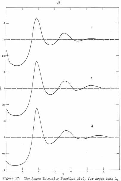
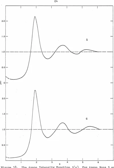
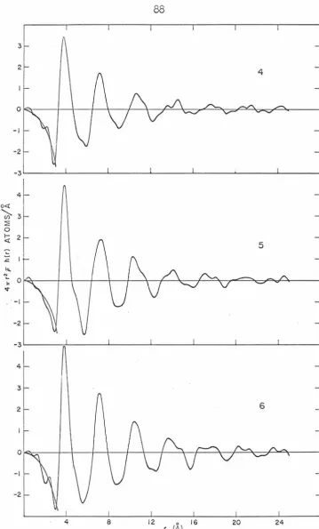
X-ray diffraction measurements were made on argon at six states in the general liquid region below the critical pressure at densities between 0.910 to 1.261 f!JI1/cc and at temperatures between lo8 to 143 °K. The intensity patterns exhibited three distinct maxima at s values of 1.91 ± .02, 3.68 ± .06 and 5.43 ± .16 ~ -l. The intensity patterns were Fourier transfonned to the net radial distribution function and the direct correlation function. The functions, 4rrr2ph(r), showed 3 maxima at low densities and 4 at the high densities at values of r of 3.85 ± 0.05, 7.29 ± .10, l0.75 ± .45

0

and 14.1 ± .5 A. A subsidiary maximum between the first and second main peaks was observed to increase in prominence and disappear

systematically as the density increased. It was not noticeably evident at either the lowest or highest density. The first zero of

0

the direct correlation function was at an r value of 3.34 ± .03 A,

0

whereas the first maximum was at 3.78 ± .06 A. Unlike previous detenninations of C(r) in this laboratory, the direct correlation

function exhibited secondary features on the shoulder of the main peak. At the highest density the direct correlation function goes negative

0

(4)

Comparisons of the direct correlation function and the radial

(5)

v

~ TITLE PAGE

I. Uncertainty Bands

43

J. Calculation of P-Y Potentials

44

IV. RESULTS

46

A.

General

46

B. Intensity Curves

47

c.

Net Radial Distribution Functions

51

D. Direct Correlation Functions

53

E. Percus-Yevick Potential Functions

54

v.

· DISCUSSION OF RESULTS

55

A.

Intensity Curves

55

B. Net Radial Distribution Functions

57

c.

Direct Correlation Functions ₅₉

D. Percus-Yevick Potential Functions

61

E. First Coordination Numbers

62

VI. CONCLUSIONS

63

REFERENCES

65

FIGURES

68

TABLES

112

APPENDICES

155

1.

THE BASIC SCATTERING EQUATION

155

2. THE BASIC DATA REDUCTION EQUATION

172

3.

DERIVATION OF THE CONFIDENCE

181

(7)

vii

~ TITLE PAGE

4.

THE BREIT-DIRAC FACTOR FOR

l85

INCOHERENT SCATTERING DETECTED BY A SCINTILLATION COUNTER

5.

THE DUAL FILTER SPECTRUM

l93

6.

CALIBRATION OF THE PRESSURE GAGE

20l

7.

THERMOMETER CALIBRATION

209

8.

CALCULATION OF ABSOR.PI'ION

220

CORRECTION FACTORS

9.

THE CORRECTION FOR HORIZONTAL

231

DIVERGENCE

PROPOSITIONS

241

1.

241

2.

255

3.

267

(8)

FIGURE

2.

4.

5.

6.

8.

10.

11.

12.

13.

LIST OF FIGURES

TITLE

Argon P, p, T Diagram Showing Locations of the Experimental States

Cross Section of Cryostat

Pictorial Illustration of the X-r~D Optical

System (Figure taken from Mikolaj1 )

Scattering Geometry used in the Argon

Experiments

Vertical Cell Alignment Data

Horizontal Cell Alignment Data

Nonnalized Cell Scattering Intensity for One

Scan (ii., ~-Filter Intensity; (!),cc-Filter

Intensity)

Normalized Cell and Sample Scattering

Intensi-ties for One Scan

(

A

,

~-Filter Intensity; ©,

a-Filter Intensity)

Comparison of Atomic Scattering fd2 , ~or Ag

Ka

Radiation. - Gingrich and Tompson ;

-Lark-Horpwitz and Miller5; fd2 Berghuis

et. ai.54 with f'

=

0.13 and f"

=

0.16 55

Comparison of Atom Scattering, fd2 , for ~oK .

Radiation. - - Eisenstein and Gingrich ;

---Ha~ris and Clayton7; fd2 Berghuis

et. ai.54 with f' = 0.18 and f"

=

0.24 55

Experimental j(s): - - Henshaw2 with Neutrons;

Gingrich and 5ompson with X-rays. Figure

taken from Rahman ,5

Experimental j (s): - - Henshaw2 - -

Estima-ted from Gingrich and

~ompson

Data6 using f d2

from Berghuis et. ai.5 with f'

=

0.13 and f"

=

0.16 55

Net Normalized Scattering Intensities (A, ~

Filter Intensity Minus a-Filter Intensity, Av?rage for Three Scans of Cell and Sample;© ~-Filter Intensity Minus a-Filter Intensity,

PAGE

68

70

71

72

73

75

77

78

(9)

FIGURE

14.

15·

16.

17.

18.

19.

20.

21.

22.

23.

ix

TITLE Argon for Five Scans of Cell)

Argon Scattering Curve for Run No. 2 with the 90% Confidence Interval, Scaled to the Total Gas Scattering Function (•, Preliminary Estimate of the Sample Intensity; O , Data;

d,

Rejected Data;=== ~ Confidence Interval; -

-Extrapolation)

The Normalized Scattering Curve for Argon Run

No. 2, before the Divergence Correction ( -Indicates the Incoherent Portion of the Total Gas Scattering Function)

Toe Argon Intensity Function, j(s), depicting the Divergence Correction for Argon Run No. 2

(o, before the Correction; after the Divergence Correction; ~ ~ ~ Extrapolation to the Compressibility Limit)

The Argon Intensity Function, j(s), for Argon Runs 1,

3

and

4

The Argon Intensity Function, j(s), for Argon Runs

5

and

6

The Effect of Temperature and Bulk Density on the Width of the Main Intensity Peak in the Argon Intensity Function, j(s) at j(s)

=

1

(Full SY!llbols, this work; Open Symbols, Mikolaj10 )

The Effect of Temperature and Bulk Density on the Height of the Main Peak in the Argon

Intensity Function, j(s) (Full Symbols, this work; Open Symbols, MikolajlO)

The Radial Atomic Density Function of Argon for Runs 1, 2 and 3 (The Parabola at small r is

4TTr2p)

The Radial Atomic Density Function of Argon for

Run~

4, 5

and

6

(The Parabola at small r is 4TTr p)

The Effect of the Divergence Correction on h(r) and C (r) ( after the Correction;

-before the Correction)

PAGE

80

81

82

83

84

86

88

(10)

FIGURE 24.

25.

26.

28.

29.

30.

31.

32.

33.

34.

35.

36.

TITLE

The Estimated Net Radial Distribution Function of Argon for Runs 1, 2 and 3

The Estimated Net Radial Distribution Function

of Argon for Runs

4, 5

and 6

The Estimated Direct Correlation Function of Argon for Runs 1, 2 and 3

The Estimated Direct Correlation Function of

Argon for Runs

4, 5

and 6

The Estimated Small r Behavior of the Direct Correlation Function of Argon for Runs 1, 3,

4,

5

and 6

The Potential Function of Liquid Argon Calcula-ted from the Percus-Yevick Equation for the Six States

The Argon Intensity Function, j(s) at p = 0.780

gm/

cc and T

=

-110°c ( - - Ver let's Function

Calculated from the P-Y Equation usinB the

Leonard-Jones Potential; o, Mikolaj 1 ). This

figure taken from Levesque and Verletl5

The Argon Intensity Function, j(s) for Run No.

2 ( - - t h i s work; o, Mikolaj and Pings11)

r0 as a Function of QCY3. (• this work; All

Others from Verlet17) "s" is the Value smax

where j(s ) is Maximum

max

The Net Radial Distribution Function of Argon

for Run No. 2. ( - - this work; • , Mikolaj

and Pingsll)

The Net Radial Distribution Function for Run

No. 2. ( - - this work; • , Wattsl9)

The Net Radial Distribution Function of Argon

for Run No. 6. ( - - this work; • , Molecular

Dynamics of Verletl7, same density but a higher temperature)

Two Dimensional Molecular Dynamics Calculation of g(r) at a Relative Packing Density of 0.5406

(from Fehder21 ), T

=

137.56°K

PAGE

91

93

95

99

100

101

(11)

FIGURE

37.

39.

40.

42.

44.

4-1.

5-1.

xi

TITLE

(from Fehder21 ), T

= 132.12

°K

(from Fehder21 ), T

=

120.74 ~K

The Direct Correlation Function of Argon Run No. 2. (--Indicates Best Estimate of Subatomic Behavior; - - Direct Results from Transform of i(s))

The Direct Correlation Function of Argon Run No. 2. ( - - this work; •, Mikolaj and Pingsl3)

The Direct Correlation Function of Argon Run No. 2. ( - - this work; e, Lennard-Jones

Potential, Percus-Yevick Approximation of Watts19)

The Direct Correlation Function of Argon (

-Run 1, this work; •, Watts1

9,

same density but

5°

higher temperature)

The Calculated Percus-Yevick Potential for Argon 2 with Error Bands vs the Lennard-Jones Potential

(o)

Depth of the Argon Potential Well as Predicted from the Percus-Yevick Equation (Open Symbols, this work; •, Mikolaj and Pings13)

First Coordination Number of Liquid Argon (Open Symbols, Calculated by Method A foli this work, All Others from Mikolaj and Pingsl • Methods A, B, C and D Described in Text)

Solid Curve Represents Coherent, Incoherent with l/B3 Recoil Correction, and Total Scattering from Helium. The Broken Curve Represents Total Scattering with No Recoil Correction. These Theoretical Curves Are According to Herzog. The Circles Indicate Experimental Values Obtained by Wollan

S-Filter and Dual Filter Spectra

PAGE 103

104

105

lo6

107

lo8

109

110

111

188

(12)

FIGURE

6-1.

6-2.

7-1.

7-2.

7-3·

8-1.

9-1.

9-2.

9-3.

9-4.

9-5·

TITLE

Schematic Diagram of the Pressure Calibration Equipment

Deviations from the Least Squares Fit (Pressure Calibration)

Schematic of Temperature Calibration Apparatus Wiring Diagram (Thermometer Calibration)

Deviation from Least Squares Fit (Thermometer Calibration)

Cell, Sample and Beam Geometry (For Absorption Factor Program)

Three Limiting Cases for Maximum Horizontal Divergence

Upper Limits to Horizontal Divergence for the Three Situations Depicted in Figure 9-1

Scattering Geometry as Viewed Along the Axis of the Line Source

A 'IYpical Scattering Cone as Seen on Plane AB of Figure

9-3

Diagram of the Arc Length Approximation

PAGE

203

2o6

211

213

217

222

232

235

239

(13)

TABLE

I.

II.

III.

rv.

v.

VIa.

VIb.

VII.

VIII.

DC.

x.

XI.

XII.

XIII.

xrv.

xiii

LIST OF TABLES

TITLE

Summary of Argon Thermodynamic States and Experimental Uncertainty Limits

Swnmary of the Experimental Argon Diffraction Data

Atomic and Incoherent Scattering Factors for Argon

Atomic and Incoherent Scattering Factors ~or

Beryllium

Absorption Factors

Summary of the Smooth Intensity Functions

Summary of the Smooth Intensity Functions After Correction for Horizontal Divergence

Extrapolation Coefficients, Normalization Constants and Truncation Limits Used in the Fourier Inversion

Surmnary of Features in the Experimental Argon Intensity Patterns

Estimates of the Net Radial Distribution

Functions, h(r)

= g(r) -

1

Summary of Features in the Atomic Density Distribution of Argon

Summary of Features in the Argon Distribution Function, h(r)

Estimates of the Direct Correlation Functions, C(r)

Summary of Features in the Direct Correlation Function of Argon

Summary of Features in the Predicted Ff.

Potential Functions

PAGE

112

113

121

122

123 129 132

135

137

138

144

146

153

(14)

TABLE TITLE PAGE

5-1. Dual Filter Spectrum Corresponding to Circles lg-f

in Figure 5-1, Background Radiation

5-2. Dual Filter Spectrum Corresponding to Circles 198

in Figure 5-1, ~ and

K{3

Regions

6-1. Pressure Calibration Data 207

7-1.

Temperature Calibration Data 218

8-1. A Comparison of Calculated Absorption 229

Coefficients with Ritter, et. al.

(15)

English Symbols

ACC

ACSC

ASSC

a

atm

B

b

(C/N)

C(r)

c

E

e F( 9)

f(e) , f(s)

G( 0)

g

g(r)

xv

NOMENCIATURE

total absorption factor for scattering from the cell and self-absorption within the cell

total absorption factor for scattering from the cell and absorption in the sample and the cell

total absorption factor for scattering from the sample and absorption in the sample and the cell

Angstrom unit

parameter in the intensity smoothing function

para.meter in low angle extrapolation of i(s)

parameter in low angle extrapolation of i(s)

atmosphere,

14.696

pounds per square inch Breit-Dirac factor

parameter in the intensity smoothing function

normalization constant

direct correlation function

parameter in the intensity smoothing function, speed of light

voltage

charge of electron

incoherent scattering correction factor

atomic scattering factor

incoherent scattering correction factor

gravitational acceleration

(16)

h(r)

I(e) , I(s)

Iir(e)

.i

i(s)

I.D.

j

J(e) , j(s)

K

Kv

k

m

Mean

N

N ₁ O.D.

p

P( 9)

net atomic radial distribution function,

g (r) - 1

scattered intensity

incident intensity; average scattering power

intensity of zero-angle scattering

confidence interval

scattering function for electron

index notation

kernel of the Fourier integral

inside diameter

index notation

scattered intensity f'unction, i(s) + 1

temperature, degrees Kelvin

isothermal compressibility

kilovolts

Bolzmann constant

statistical confidence parameter

optical path length

mass of electron

statistical mean of

number of counts; number of atoms

first coordination number

outside diameter

pressure

(17)

PAD,PHD

PHS

P-Y

Q

R

0

r

ro s,s

smax

t. s

T

t

tpHS u(r)

v

var

b.V

w

Greek Symbols

Ci

~

y

xvii

pulse amplitude distribution

pulse-height selector

Percus Yevick

intensity scaJ.ing factor

intensity ratio; resistance

ice point resistance of platinum thermometer

radiaJ. coordinate

location of intermolecular potential well

scattering parameter, (li,-r

h.. )

sine

limit of the Fourier integral

width of main intensity peak.

temperature

thickness

PHS transmission factor

intermolecular potentiaJ. function

volume

variance of

volume element

characteristic width of the PAD

caiiender-Van-Deusen equation constant

Callender-Van-Deusen equation constant

fraction of totaJ. radiation scattered coherently

(18)

e

µ.

p

p (r) p

,.

l.l)

~i

inc

~PHS

Subscripts

a c c + s d

e.u. exp p

parameter in the intermolecular potential function, €/K

=

119.8 °K for argon

half of the total scattering angle radiation wavelength

linear x-ray absorption coefficient density

radial density number density

standard deviation of the Gaussian distribu-tion; parameter in the intermolecular poten-tial function, cr

=

3.405

A for argon

counting time

circular frequency of incident radiation polarization angle for incident radiation Hartree-Fock wave function for the ith atom relative PHS transmission factor for inco-herent scattering

atomic cell

cell-plus-sample

corrected for dispersion electron units

(19)

Subscripts (cont)

ref

s

u

Superscripts

Ci

coh

E

inc

n

smh

*

xix

reference angle

sample

umbra

with

a

filter on incident beam

with ~ filter on incident beam

coherent

experimental

incoherent

background noise, electronic

smooth

(20)

I. INTRODUCTION

The atomic radial distribution function in fluid argon has been the subject of several investigations using both neutron and x-ray diffraction techniques. The neutron experiments, three in number, were made near the triple point: the first by Henshaw, Hurst and Pope} the second a repeat of the first experiment by HensharF using improved techniques, and the third by Dasannacharya and Rao.3 Structure in this region has also been investigated with x-rays by Eisenstein and

Gingrich}+ Lark-Horowitz and Miller,5 and more recently by Gingrich and Tompson,6 and Harris and Clayton.7 These experiments represent seven measurements of the intensity patterns of scattered radiation which were Fourier transformed to the radial distribution function, g(r).

The most extensive measurements of the intensity patterns

for argon were made by Eisenstein and Gingrich,8 at 26 different temperatures and densities. Unfortunately, only six patterns were subjected to Fourier inversion to obtain the radial distribution function. The associated thermodynamic states were along the coexistence curve, five of the six on the liquid side.

A systematic investigation of the atomic distributions of argon was initiated by Honeywe119 and Mikolaj.10 This work,

(21)

2

transformed and the results were reported by Mikolaj and Pings. 11112 The direct correlation function, and the first coordination numbers

(calculated in four different ways) were investigated for this data.13,14

Calculated radial distribution functions are qualitatively similar, but they are different in detail. The discrepancies are

partially attributable to systematic errors that are evident in most of the aforementioned intensity kernels. However, in addition to this complication, direct comparisons of radial distribution functions can not be made with complete rigor because an estimate of the uncertainty

in each distribution due to the statistics inherent in the scattering process itself, is not presented.

In

this paper, a method to estimate these uncertainties will be presented for both the radial distribution function and the direct correlation function.

Based on the simple physical argument that two atoms cannot be arbitrarily close, ripples in the calculated radial distribution functions at small values of r are known to be spurious. This fact has clouded the issue of whether or not a subsidiary maximum between the first and second peaks in the distribution functions is real or not. Evidence presented herewithin supports the claim that this subsidiary peak does exist, but its prominence and its position, like the basic features in the radial distribution function are state dependent.

Extending the temperature-density grid of Honeywell and Mikolaj, the purpose of this x-ray investigation was to determine the

(22)

the liquid region, below the critical pressure, and somewhat removed

from the triple point, the critical point and the coexistence curve.

The 13 previous states and these six are depicted on a P, p, T diagram

for argon. See Figure 1. The present study includes densities

(in grams/cc) of 0.982, 0.910, l.o49, 1.116, 1.200, and 1.261 with the

states at the respective temperatures 138.15

°K,

143.15

°,

133.15

°,

127.15

°,

117.093

°,

and 108.18

°.

With a few modifications, the Mikolaj-Honeywell apparatus

was used. Only one change directly affects the quality of the results.

A more monochromated incident x-ray beam was achieved by performing a

Zirconium-Yttrium dual filter experiment rather than a Zr ~-filter

experiment as previously done. This improvement was analyzed by

repeating the measurements of one of the states measured by Honeywell

and transformed by Mikolaj. A comparison of the two independently

measured intensity patterns indicates a moderate discrepancy; a

discrepancy which, incidentally, was anticipated by Levesque and

Verlet.15 The details of the intensity discrepancy and the changes

it effected in the radial distribution function will be discussed as

the thesis developes.

In this investigation, emphasis was placed on the

quantita-tive determination of structure functions for all six states, including

estimated uncertainty bands. Since one of the most important

applica-tions of the experimental structure funcapplica-tions is to test models or

theories of the liquid state, comparisons will be made to radial

(23)

by Verletl6,17,l8 using three dimensional molecular dynamics, and those mathematically deduced by Watts1

9,

20 from the Lennard-Jones potential and the Percus-Yevick equation. Furthermore, a few radial distributions calculated by Fehder21 using two dimensional molecular dynamics will be presented to support the claim of the existence of the subsidiary peak.

Before reviewing the technique of x-ray diffraction

analysis, it should be pointed out that x-ray and neutron studies on a large number of liquids have been completed. A review of similar

studies will not be presented as several review articles are available, for example, see Gingrich,22 Furukawa,2

3

or Kruh.24

The general approach that relates the scattering intensity data to the radial distribution function can be found in James, 2

5

Filipovich26 or Paalman and Pings. 27 The Paalman and Pings' treatment applicable to fluids composed of spherically-symmetric atoms is

presented in Appendix 1. The equations therein have been modified slightly. Familiarity with one of these treatments is assumed.

The radial distribution function is related to the intensity pattern by the following Fourier transform

where

i(s) ==

I~s)

-1

Nfd (s)

(1)

(24)

·and

s

=

!l:.!I

sin

e

(3)

A

The net correlation function, h(r), is g(r) - 1. For a scattering

experiment in the Debye-Scherrer geometry2

8

and a monochromatic source of x-rays of wavelength, A, the scattering parameter, s, is uniquely

determined by

e (e

is one-half of the scattering angle between the

direction of the incident beam and the scattered beam). I(s) is the

fully corrected coherent scattering observable at 29 for an irradiated

group of N spherically-symmetric atoms. Corrections are made for

polarization, absorption and incoherent scattering. fd(s) is the

dispersion corrected atomic scattering factor. The Fourier intensity

kernel i(s) is short-ranged, since I(s) rapidly approaches Nfd2 (s) for

moderate s. Representing the distance from an atom at the origin to

another point in the fluid, r is a scalar quantity.

p

is the number

density which is equivalent to the bulk density of the fluid. In an

actual experiment, the upper limit on the integral is satisfied by a

finite s beyond which i(s) is zero. Scattering can not be measured at

small angles because the high intensity x-ray beam interferes with the

measurement. The low angle limit is satisfied by extrapolating i(s)

to a theoretical value at s

=

O.

The direct correlation function as proposed by Ornstein

and Zernike2

9

may be defined by the following equation

(25)

6

where subscript two refers to the atom at the origin and subscripts

one and three to other points in the fluid. Fisher30 provides the

interpretation that the correlation h(r) between "atoms" 1 and 2 can be

regarded as caused by (i), a direct influence of 1 on 2, described by

the so-called direct correlation function, C(r12 ), which should be

short-ranged, and (ii), an indirect influence propagated directly from

1 to a third atom at

r'3'

which in turn exerts its influence on atom 2.

For a monatonic fluid C(r) is related, as pointed out by Goldstein,31

to the intensity pattern by this expression:

4 nr 2

pC

( ) r =TT Jo s I+ i~s) 2r

f

i ( s ). sin sr ds (5)

and therefore, is also available from the intensity data.

The direct correlation function was computed13 for the 13

states of Honeywell and Mikolaj. Reetz and Lund3 2 performed

computa-tions of C(r) for four states using the data of Eisenstein and

Gingrich.8 The short range character of C(r) is evident in both of these computations. Although the latter computations contain

suggestions of secondary peaks, monotonic decay of the main peak was

observed in the former where all 13 direct correlation functions

exhibited the same characteristic shape, negative at distances less

than the atomic diameter, rising steeply through zero towards a single positive maximum and then decaying monotonically.

The direct correlation function can also be investigated

(26)

distribution function. This technique was used by Hutchinson33 to

produce a direct correlation function that was short-ranged relative

to the potential function used to generate g(r). The density and

temperature of this mathematical experiment was 1.407 f!Jil/cc at

85.5

°K.

The maximum in C(r) was slightly larger than the maxinnnn in h(r), and

C(r) was negative between r values of

6.5

to 8.0 )L

The Percus-Yevick theory for predicting the distribution

functions of fluid is based on a fundamental assumption regarding the

relationship of C(r), g(r) and the intermolecular potential. The

assumption, called the Percus-Yevick equation,3

4

,35 is

C (r)

=

g (r) (1 - e -µ.(r) /kT) ₍₆₎

Since both correlation functions are available experimentally, the

validity of this assumption can be tested. Mikolaj and Pings' study13

of this assumption using argon diffraction data indicated that the

potential function well-depth decreased linearly with increasing

density, which was contradictory to the assertion that the potential

was independent of state. T'ne density dependence evident in the

Mikolaj and Pings' study was greater than that predicted by Copeland

and Kestner36 using an effective two body interaction. The validity

of the Percus-Yevick assumption will be subjected to analysis with the

data contained herein.

The experimental problem is to determine i(s) from a

(27)

8

temperature and at moderate pressures. In order to irradiate the argon, the cell is unavoidably irradiated. The quantitative removal of cell scattering has been treated by Mikolaj.10 Two experiments must be performed: one experiment determines the scattering from cell and sample, the other, the scattering from the empty cell. These two patterns via the proper subtraction (See Appendix 2) produces the total (coherent and incoherent) scattering function, Is(s), for argon. This particular subtraction corrects for absorption and includes the correction ·for polarization. The coherent scattering function, I(s) is deduced from Is(s).

The uncertainty, 6Is(s), in Is(s) is derived (See Appendix 3) from the assumption37 that x-ray scattering is governed by Poisson statistics, for which the square of the standard deviation is

proportion to the mean. ~Is(s) will be used to reject data and to calculate the uncertainty bands for the structure functions.

(28)

II. EXPERIMENTAL

A. General

The experimental x-ray diffraction patterns were obtained by irradiating an argon sample confined in a cylindrical beryllium cell with a collimated beam of x-rays and measuring the scattering intensity as a function of the scattering angle, 29. To obtain the low tempera-tures desired, the sample cell was mounted within a thermal control annulus which was positioned in a vacuum chamber. Both the annulus and the cryostat were slotted to pass the incident and scattered radiation. Cooling was supplied by passing the vapor of liquid nitrogen through cooling tubes in the thermal annulus. For each state of argon investigated, the annulus was cooled a few degrees below the desired temperature by selecting the proper flow rate of cooling vapor. The final temperature was reached and maintained by varying the current to heater wires in the annulus.

The six thermodynamic states were selected to be on

isotherms in either of two PVT measurements, those of Levelt3

8

or those of Van Itterbeek, Verbeke and Staes.39 To obtain the desired density of argon it was then only necessary to select the proper pressure. The six states were selected to match T, P data points in the PVT measurements, thereby reducing the uncertainty in knowing the density for a given pressure and temperature.

(29)

10

adjusted to bleed argon into the cell to counterbalance small leaks in the fittings. A manually operated trimmer injector was used to adjust the volume of the sample system, thus providing the fine pressure control.

The source of x-rays was a molybdenum target operated at

55

Kv and 20 milliamps. The optical slit defining the incident beam was positioned at a take off angle of

5.8°

so that the effective target was a line source, 10.0 mm. long (parallel to the cylindrical sample cell) and 0.12 mm. high.

Selective monochromatization of the incident beam was accomplished by the use of "balanced" dual filters 40 which isolated a narrow band of wavelengths spanning the Ket doublet of the molybdenum source. The dual filter technique requires two measurements to deter-mine the scattering intensity at each angle. One measurement is the intensity scattered at 29 with a zirconium ~-filter in the incident beam. The other is the intensity scattered at

2e

with an yttrium a-filter in the incident beam. For the argon sample and Be cell

scattering, the experimental intensity is

(9)

=

I~+s

(9) -

~+s

(9) (7)

and for the empty cell measurements

(30)

Governed by a Poisson distribution, x-ray scattering is a

statistical process. Although the uncertainty in a measurement of the

scattering at one angle depends only on the total counting time,

several scans through angle space from 1.5 to 120° (29) were made in

steps of 0.5°. Three scans of cell and sample (100 seconds for each

filter at each angle) and five scans of the empty cell (300 seconds for

each filter) were made. Statistical arguments could then be used to

reject data points. The scattering data were accumulated in 101 days

of around the clock measurements.

In order to eliminate fluctuations of the intensity of the

incident beam, fluctuations which would occur as 1-3% changes over

several hours, the scattering data were normalized to the scattering at

a reference angle. The intensity scattered at the reference angle was

measured several times during each scan. Linear interpolation between

reference angle measurements was used to normalize each scan point.

Before developing the data reduction scheme, the sample

confinement and the optical geometry will be described in detail.

B. Sample Confinement

The argon used in this investigation was obtained from the

Linde Rare Gas division of Union Carbide. The maximum impurity was

reported to be less than 15 parts per million as follows:

Nitrogen _<

5

ppm Hydrogen _< 1 ppm Oxygen _< 5p~ Hydrocarbons _< lp~ Moisture _< 3p~

(31)

12

cell described by Paalman and Pings.41 The cell is depicted in cross-section in Figure 2 (Part H) and pictorially in Figure 3, The

dimensions of that portion of the cell irradiated by the incident beam were:

length

outside diameter inside diameter

1.000 cm. 0.179 cm. 0.093 cm.

The inner and outer surfaces of the cell were not concentric, the centerlines being 0.0127 cm. apart. The cell was positioned so that the thinnest wall was in the direction of scattering for two theta of

The cryostat has been described in detail elsewhere.9,42 This equipment, as modified, is depicted in cross-section in Figure 2. The cross-section is perpendicular to the incident beam, with the x-ray target 17.7 cm. behind that portion of the cell which is exposed by the slot.

The vacuum chamber, C, a

6!

inch I. D. brass can with a

t

inch wall thickness, was positioned so that its flat end was perpendic-ular to the goniometer shaft, indicated by the centerline, G. The

other end of the chamber was closed with a removable flat end plate, T. Whenever scattering measurements were being taken, this chamber was evacuated through port, Q, to less than 5

*

10-5 torr. Port R was not used.

(32)

The cell, H, was positioned in the cell holder, I, which

was slip fitted into the temperature control annulus, J. A

7/16

inch

slot was machined into the cell holder, the temperature annulus as well

as the vacuum chamber, to pass the incident and scattered radiation.

The slot which extends 280 degrees around the wall of the vacuum

chamber was covered with quarter-mil Mylar film. A vacuum seal was

achieved with an o-ring under a compression ring, B. The brass thermal

block surrounding the Be cell was sectioned into two parts by this slot.

An aluminized Mylar heat shield, F, reduced radiation heat

transfer to the exposed portion of the cell. The quarter-mil

aluroi-nized strip was wrapped around a recess in the cell holder and held in

place with a pair of split rings. Other heat shields, D and S, were

also used.

Support for the thermal block was provided by two

t

inch

lucite plates, M, that were bolted to the temperature control annulus.

Each plate contacted the chamber wall at only three places, with three

it

inch wide equally spaced legs. These plates were lapped to slip fit

the vacuum chamber. Longitudinal placement of this assembly was

achieved when the right plate was butted against a step in the chamber

bore.

Around the outer surface of the control annulus were

soldered two sets of 1/8 inch copper tubes, L, that carried the cooling

gas. These tubes, which were installed to provide counter current

flow, joined into common inlet and outlet lines. Thin walled stainless

(33)

14

inlet and outlet lines.

Just inside the cooling coils were the heater wires, K,

which provided the fine temperature control. These nylon-insulated

#

30 maganin wires were wound in grooves on the outside of a brass

annulus. One heater-wire was wound on each side of the slot. After

cementing the wires in place, the grooves were packed with indium to

provide better heat transfer. This annulus was then force fit into

the portion containing the coolant tubes. The two heaters were

oper-ated independently to control the temperature gradient across the

irradiated portion of the cell. The current to the heater in the

larger section of the annulus was controlled to maintain the temperature

detected by that platinum therm~~eter, N. This thennometer was in the

non-irradiated portion of the cell and immersed in the argon. The

other heater was controlled by the differential thermocouple, E,

(Cu-Constantan wires).

The beryllium cell was held in position by the closure nut

extension, P. Argon was fed into the cell through a stainless steel

capilliary (0.025 inch I. D., 0.042 inch O. D.). One end of the

spiralled capilliary was silver soldered to the closure nut, the other

was connected with a Swagelok fitting to the stainless steel pressure

manifold.

The pressure manifold contained the trimmer injector, W,

argon feed line, V, and the pressure tap,

x.

The pressure was

measured with a calibrated Texas Instrument model# 141, precision

(34)

c.

Optics and Optical Alignment

The optical system has not been altered from that previously

used in this lab. A pictorial illustration can be found in Figure

3

(This figure was taken from Mikolaj's thesis10). The molybdenum x-ray

source was stationary. Both the incident beam and receiving beam

collimating slits were attached to the goniometer in such a way that

the goniometer could be raised, lowered or slightly tilted to confine

the intersection of the incident beam to the extended centerline of the

goniometer. These adjustments of the goniometer were accomplished by

using the three screw-legs on the goniometer. The goniometer was

positioned so that the distance from the x-ray target to the centerline

was

6.97

inches. Final alignment of the goniometer was checked using a

lithium flouride crystal. With this crystal the measurement of theta

was ascertained to be accurate to within ±0.02 degrees, by checking

the angular positions of silicon Bragg peaks for molybdenum 10

radia-tion.

Collimated by vertical Soller slits, the incident beam was

defined by the

1/6°

divergence slit (0.0062 inches) placed

3.3

inches

from the target at a takeoff angle of

5.8°.

I f a line is drawn from the

target through the center of the divergence slit, the takeoff angle is

measured between this line and the horizontal plane passing through the

rectangular target. In this way, the width of the target (10 mm. by 1.2

mm.) is foreshortened, effectively creating a line source (10 mm. by

0.12 mm.). The vertical Soller slits on the incident beam were

con-structed from 2.5 mil foils that were 1 and 1/8 inches long and spaced

(35)

16

Since the line source has width and only one divergence slit was used, the incident beam intensity distribution was trapazoidal: the umbra being 0.2 mm. across and the penumbra 0.52 mm. The width of

~his beam was less than the I. D. of the sample cell. The final geometry was such that the lower edge of the penumbra was above the centerline of the hole in the cell.

The viewing beam was collimated by horizontal Soller slits, and defined by a receiving slit

(0.111

inches) selected so that this beam spanned the width of the scattering regions. Constructed from 2.4 mil foils spaced

5

mils apart, the Soller slits were

1.131

inches long.

The angular resolution is given by the horizontal and vertical divergence of the detected radiation. The maximum divergence is defined as the largest difference between the diffracted angle of any scattered ray and the nominal scattering angle,

e.

This behavior will be discussed in section III-G, where a correction procedure that limits the maximum horizontal divergence to less than 0.35 degrees will be applied. Some values of the divergence before the correction are

listed below. Vertical divergence was

:0.375°

and independent of theta. Nominal Angle,

e

1.5 degrees 2.5

5.0

7.5

10.0

15.0

30.0

45.0

60.0

Maximum Horizontal Divergence 1.

71

degrees

1.28

0.75 0.50

0.39 0.25

0.10 0.03

-.06

(36)

beam so that the upper edge of the umbra was just below the top edge of the argon sample, as Mikolaj did. This geometry as well as the beam

definitions are depicted in Figure

4.

This alignment was accomplished

as follows.

When the end of the cryostat was placed perpendicular to

the axis of the goniometer, the cell axis and target were parallel.

The slot in the cryostat was visually positioned in front of the

target. Then, the final vertical and horizontal positioning of the

cell could be achieved by moving the cryostat either up or down, and

either closer to or farther from the target, using adjustment screws

to move the cradle supporting the cryostat.

Vertical alignment was accomplished by taking a "shadow

picture". A large divergence. slit was used so that the x-ray beam was

wider than the cell. Then with a very narrow receiving slit, the beam

was scanned. The upper and lower edges of the cell could be easily

located (See Figure

5).

By this method, vertical positioning closer

than 0.001 inch was realized.

Horizontal alignment was designed to place the centerline

of the sample directly below the axis of the goniometer. To achieve

this placement, the goniometer centerline was "made" into a scattering

center. A very narrow divergence slit defined a very narrow incident

beam that passed through the goniometer centerline. Then, the

scintil-lation counter was positioned at 29 of

90°

and a very narrow receiving

slit placed in front of it, such that scattering would only be detected

(37)

18

was moved so that the entire cell passed horizontally through this scattering region. A plot of intensity versus the number of turns of the adjustment screws then showed two maxima, one for each wall. The center of the cell was determined from this plot (See Figure 6) to an accuracy approaching one thousandth of an inch.

Due to thermal contraction of the sample cell supports, the cell was aligned vertically at the operating temperature for each state of argon investigated. The cell was maintained at this tempera-ture for at least twelve hours before the alignment was performed.

The final cell and beam geometry was: cell I. D.

cell O. D. cell O. D. axis

incident beam centerline height of umbra

height of penumbra horizontal displacement of cell I. D.

target to goniometer nearest edge of vertical Soller slits to goniome-ter

t

divergence slit to goniometer

cl.

goniometer

cl.

to re-ceiving slit

0.0370 + 0.0005 inches

0.0700 :t 0.0003 inches (actual measurement)

0.0050 :±" 0.0005 inches below cell I. D. axis

0.0122

:t

0.0002 inches above cell I. D. axis

0.0077 :!: 0.0002 inches 0.0183

±

0.0002 inches 0.0000 :!: 0.0010 inches from goniometer axis toward x-ray target

17.7 cm.

9.6

cm.

(38)

goniometer t_ to hori-zontal Soller slits

goniometer

t

to detecter 14.8 cm. D. X-ray Measurement

The intensity of the scattered radiation was detected with a sodium iodide (thallium activated) scintillation counter. The

crystal was 1/8 inch thick and~ inch square. A one mil beryllium window served as a light shield. The output signal from the phototube multiplier was fed through ampliers to a pulse-height selector. The output from the PHS was counted by an electronic scaler-timer. The resolution of this system was 46% (FWHM). The pulse-height distribution was discovered to shift its position when the count rate changed. To

compensate for this, the voltage window was set to pass 99.5% of the PHD measured at one of the beryllium Bragg peaks.

The fact that the intensities were recorded in counts per second instead of the normal units, alters43, 44 the Breit-Dirac correc-tion factor45,46 for incoherent scattering from B3 to B2 (See Appendix

4).

The Zr-Y dual filter was experimentally balanced (See Appendix 5). The thicknesses of the balanced filters were 3.5 mils

(Zr) and 5.5 mils (Y). Ninety per cent of the integrated intensity lies between 0.704

~

and 0.718

~.

The effective monochromatic wavelength of

0

the source was assumed to be 0.7107 A. E. A Typical Run

Argon state number 2 will be described. The density

(39)

20

assumed that the cryostat has been positioned, and the cell aligned at room temperature.

The oil diffusion vacuum pump was turned on, and the

cryostat evacuated. A 157 liter liquid nitrogen dewar was connected to the inlet to the cryostat, via a coolant transfer tube. In less than ~

h t t d b 1 142 °K by .

hour, t e cryos a was coole e ow activating a variable a. c. heater in the dewar.

At this time, the proportional-integral controller regula-ting the main heater in the larger half of the slotted annulus was operated manually to warm the annulus to

143

degrees, then switched to automatic. In order to establish this preliminary temperature control, the input to the controller was the net emf from a calibrated thermo-couple in the annulus, less a bucking potential equivalent to

143.15

°K.

A second proportional controller was then activated to heat the smaller side of the annulus. For input, the desired control emf

(taken from Honeywell's thesis) for the differential thermocouple was bucked against the differential thermocouple voltage•. The cell was kept at

143.15

°K for a period of twelve hours, then was vertically aligned.

The scintillation counter was positioned at 29 of 23.62°, on the largest beryllium peak. The x-ray tube shutter was opened and the

Zr

filter placed in the incident beam. With the high voltage to the phototube set at the midpoint of the high voltage plateau, the PHD was measured. The average voltage, V, and the width, W, at half

(40)

For this curve, a is related to

W

=

2.355 a

(9)

The voltage base line and the voltage window were set for

99.5%

trans-mission of the Mo Ket radiation. Since the shifting of the PHD with intensity changes was small compared to W, the transmission was assumed constant. Typical values for the Hewlett Packard detector system were

v

w

base line window

3.122 volts 1.445

i.397

3.450

The counter was then positioned at 29 of 38° and the empty cell refer-ence intensity was measured, and the electronic noise level recorded.

Using Levelts' data, the desired control pressure was determined to be

39.92

atm. Refering to the calibration (See Appendix 6) equation for the pressure gage, the gage setting equivalent to this pressure was calculated. Next, refering to Honeywell's thesis the platinum thermometer control temperature was calculated applying two corrections to the temperature sensed by the platinum resistance thermometer. T'nis control temperature was equal to the desired tem-perature plus the temtem-perature gradient correction minus the pressure times the thermometer pressure coefficient. Knowing the control tem-perature, the resistance of the platinum thermometer at this tempera-ture was calculated from the Callender Van Deusen constants that were obtained in a calibration experiment (See Appendix

7).

(41)

22

cell through the microflow valve until the pressure was close (10% below) to the control pressure. The platinum resistance thermometer current was activated and measured. The bucking voltage was calculated from the control resistance and this current. Control of the main heater was switched from the thermocouple to the platinum resistance sensor. When temperature control was obtained, more argon was added until the control pressure was reached.

The initial reference intensity was measured for the argon and cell. Then the dual filter scan was started at 29 of 1.50 and data points were taken: ~-filter followed by the a-filter; the counter was advanced 0.5° and the next two filter measurements were recorded; and so on. The scan was interrupted several times (about two hours apart) to monitor the reference angle intensity. When the scan was completed, the reference angle intensity was measured again, the argon removed, and the cell evacuated. Then, the empty cell reference intensity was measured. To be certain that the cell had not moved, the alignment was

checked.

This completed the first scan. The dewar of nitrogen was refilled and scan two, then similarly scan three followed. T'ne data were plotted during the run and questionable points were immediately checked.

(42)

checked regularly and if corrections were needed, the bucking voltage

was changed.

At 99.5% transmission of the 10 wavelength, up to 4Cfl/o of the

radiation detected with a ~-filter on the incident beam is not the

desired radiation. TyJ?ical ~ and a-patterns are depicted in Figure

7

for the empty cell measurements, and in Figure

8

for the cell and

sample measurements. The actual dual filter intensity patterns are

(43)

24

III. THEATMENT OF EXPERilvlENTAL DIFFRACTION DATA

A· General

The radial distribution functions and the direct correla-tion funccorrela-tions are obtained by Fourier transfonning intensity kernels which must be obtained from the experimental diffraction patterns. The method by which the Fourier intensity kernels were produced from the cell and sample scattering pattern will be presented. Since the experimental data were recorded in 9-space, the computations preceding the transformation were performed withe as the independent variable rather than the scattering parameter, s.

In

order to obtain the total scattering function origina-ting from the confined argon, the scattering from the empty cell must be subtracted using the Basic Data Reduction Equation (derived in Appendix 2) :

I (9)

s

where

1

=

_{P(e) F(e) ASSC(e)} [ IE _c+s(e ) - G(e) _{ACC e}ACS(())

t

_c(9 )]

(10)

P(e) is a polarization correction,

t

[1 + cos

2(2e)]

ASSC(e ), the sample absorption factor, corrects the sample scattering for absorption in both the sample and cell F(e) is a correction term that arises from the fact that

the fractions of coherent and incoherent sample scattering are absorbed differently

~+s(e),

the average cell and sample scattering obtained

(44)

and

I~(e), the average cell scattering obtained from five data scans

G(e) is a correction term that arises from the fact that the fractions of coherent and incoherent cell scatter-ing are absorbed differently

ACSC(e), one of two cell absorption factors, for scattering from the cell and absorption in cell and sample

ACC(e), the second cell absorption factor, for scattering from the cell and absorption in the cell

Is(e) is the total scattering from the sample, i.e., the sum of the coherent, which contain the structure infor-mation, and the incoherent scattering.

The Fourier intensity kernel is obtained from Is(e) by normalizing to the total gas scattering function (the sum of the atomic coherent and incoherent scattering determined from theory), subtracting the gas scattering function and then dividing by the atomic coherent scattering factor, fd2(s). Namely

(c/N) r (e) - Inc(e) - f 2 (e) s B2 (e) d

i (e)

=

---=-...

-""-'---f d 2 (e) (11)

where (C/N) is determined by requiring Is(e) to be equal to the sum of Inc(e)/B (9) and fd2 (e) at large values of e where coherent construe-tive and destrucconstrue-tive interference is small

I )

Is

(C N = _ _ .... _ _ Inc + f 2

B2 d

(45)

26

This nonnalization will be discussed later.

Experimentally, i(9) would contain fluctuations which are inherent in the statistics of scattering. To eliminate the difficulty in transforming 1(9) in this fonn, Is(e) is smoothed before i(e) is calculated.

The smoothing technique is improved by comparing estimates of

I~mh(8)

plus the confidence interval with Is(e) data points. The confidence interval (derived in Appendix 3) is calculated from the data as follows:

where

± kj

(t.Is)j = -P(e) F(e) ABSC(e) . _{V · c+s}~

*

[

rl3

(e ) + I°' (e ) G2 (e ) Acsc2 (e ) ,.

c+s c+s + - - - c+s

nc+s Acc2 (e) ,. c

r~

(e) +

ra

(e )]

~

nc

(13)

,.c+s is the time interval (100 seconds) for each data point in each cell and sample scan

nc+s is the number (3) of cell and sample scans

'Tc is the time interval (300 seconds) for each data point in each cell scan

n is the number (5) of each empty cell scans c

k.

J is a constant for each confidence level.

Whenever Is(e) is considerably outside the

90%

confidence band about Smh

(46)

The intensity kernel i(s) is extrapolated to s of zero as Mikolaj did, using

j(s)

=

i(s) + 1 (14)

T.N'here

j(o) =kTp

K.r

(15)

The s2 dependence at small s has been experimentally verified for argon

near the critical state by Thomas and Schmidt.47 The s4 term is

included to allow a smooth transition from the region of s2 behavior to the value at the smallest experimentally obtainable s. Even powers of s are used since i(s) is an even function. j(o) was calculated from the PVT data, whereas a

2 and a4 were determined by the magnitude and slope of the experimental i(s) at the smallest s.

The details of the data reduction will now be summarily presented. With the exception of the uncertainty band for the structure functions, the technique is Mikolaj's.

B. Preliminary Calculations

All measured intensities were obtained as follows:

I(e)

=

N(e) - n

(47)

where

28

N(e) is the number of experimental counts recorded ate

during the counting time T.

n is the average number of electronic background counts

determined with the x-ray shutter closed.

The Fourier transform of i(s) is based on the assumption

that the scattering is obtained with the intensity of the main beam held

constant. That is, the experimental intensities in Eq. (10) are assumed

to be measured relative to one common incident intensity, I_{0 ,} a

constant. Since each measurement is proportional to the incident beam

intensity, fluctuations in the incident beam intensity were removed by

scaling the observed intensities to a reference scattering intensity

which was selected to be the scattering intensity at 38° (29).

rE(e)

=

r~

(e) -

ra

Ce)

1ref (e)

(17)

The subscripts, either c or c+s, do not appear here as the equation is

similar for the cell and sample, and cell scans.

~ef(e)

is obtained by

calculating the intensity of the reference angle scattering, assumming

it varied linearly between two monitorings. Suppose that for a

particu-lar scan that the reference angle intensity had been measured by

inter-rupting the data sequence at 20° and 30°, and the reference intensity

(48)

To increase the accuracy of this scaling, the reference angle

intensi-ties were measured at least seven times and statistically analyzed to

reject points before an average was calculated.

The empty cell data points were normalized by the reference

angle intensity measured at 38° during an empty cell scan. The cell

and sample data points were normalized by the reference angle intensity

measured during a cell and sample scan.

In

order to subtract these-two

intensities as suggested by Eq. (10), it is now necessary to scale the

cell and sample data by the ratio of the cell and sample reference

intensity to the cell reference angle intensity. This ratio, Q, was

experimentally determined at the start of each cell and sample scan.

Since the quantitive calculation of I _s depends on the accuracy to which

Q is kno•m, the initial measurements of reference angle intensities

with and without argon in the cell were repeated until the standard

deviation in Q was less than 0.2%. To determine the effect of an error

in Q on Is(e), a test case was computed for argon Run# 2. When Q was

in error by +0.2% the main peak intensity after normalization would be

reduced

o.4%.

C. Absorption Factors

Absorption of x-rays is governed by the mass absorption

coefficient which is a function of wavelength. The technique of

applying this correction to coherent scattering from a sample confined

in a cylindrical cell, originally treated by Paalman and Pings,

48

has

been modified to include the trapazoidal intensity distribution of the

(49)

30

Appendix

8).

In addition, the technique was applied to the incoherent

scattering where the wavelength of the scattered radiation is longer

than the incident wavelength, to calculate the incoherent absorption

factors which are needed to evaluate F(e) and

G(e).

The wavelength behavior of the mass absorption coefficient

has been taken from the International Crystallographic Tables,40 that

contains an empirical correlation which was taken from Victoreen.

49

The magnitude of the mass absorption coefficients for incoherent and

coherent scattering from argon are greater by about

7%

from those used

by Mikolaj, who used the values experimentally determined by Chipman

-o

and Jennings.' Victoreens' correlations were used in preference to the

measured values for two reasons. First, Victoreen stated that the

disagreement between observers of mass absorption coefficients is

sufficiently great as to make any single observed value doubtful.

Second, the tabular values represent the systematic correlation of a

large set of measurements. The effect of the uncertainty in the mass

absorption coefficient was investigated by comparing Is curves

calcula-ted for absorption coefficients

5%

below that used by Mikolaj with

those

5%

above Victoreens, a range of

17%·

After normalization, the

magnitudes of peaks and valleys were altered less than 2%, primarily

the first valley and the main peak. Since an order of magnitude less

error results from an error in the mass absorption coefficients, it

will be assumed that a possible systematic error related to the

absorption coefficients is negligible.

(50)

coherent absorption factors directly and the incoherent factors in-directly in the evaluation of the two terms, F(e) and G(e), which are

defined as follows:

(19)

and

Y~oh (e) + Yinc (e) ACSCinc (e)

G (e)

=

c ACSCcoli

~e ~

(20)

yeah (e) + yinc (e) A c e e inc ( ) .·

c _c _ACCcoh(e)

where the superscripts, coh and inc, relate to the scattering which occurs coherently and incoherently. (The absorption factors are then the correction terms which apply to either scattering, respectively.) The term, ye' is the fraction of the intensity scattered, coherently or

incoherently, from the cell, and Ys the corresponding fraction for the

argon sample.

Assuming that G(e) can be calculated, the fractions of

coherent and incoherent scattering from the argon sample can be

deter-mined by an iterative technique. The first estimates are obtained from the coherent and incoherent scattering, fd2 and Iinc/B2 respectively.

Once I is normalized, the incoherent portion (Iinc/B2) can be

sub-s

tracted leaving the next estimate of the coherent scattering. This is

(51)

32

Unfortunately this technique can not be applied to Y _c because destructive and constructive interference of the coherent

scattering from the beryllium crystals in the cell occurs at all values of

e.

This is unlike the scattering from the liquid argon where inter-ference effects do not occur at large

a.

This difficulty was overcome by selecting a scattering geometry which makes G(9) insensitive to Ye, a geometry which minimizes the absorption in argon of incoherent scattering from beryllium. This is the reason why the incident beam was kept at the top of the argon

. . inc; coh inc; coh

sample. With this geometry, ACSC ACSC and ACC ACC are very close to one. As a consequence,

G(e)

is very close to one irrespective of Ye· For purposes of reducing the data, Ye was determined from the atomic scattering factor and the incoherent scattering predicted from quantum-mechanical electron wave functions for beryllium.

Inherent in the definitions of

F(e)

and

G(e)

is the assump-tion that the electronic transmission for incoherent scattering is the same as the transmission for coherent scattering. The angular depen-dence of the incoherent wavelength is given2

8