Cloud Segmentation Properties
Extraction from Total Sky Image Repositories using
Python
Damien P Igoe1, Alfio V. Parisi*,1 and Nathan J. Downs1,2
1 School of Agricultural, Computational and Environmental Sciences, University of Southern
Queensland, Toowoomba, QLD 4350. AUSTRALIA
2 College of Public Health, Medical and Veterinary Sciences, James Cook University,
Townsville, Australia.
* Corresponding author: School of Agricultural, Computational and Environmental Sciences, University of Southern Queensland, Toowoomba, QLD 4350. Australia; Email:
Abstract
Acquiring the reflectance, radiance and related structural cloud properties from repositories
of historical sky images can be a challenging and a computationally intensive task, especially
when performed manually or by means of non-automated approaches. In this paper, a quick
and efficient, self-adaptive Python tool for the acquisition and analysis of cloud segmentation
properties that is applicable to images from all-sky image repositories is presented and a case
study demonstrating its usage and the overall efficacy of the technique is demonstrated. The
proposed Python tool aims to build a new data extraction technique and to improve the
accessibility of data to future researchers, utilizing the freely available libraries in the Python
programming language with the ability to be translated into other programming languages.
After development and testing of the Python tool in determining cloud and whole sky
segmentation properties, over 42,000 sky images were analysed in a relatively short time of
just under 40 minutes, with an average execution time of about 0.06 seconds to complete
each image analysis.
Keywords:
atmospheric composition analysis; sky imagers; Python; cloud cover;Introduction
It is well established that clouds have a significant influence on the land surface climate,
hydrological cycle and on surface energy budgets.[1-5] The study of clouds, aerosols and the
associated climate and solar radiation forecasting can have significant economic implications,
such as supporting solar energy generation,[1,4,6,7] and studies related to human activities and
health.[8] The TSI440 Total Sky Imager (Yankee Environmental Systems, MA, USA)
employed in this research is one of the many instruments used to construct processed images
and measure the physical cloud properties; other examples include Whole Sky and
Hemispheric Sky Imagers.[9,10] All sky camera systems are employed to provide ground-based
observations that are often used in conjunction with satellite observations or other solar
radiation measurements.[2-5,10-13] Recently, smartphone-based cloud observations have also
been developed,[14,15] all of which aim to provide an analysis of the clouds and associated
climatic and physical properties one image at a time, in real-time.[2,3,10,16] Despite these sorts of
analyses being the acceptable norm, it can be quite tedious for researchers who need an
extensive set of information about the state of the atmosphere and cloud properties, based on
repositories of historical sky imagery, which have often been collected in an ad-hoc manner,
[17,18] in an accurate manner and relatively short time. Automated approaches based on
computational algorithms that are able to deal with multiple images can therefore provide a
distinct advantage relative to the largely manual methods for cloud and other atmospheric
property analysis.
Effective image analysis advocates that the pixels within a sky image must be identified as
either clouds or as clear skies.[7] Images are usually captured in the red-green-blue (RGB)
format[2,8-10] where the red and the blue intensities are typically partitioned for further sky
less in the atmosphere compared to the blue component in the clear sky, however both colour
channels are scattered significantly by the water droplets in clouds.[4-6] Noting the
fundamental differences, a comparative analysis of the red and the blue intensities of the
pixels can lead to a viable approach for comparing the clear sky to clouds, and the different
types of clouds.[2] The simplest way to delineate the clouds from a clear sky is to calculate
and apply a threshold based on the red and blue intensities of each pixel.[1-5,7,10,15,16,19] Yang et
al. [10] proposed a set of cloud detection methods based on the green colour channel to
improve the cloud detection in the circumsolar region and near to the horizon, a method
known as ‘differencing and threshold combination algorithm’. In another study,
Spyranitos-Xioufis et al.[8] applied a similar ratio approach that included all three colour channels to
differentiate the aerosols present in clouds. Li et al.[2] proposed a hybrid fixed and adaptive
threshold (HYTA) methodology. A recent study has sought to develop an automated clear
sky library (ACSL) for segmentation.[20] A systematic comparison of the different colour
channels and principal components has been previously reported.[17,18] All of these studies
focussing on different methods for cloud image analysis suggest a growing need to develop
automated approaches that are not only efficient in terms of accuracy particularly as clouds
often do not possess clear structures,[17] but also computationally efficient and can be
performed with readily available software such as Python.
Several comparisons between the red and blue intensities have previously been used in the
literature. The most commonly applied ones are the ratio (RBR) and the
red-blue-difference (RBD).[1,3,7,9,10,15] These comparisons, defined in equations 1 and 2, respectively, are
as follows:
RBR=R
B [1]
where R and B are the pixel values of each of the red and the blue channels. Also described in
such analysis are the normalised-red-blue-ratio (NRBR)[1,7,9,10,21] as stipulated in equation 3.
NRBR=R−B
R+B [3]
RBR and NRBR are cited as being ‘on par’ with conventional cloud detection methods,[17]
both having favourable segmentation properties.[17,18] RBR in particular tends to be used
considerably in previous research[1,4,6,7,22]. RBR also maintains a higher resolution despite the
downsampling that occurs when the images are saved in JPEG format.[1]
The thresholds applied in this analysis are typically taken to be the specific values of one or
more of these comparisons. Many earlier studies have employed empirically determined RBR
thresholds for cloud segmentation.[21] Various thresholds have been used in the literature and
these are usually determined by observations.[2,9,10,15] The thresholds are also dependent on the
local climate and camera specifications[1,2,4], and even difference between cameras of the same
brand.[7] The TSI440 has user defined thresholds for opaque and thin clouds[4,16,22], the latter
type of clouds often presents as a difficulty in cloud segmentation, particularly in the
presence of aerosols.[1,2] Often, sky images with automated sky cameras are taken each minute
or even in a shorter time horizon, resulting in large databases, and potentially large
repositories of sky images that can be available for re-analysis and usage in further research
and interpretation of the atmospheric cloud conditions.
The novelty of this research is to construct a relevant, adaptable, and user-friendly
computational platform to demonstrate a time-efficient approach, denoted as the
(i.e., sky property) analysis, particularly for researchers with limited programming knowledge
or who do not have ready access to those with the necessary skills. To ensure the practicality
of the method in terms of its user-friendly, enigmatic-free and inexpensive approach, the
approach has been implemented under a Python programming environment, taking advantage
of the widely available open source code libraries.[23] The proposed Python tool is conditioned
in such a way to quickly and efficiently access an entire repository of over 200,000 sky
images, taken at a 1-minute interval, from which over 42,000 images were selected and
analysed in this paper. The repository included the total sky images and their associated cloud
properties, with the added advantage of identifying and excluding the corrupted files from the
analysis. With minor modifications and fine-tuning, the proposed method has the potential for
its wider implications in the analysis of large sky image datasets from similar devices and
portability to other programming languages.
Methodology
The proposed Python tool, denoted hereafter as TSI_Analyser, was built specifically based on
a 12-month dataset of 1-minute interval sky images (over 200,000 images collected at 480 x
320 resolution). These images were taken using the TSI440 Total Sky Imager (Yankee
Environment Systems Inc. USA) installed at the University of Southern Queensland,
Toowoomba, Australia, and have been used in previous research works (e.g., [5,16,24]). The
TSI440 consists of a reflective dome with a camera suspended above it[4,22], pointing
downwards to produce a jpeg format colour image of the sky
(http://yesinc.com/products/data/tsi440/index.html). The tool used in this research for all
analysis was written in a Python environment (version 3.6.3, Python.org). It was conditioned
in such a way to analyse a user-defined, set number of sky images, and also tested on two
processing speeds (i.e., 2.50 GHz and 3.20 GHz). Several Python libraries were then used to
execute the TSI_Analyser, and these are discussed next as part of this methodology section as
examples of the functionality required for implementation of this tool.
The sky images from the TSI440 are basically a suite of files that are generated at a 1-minute
interval, a time scale that is useful for studying relatively short horizon atmospheric
properties from continuous data acquisition apparatus.[24] The suite consists of the main sky
image, saved as a full colour jpeg file; a ‘properties’ text file containing details such as the
position of the sun position and the cloud fraction; and a segmented image, where the internal
user-defined thresholds[4,22] separate clouds from clear sky in real-time, as a png image file.
The first two files are used exclusively in the Python tool, whereas the final file is used for
validation to ensure the correct cloud/clear-sky segmentation has been achieved, an important
benchmark measure of the proposed, automated Python tool. All files in the image suite have
the same base filename in a date-time format.
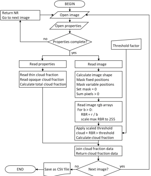
A flowchart of the specific Python tool proposed for analysing the TSI440 sky images in this
study and also used to develop the TSI_Analyser method has been exemplified in Figure 1.
Sky image integrity is a potential issue with pre-saved (i.e., historical) datasets, which on
some occasions, is expected to cause the photos to be malformed or even the acquired data to
be relatively incomplete[16] These corrupted files could also cause a given analysis tool to
cease its functions, generate inaccurate results and even ‘crash’ prior to the end of the final
execution, and provide to the user an erroneous dataset. To enable the Python tool to proceed
smoothly, an if-else conditional statement was developed, which was drawn from a common
feature for all coherent images. In the present research, the Python Imaging Library (PIL) was
file. If the common line was present, the Python tool proceeded as normal, else a ‘corrupted
file’ was recorded and analysis ceased for that file. and the next image file was read.
Once a sky image is shown to be non-corrupted, the image array is read using the NumPy
library via the OpenCV library’s imread command[25] and converted from the OpenCV’s
blue-green-red (BGR) to red-green-blue (RGB) to be used for further analysis. Reading each
image in OpenCV provides the required data of appropriate dimensions, including the 8-bit
colour channel array.[6,23,25] This step is of great importance as it can allow the data for each
image to be available as data arrays for current and also for further analysis. As the colour
channel array values are composed of 8-bit integer values, they are of the uint8 (8-bit
unsigned integer) data type in Python.[23,25] The OpenCV library then truncates uint8 values
outside of the possible colour intensities of 0 to 255 digital numbers.
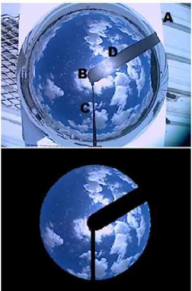
In designing the TSI_Analyser tool, a set of masks were applied to eliminate the non-sky
portions of the image, specifically, the background, camera housing, camera-arm and
sun-shield (see Figure 2 top image). The background, camera position and camera-arm were all in
fixed positions, hence a constant mask was made to mask these based on the dimensions of
the image and the objects’ position.[4] The background, which includes some of the horizon
due to the obstructions, was masked outside of a circle, as determined by an observationally
pre-determined constant radius, used as a proportion of the image height, from the image
centre, calculated using geometric functions from the NumPy library.[25,26] The camera
housing and camera-arm were masked using the circle and line functions of the OpenCV
library to provide the resultant image for further processing (Figure 2, bottom image). The
It should be noted that the sun-shield position is largely dependent on the solar azimuth, since
the reflective dome with the black band to obscure the sun rotates during the day to obscure
the solar disc.[5] This solar azimuth angle is therefore recorded in the properties text file when
using the TSI440 apparatus. The azimuth angle is also retrieved using the getline function of
the linecache library and is made into a line-based adaptive mask, where the position is
converted using trigonometric functions of the math library. This aims to convert the azimuth
angle to their unit circle equivalents and mask it as a line with a width of 60 pixels[4] (see
Figure 2, bottom image).
In atmospheric imaging devices such as the other forms of sky-imagers or smartphone-based
surveys, a properties text file may not be available, nor is the solar azimuth. However, the
date and the time that the picture was taken should be accessible either as part of the
filename, in the image properties or in an associated database. All of these properties can be
accessed using Python scripts and processes like the ones described for this research
methodology paper. The date and time of a sky-image and its geographical position can be
used to calculate the azimuth[4] by a relevant adapting code such as the one developed by
Michalsky[27] in the FORTRAN programming environment, which can be easily adapted to
Python.
In the Python TSI_Analyser tool, the red and blue colour channel arrays were selected for
further analysis and the masks were applied using the NumPy library. The sum of unmasked
pixels were determined. The potential ‘divide by zero error’ in the RBR ratio was avoided by
setting the RBR equal to 0 when the blue value was 0. In this method, the use of the
the array elements in all calculations.[21] The RBR pixel values were then scaled to increase
contrast to be within (0, 255).[6]
Considering the need to segregate the different cloud properties, a further adaptive mask was
designed to separate clear sky from the cloud components. The threshold was determined by
scaling a user-defined constant value with the maximum RBR value (RBRmax) calculated by
the tool for that particular image in the same manner that all the pixels were scaled, this is an
adaptation of the commonly used RBR transform. It is essential to statistically obtain the
user-defined constant value threshold by comparing a training data set with the TSI data[1],
particularly as the user-defined segmentation thresholds for the TSI440[22] may not be known.
This combination of fixed and adaptive thresholding was employed to take into consideration
the variations due to hardware, climate and the types of clouds.[2] The transformed data array
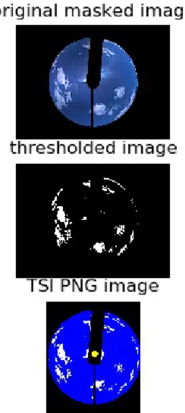
was then binarized.[6] The cloud fraction was determined for comparison with the previously
ground-truthed TSI readings by taking the cloud fraction differences.[22]
All data were integrated to the filename and saved as a row of a comma-separated value
(.csv) text files that can be accessed in any data analysis program, such as Microsoft Excel.
All sky-images in any directory with similarly defined filenames were searched for and
analysed in turn, then appended as a separate row in the .csv text file. Searching and
performing the same processes to multiple files in multiple directories for defined filenames
and types was performed using functions of the glob library. In the glob function, only those
image files at 5-minute intervals were taken by specifying that the final digit for the minutes
A practical measure of the efficiency of the Python tool was provided by the time taken to
execute the program, particularly the time of the components within it. To serve this purpose,
the timeit library provides a means to deduce how long each part of the Python tool takes to
execute, as with the entire program. Additionally, the time-efficiency of the Python tool was
tested since it was able to search through directories and perform the same processes to
multiple sky-images.
Results and Discussion: Application of TSI_Analyser
The optimum cloud/clear-sky adaptive threshold (T) to be used in this Python tool followed
the maximum RBR ratio (RBRmax) for an image, as follows:
T= 255k
RBRmax [4]
where k is between 0 – 1 and can be statistically determined for the specific case. In this
paper, a factor of k = 0.56 was used (Figure 3) based on a test on a training set of 2568
randomly selected images from different times of the day and different seasons, providing
suitable discrimination between clouds and the sky.
The segmentation of the images into cloud and sky was tested by comparing the resulting
percentage of cloud to the percentage of cloud obtained from the TSI440 software. The cloud
fractions from the TSI have been previously found to have an uncertainty of ±10% for a
minimum of 94% of the images.[28,29] The cloud percentages from a total of just over 42,000
images were compared to the cloud percentages from the TSI software and the median of the
difference was 0.74% with an interquartile range of -3.0% to 2.0%. The comparison showed
of the cases provided a difference that was within 5% of the TSI values. There was a strong
correlation of 0.93 between the original and calculated data. The cases with the bigger
differences are generally due to images with high level cloud, mist and dust. Just less than
2000 images were flagged as being corrupted, but these did not cause the program to cease
functionality.
The total time taken to execute the entire Python-based tool on a single sky-image averaged
to about 0.06 seconds on both computers used. However, testing increasingly larger datasets
in multiple directories showed that the total time taken was dependent on the number of files
analysed with a linear progressive function. The program was set to only analyse the data at
5-minute intervals from 5 am to 7 pm local time for the full 12-month dataset, calling on a
total of 42,084 sky-images; a task that was performed in just over 40 minutes.
Potential Limitations and Conclusion
Despite the efficacy of the proposed approach in terms of its major contribution to
atmospheric image analysis, speed and accuracy, there remain some limitations in terms of
running the TSI_Analyser, particularly when adapting the program to analyse the sky images
from other devices. Future users of this Python tool should ensure that a careful consideration
be given when developing parameters for the adaptive masks used in the approach. In any
iteration of the tool, the time taken in the program execution will depend on the processing
speed and available memory on the computer that the analysis is being performed.
In any sky image dataset, the presence of corrupt images is unfortunate, but these are likely to
occur on an ad-hoc basis. In this research paper, we were able to account for and correct two
image had failed to completely form. There may be other types of image corruptions that may
not be able to be anticipated in this methodology, and therefore, this opens a new window of
opportunity for further developing of the proposed TSI_Analyser Python tool.
In order to generate new knowledge on atmospheric dynamics, atmospheric scientists will
likely wish to review and utilise useful information from significant repositories of stored sky
images, just as we have done so for our 12-month sample dataset. These repositories often
have thousands of images and their associated files, which is far too much for them to be
analysed individually ‘by hand’. Therefore, a fast, efficient approach able to perform the
analysis has been developed and described, providing a useful contribution to future data
acquisition and analysis methodologies, particularly in the area of image analysis. The
present study shows that the proposed Python tool remained stable when searching through
the directories and analysing each sky image, gathering data about the segmentation
properties of the whole sky and clouds, taking just 0.06 seconds to complete each image – a
rate that remains consistent regardless of the number of images analysed. This resulted in
over 42,000 images being processed in 40 minutes. The proposed method described can be
adapted for other channel combinations[17] and to the other types of sky images and for other
properties, such as chromatic properties.
Acknowledgements: The authors thank Dr Ravinesh Deo for the productive discussions on
References
[1] Ghonima, M.S.; Urquhart, B.; Chow, C.W.; Shields, J.E.; Cazorla, A.; Kleissl, J. A method for cloud detection and opacity classification based on ground based sky imagery.
Atmos. Meas. Tech.2012, 5, 2881-2892.
[2] Li, Q.; Lu, W.; Yang, J. A hybrid thresholding algorithm for cloud detection on ground-based color images. J. Atmos. Ocean. Tech.2011, 28, 1286-1296.
[3] Heinle, A.; Macke, A.; Srivastav, A. Automatic cloud classification of whole sky imagers. Atmos. Meas. Tech.2010, 33, 557-567.
[4] Long, C.N.; Sabburg, J.; Calbó, J.; Pagés, D. Retrieving cloud characteristics from ground-based daytime color all-sky images. J. Atmos. Ocean. Tech.2006, 23(5), 633-652. [5] Parisi, A.V.; Sabburg, J.; Kimlin, M.G. Scattered and Filtered Solar UV Measurements;
Kluwer Academic Publishers: Dordrecht, 2004.
[6] Richardson Jr, W.; Krishnaswami, H.; Vega, R.; Cervantes, M. A low cost, edge computing, all-sky imager for cloud tracking and intra-hour irradiance forecasting.
Sustainability, 2017, 9, 482, doi:10.3390/su9040482.
[7] Chauvin, R.; Nou, J.; Thil, S.; Traoré, A.; Grieu, S. Cloud detection methodology based on a sky-imaging system, Energy Procedia, 2015, 69, 1970-1980.
[8] Spyranitos-Xioufis, E.; Mountzidou, A.; Papadopoulos, S.; Vrochidis, S.; Kompatsiaris, Y.; Georgoulias, A.R.; Alexandri, G.; Kartidis, K. Towards Improved Air Quality Monitoring using Publicly Available Sky Images. In Multimedia Tools and Applications for Environmental and Biodiversity Informatics,; Joly, A., Vrochidis, S., Karatzas, K., Karpinnen, A., Bonnet, P., Eds., Springer: Cham, 2018.
[9] Yang, J.; Min, Q.; Lu, W.; Ma, Y.; Yao, W.; Lu, T. An RGB channel operation for removal of the difference of atmospheric scattering and its application on total sky cloud detection. Atmos. Meas. Tech.2017, 10(3), 1191-1201.
[10] Yang, J.; Min, Q.; Lu, W.; Yao, W.; Ma, Y. An automated cloud detection method based on the green channel of total-sky visible images. Atmos. Meas. Tech.2015, 8(11), 4671-4679.
[11] Parisi, A.V.; Sabburg, J.; Turner, J.; Dunn, P.K. Cloud observations for the statistical evaluation of the UV index at Toowoomba, Australia. Int. J. Biomet. 2008, 52, 159-166. [12] Calbó, J.; González, J.A. Empirical studies of cloud effects on UV radiation: A
review. Reviews of Geophys.2005, 43(2). RG2002, doi: 10.1029/2004RG000155.
[13] Pfister, G.; McKenzie, R.L.; Liley, J.B.; Thomas, A.; Forgan, B.W.; Long, C.N. Cloud coverage based on all-sky imaging and its impact on surface solar irradiance. J. Appl. Meteorol.2003, 42, 1421-1434.
[14] McGonigle, A.J.S.; Wilkes, T.C.; Pering, T.D.; Willmott, J.R.; Cook, J.M.; Mims III, F.M.; Parisi, A.V. Smartphone spectrometers. Sensors, 2018, 18(1), 223, doi:10.3390/s18010223.
[15] Parisi, A.V.; Downs, N.J.; Igoe, D.P.; Turner, J. Characterisation of cloud cover with a smartphone camera. Inst. Sci. Tech.2015, 44(1), 23-34.
[16] Sabburg, J.; Wong, J. Evaluation of a ground-based camera system for use in surface irradiance measurement. J. Atmos. Ocean. Tech.1999, 16, 752-759.
[18] Dev, S.; Savoy, F.M.; Lee, Y.H.; Winkler, S. Rough-set-based color channel selection. IEEE Geosci. Rem. Sens. Lett. 2017, 14(1), 52-56.
[19] Shields, J.E.; Karr, M.E.; Johnson, R.W.; Burden, A.R. Day/night whole sky imagers for 24-h cloud and sky assessment: History and overview. Appl. Optics, 2013, 52(8), 1605-1616.
[20] Pawar, P.; Cortés, C.; Murray, C.; Kleissl, J. Detecting clear sky images. Sol. Energy,
2019, 183, 50-56.
[21] Jayadevan, V.T.; Rodriguez, J.J.; Cronin, A.D. A new contrast-enhancing feature for Cloud detection in ground-based sky images. J. Atmos. Ocean. Tech. 2015, 32, 209-219. [22] Slater, D.W.; Long, C.N.; Tooman, T.P. Total Sky Imager/Whole Sky Imager Cloud
Fraction Comparison. In 11th ARM Science Team Meeting Proceedings, Atlanta, Georgia, March 19-23, 2011.
[23] Oliphant, T.E. Python for scientific computing. Comp. Sci. Eng.2007, 9(3), 10-20. [24] Deo, R.C.; Downs, N.; Parisi, A.V.; Adamowski, J.; Quilty, J. Very short-term
reactive forecasting of the solar ultraviolet index using an extreme learning machine integrated with the solar zenith angle. Env. Res.2017, 155, 141-166.
[25] Van der Walt, S.; Schrönberger, J.L.; Nunez-Iglesias, J.; Boulogne, F.; Warner, J.D.; Yager, N.; Gouillart, E.; Yu, T. scikit-image: Image processing in Python. PeerJ, 2014, 2, e453. doi.org/10.7717/peerj.453.
[26] Van der Walt, S.; Colbert, C.; Varoquaux, G. The NumPy array: a structure for efficient numerical computation. Comp. Sci. Eng.2011, 13(2), 22-30.
[27] Michalsky, J.J. The astronomical almanac’s algorithm for approximate solar position (1950-2050). Sol. Energy, 1988, 40, 227-235.
[28] Long, C.N.; Slater, D.W.; Tooman, T. 2001. Total sky imager model 880 status and testing results. Report DOE/SC-ARM/TR-006. https://arm.gov/publications/tech_reports/ arm-tr-006.pdf (accessed March, 2019).
[29] Sabburg, J.; Long, C.N. Improved sky imaging for studies of enhanced UV irradiance.