A composite model and convex set coding technique for time-varying images

A COMPOSITE MODEL AND CONVEX SET CODING TECIINIQUE

FOR TIivlE-VARYING IMAGES

by

Peter Santago, II

Center for Communications and Signal Processing Department of Electrical Computer Engineering

North Carolina State University

May 1986

SANTAGO II, PETER. A Composite Model and Convex Set Coding Set Coding Technique for Time-Varying Images. (Under the direction of Sarah A. Raj ala.)

A coding technique is developed which uses convex sets to define image characteristics. The method of alternating projections onto convex sets is then employed to reconstruct images which exhibit the desired characteristics. A model for time-varying image difference pictures is also derived together with its rate dis-tortion function and this model isused for testing the coder.

Synthetic images generated from the model are presented. These images are shown to be in good agreement with actual images both visually and statistically. The rate distortion function indicates that most of the information of the difference picture is contained in the values of the moving pixels and not in their locations.

TABLE OF CONTENTS

1 MOTIVATION .

·1.1 Introduction .

1.2 Compression problem .

1.3 Modeling .

1.4 Proposed solution .

1.5 Outline of chapters .

2 BACKGROUND .

2.1 Introduction .

2.2 Coding .

2.2.1 Transform coding .

2.2.1.1 Introduction .

2.2.1.2 Selecting the basis vectors ..

2.2.1.3 Block transform coding .

2.2.1.4 Hybrid Coding .

2.2.1.5 Coefficient selection and quantization ..

2.2.2 Pixel domain coders .

2.2.2.1 Introduction .

2.2.2.2 Predictive coders .

2.2.2.3 Quantization .

2.2.2.4 Binary images .

2.2.3 Mixed domain coders .

2.2.4 Other coding techniques .

2.2.5 Comparison and pertinence to this research ..

2.3 Modeling .

2.4 Summary .

3 WAGE MODELING .

3.1 Introduction .

3.2 Actual sequences .

3.2.1 Noise estimation .

3.2.2 Motion Estimation .

3.3 Stationary Gauss-Markov .

3.3.1 Introduction .

3.3.2 Motion percentage .

3.3.3 Composite Model .

3.3.4 Clustering effect of the mask 51

3.3.4.1 Discussion 51

3.3.4.2 Clustering results of mask generation 54

3.3.5 Motion region statistics

00...

70 3.3.5.1 Using a Gauss-Markov image model... 72 3.3.5.2 Gauss-Markov model with motion parameters 72

3.3.5.3 Motion vector approximation 76

3.3.6 Synthetic image generation 77

3.4 Conclusions 77

4 RATE DISTORTION CALCULATIONS 79

4.1 Introduction 79

4.2 Rate distortion function for the mask 80

4.2.1 Probabilityof a mask error

0...

81

4.2.2 Mapping a mask error to image distortion 90

4.3 Rate distortion function for the moving region 92

4.4 Total rate distortion function 94

4.5 Conclusion 97

5 MIXED CODER 98

5.1 Introduction 98

5.2 Convex sets 98

5.2.1 Introduction 98

5.2.2 Projection 101

5.2.3 Method of Alternating Projections ..

00

00...

103 5.2.4 Projected Image Quality... 105

5.3 Convex set coders 106

5.4 Mixed Coder 111

5.4.1 Description of the implemented coder 111

5.4.2 Extended mixed coder 116

5.4.3 Frequency coefficient quantization and selection 118

5.4.4 Mask coding 119

5.4.5 Optimal solution 120

5.4.5.1 Discussion 120

5.4.5.2 Projection onto non-intersecting convex sets 122

5.5 Conclusions 125

6 CODING RESULTS 126

6.1 Introduction 126

6.2 Actual image single frame coding 127

vi

6.4 Actual sequence coding results 145

6.5 Discussion and conclusions 152

7 CONCLUSIONS AND FURTHER RESEARCH 155

7.1 Summary of research 155

7.2 Conclusions 156

7.3 Further research 157

8 REFERENCES.... 159

9 .APPENDIX 169

9.1 Appendix A: Optimal centers for translated energy sets 169 9.2 Appendix B: Convergence and minimization properties for

non-intersecting convex sets ...~~... 172

LIST OF FIGURES

Frame 0of BOBSJOB 27

Frame 30 of BOBS JOB 27

Frame 0 of MAP 28

Frame 30 of MAP 28

Noise statistics for BOBSJOB 29

Noise statistics for BOBS JOB 29

Full frame motion percentages for BOBSJOB 33

Full frame motion percentages for MAP 33

Windowed BOBSJOB frame 35

Windowed MAP frame 35

Windowed motion percentages for BOBSJOB 36

Windowed motion percentages for MAP 36

Actual mask for BOBSJOB 37

Actual mask for MAP 37

Gaussian tail cutoffs for 18.1% motion. 47

Synthetic difference picture mask 49

Synthetic difference picture mask 49

Synthetic difference picture mask 50

Synthetic difference picture mask 50

Actual image clustering 56

Actual image clustering 56

Actual image clustering 57

G1 clustering 58

G2 clustering 58

G3 clustering .. 59

G4 clustering .. 59

G1 clustering 62

G4 clustering 62

Actual image clustering 65

Actual image clustering 65

Actual image clustering 66

G1 clustering 67

G4 clustering 67

viii

Error regions for mask error 83

Graphic representation of Lagrangian 88

Mask rate distortion function 92

Moving region rate distortion function 94

Total rate distortion function 97

Convexity in two-space 100

Method of successive projections 104

Convex coder 107

Minkowski functional p,,(x)for convex set K 108

Simple mixed coder using POCS 113

Implemented mixed coder using

poes

115

Implemented mixed coder using NPOCS 118

Method of successive projections for non-intersecting convex sets 124

Coder comparisons for BOBSJOB 132

Actual BOBSJOB difference frame 133

Transform coded difference frame 133

NPOCS coded BOBS JOB difference frame 134

NPOCS coded BOBSJOB difference frame 134

NPOCS coded BOBSJOB difference frame 135

Improvement for NPOCS over transform for BOBSJOB 136 Improvement for NPOCS over transform for BOBSJOB 136

Coding comparison with actual rdf 141

Coding comparison with actual rdf 141

Improvement of NPOCS over transform 142

Improvement of NPOCS over transform 142

Original synthetic image 143

Transform coded image 143

NPOCS coded image 144

BOBSJOB sequence coding error 146

BOBSJOB sequence frame 20 original... 147

BOBSJOB sequence frame 20 transform coded 147

BOBSJOB sequence frame 20 NPOCS coded 148

M.AP

sequence coding error 149

M.AP

sequence frame 17 original 150

M.AP

sequence frame 17 transform coded . 150

LIST OF TABLES

BOBSJOB difference sequence noise covariances 31

MAP difference sequence noise covariances 31

BOBS JOB sequence covariances 43

MAP sequence covariances 43

BOBSJOB difference sequence covariances 43

MAP difference sequence covariances 43

Synthetic image covariances 55

Zero threshold mask correlations with 18.1

%

motion 61 Zero threshold mask correlations with motion correction 63 Non-zero threshold mask correlationswith 18.1

%

motion 64 BOBS JOB coding results with low change block problem .. 128 BOBSJOB coding results without low-change block problem 131 Synthetic coding results with low change block problem 139 Synthetic coding results without low change block problem 140

Coefficient statistics for 8xI6 pixel blocks 179

Bit assignment at 0.125 bits per pixel... 181 Bit assignment at0.25 bits per pixel... 181 Bit assignment at 0.375 bits per pixel... 181

Bit assignment at 0.5 bits per pixel 182

Bit assignment at 0.75 bits per pixel... 182

Bit assignment at I bits per pixel . 182

Bit assignment at 1.5 bits per pixel... 183

Bit assignment at 2 bits per pixel 183

Bit assignment at 2.5 bits per pixel... 183

Bit assignment at 3 bits per pixel... 184

Bit assignment at 3.5 bits per pixel... 184

CHAPTER 1

MOTIVATION

1.1. Introduction

This dissertation addresses two basic problems. The first involves the compression and transmission of time-varying images; in particular the compres-sion and transmiscompres-sion of digitized time sequences of monochrome images. The second problem isto determine an appropriate model which can be used to analyze and test the proposed coding algorithm.

The proposed solution for the compression problem is to utilize the method of projection onto convex sets(POeS) and an extension of this method to incorporate both frequency and pixel domain information. The modeling problem involves segmenting an image into changed and unchanged regions thereby forcing some nonstationarity in the scene.

solution for each problem is presented.

1.2. Compression problem

At this point it might be stated that the increased use of optical fibers elim-inates bandwidth as a major concern. This viewpoint ignores the fact that there is a large existing investment in older transmission media which can be used more effectively if the bandwidth is exploited more efficiently. Moreover, as with most new technologies, the bandwidth provided by optical fibers will no doubt soon be in much demand. In addition to this, satellite communication systems do not enjoy the luxury of connections to earth stations via hard links. It may be the case, however, that in short haul or local communication systems fibers may pre-clude the use of exotic compression algorithms.

Many factors indicate that as more bandwidth is provided, either by new technologies or by better compression methods, applications will be found to utilize this capability. Some of these uses include video teleconferencing, an increased number of television channels, and remotely piloted vehicles. It is also of little doubt that many other applications for time-varying image transmission will be discovered, both military and commercial [55].

3

The rate distortion function defines the minimum rate, typically in bits/time,

at which a certain type of signal needs to be transmitted in order to achieve a

given fidelity criteria [8]. This function is based on the probability distribution of

the various images which are to be transmitted and a measure of the quality of the

received images. Using rate distortion theory, the theoretical limit for transmission

can be determined for a given stochastic process which generates images or for an

image model. The rate distortion function can be found for various image models

and can then be compared with the distortion produced by the algorithms in

ques-tion. Rate distortion functions have been found for some systems, for example see

[61],

and are used in this dissertation for comparison and to analyze results.

If certain levels of distortion are allowed, as assumed above, then it is easily seen that this is one way of achieving bandwidth reduction. Compression can also be achieved by exploiting the redundancy in an image sequence, both within a

frame as well as between frames. IT one simply examines an image sequence

visu-ally or actuvisu-ally calculates the correlation, it is obvious that there is much

inter-frame and intrainter-frame redundancy. This redundancy property has been used by

many coders to reduce bit rates [65], and it is also utilized by the coder proposed in

this dissertation. Another important compression method is to predict motion

from frame to frame, and this technique may be used in conjunction with many of

the other coders including the one proposed here.

The reasonableness and realizability of the primary problem, compression, is

justification can be obtained by reading the background material in Chapter 2. In addition, compression has been achieved using both mathematical and subjective distortion measures.

1.3. Modeling

New coding techniques should offer advantages over existing methods. These advantages may provide a better rate distortion function for a given sequence type, may be more easily implemented, or may perform faster. In any event, the user must somehow be convinced of these properties. This maybe accomplished empir-ically by coding various sample sequences and comparing results. Indeed, this pro-vides a useful and necessary test for any new system. However, in conjunction with this should be some form of algorithm analysis which is born out by these experiments

In order to perform the analysis, general statements about the class of images that are to be coded need to be made. These general statements describe the image model and are usually in the form of image statistics. These models are nor-malty agreed upon by visual comparison with expected actual images, by checking the statistics of the model with those of actual images, or by showing that the model is mathematically tractable and seems to provide reasonable coding agree-ment when compared to coding actual image sequences. More likely a combination of reasons is used to arrive at a model. Regardless of how one decides, a model is

•

5

Given the need for a model, is it reasonable to assume that appropriate

models can be found? The following discussion shows that it is. By examining

Jain's review

[3.8],

it is obvious that many mathematical models are available. Further, many of these have been used successfully to produce and test

compres-sion algorithms. Another useful model can be derived by describing a time-varying

image sequence using translational motion as the basis. This representation has

been utilized to produce many motion compensation compression algorithms

[51].

The secondary problem addressed by this dissertation is to derive a model which

faithfully depicts the type of image sequences being coded, those containing

inter-frame difference pictures. Next a proposed solution to the compression and

model-ing problems is outlined in general terms.

1.4. Proposed solution

The solution proposed for the compression problem is initially derived by

visually examining interframe difference pictures, recognizing some significant

pro-perties, and utilizing the method of projection onto convex sets (POeS) to force the transmitted images to display these properties. In particular, interframe

difference pictures have large zero intensity regions and impulse-like nonzero

regions. By using interframe transform coding in conjunction with transmitting

the locations of the zero intensity regions, transmissions have been obtained with

significantly lower distortions than with interframe transform coding alone. In

short, the new system is an interframe hybrid transform coder which incorporates

both the square error and simple subjective viewing quality. The initial image sequence used was the head scene of a newscaster speaking and moving his head .

As stated, experimental results are promising and a full analysis of the method is presented in this dissertation. Also, work done by Roese and Pratt [67] shows that interframe hybrid coding can produce better results than three dimen-sional transform coding. This provides further justification for improving this cod-ing technique. In addition, transmitting the pixel domain information for the new coder seems adaptable to the use of run length coding. This is covered more throughly in Chapter 2.

In this dissertation, the use of

poes

has also been extended to nonintersect-ing convex sets to produce an optimal least squares solution. This optimal pro-cedure also presents less of a computational burden by requiring iteration only at the transmitter.

7

be thought of as the moving and nonmoving areas of the scene. Mathematical measures are defined which can be used to test the appropriateness of the model.

Synthetic images were generated and coded using the new method. The results of coding these synthetic are close to the results produced by coding actual image sequences. A complete analysis is given in Chapter 6.

1.5. Outline of ehapbera

CHAPTER 2

BACKGROUND

2.1. Introduetion

Image sequence compression research has produced a tremendous amount of literature over the past ten to fifteen years, and any detailed review of all of this work is beyond the scope of this dissertation. There are many good reviews on the topic including Jain [38], Habibi [28], Netravali [55], and Pratt [65]. The paper by Hsing and Tzou [34] is particularly concise and provides an excellent quick over-view of the topic. The background report given here reover-views the basic concepts of various types of compression techniques which are most pertinent to this disserta-tion and references some of the basic research on these topics. In particular the system presented here utilizes a mixed coder which combines interframe hybrid transform and pixel domain coding techniques for time-varying image sequences.

2.2. Coding

3.2.1. Transform coding

9

2.2.1.1. Introduetion

A digitized NxN image can be viewed as a vector in RNl. In the pixel domain each pixel intensity value is a component of the vector or can be considered as the coefficient for a standard basis vector representation of the image. A discussion of vector space formulation for images can be found in Pratt's paper [63]. A transform coder effectively performs a change of base on the image vector. That is, the N2 transform components are coefficients for a new set of basis vectors or basis images. A transformation is done in order to gain some coding advantage by com-pacting energy or information into fewer components or by making the coded image less susceptible to errors. Typically the transforms used are unitary for the basis orthogonality, the ease of calculating the coefficients, and for having an easily defined inverse. Also, such a transform is energy and information preserving [6].

2.2.1.2. Seleeting the basis veetora

derivation of this transform can be found in [18]. The difficulty with this transform is that it is computationally burdensome and requires statistics of the sequence. To see this, one only needs to recognize that the covariance is N2xN2.

Another transform which is optimal in the least squares sense is given by singular value decomposition. In this method, an NxN image is represented by the weighted sum of N rank one matrices (images). If L

<

N of these images are transmitted, the sum of these L images minimizes the error between the actual image and the sum of any other L rank one images. These basis matrices must be transmitted for each frame since they are not a function of the sequence statistics. Being rank one, however, each basis image can be written as the outer product of two length N vectors. The performance of this coding method generally is not as good as for transform coding [64].

Two dimensional transform coding was first introduced by Andrews and Pratt [5]. In this work a Fourier transform is performed on an entire image for coding. It was shown that errors (channel or quantization) in the coefficients were less noticeable since they tended to be distributed over the entire image. It was also noted that more energy in the image was compacted into fewer coefficients than in the pixel domain representation. This observation addresses the exact problem posed by the Karhunen-Loeve formulation. Further, the Fourier transform has a fast implementation.

11

advantages. For example, the cosine transform eliminated the blocking problem by forcing symmetry in the image to be transformed [65]. Examples of more efficient transforms are the slant, Haar, and the Hadamard and a review of these can be found in

[64).

More information on general orthogonal transforms and gen-eral fast transforms are in [19], [21], and [20].

Since transforms which were computationally feasible were shown also to be useful, it remained to be shown how good they were. In particular, how did these fast transforms compare to the Karhunen-Loeve transform? One basic drawback of transform coding is the blocking effect caused by Gibb's phenomenon at the image edges as stated above. Forcing symmetry by unfolding the image produces significant improvement. This was shown by using the cosine transform on the symmetric version [2). Perhaps more importantly, however, is that the cosine transform was shown to approach the Karhunen-Loeve under certain practical assumptions [65]. In light of this result, it does not seem advantageous to continue the search for further transform types [65]. The next question which was asked is what is the effect of transforming blocks of the image instead of one entire NxN frame is discussed?

2.2.1.1. Bloek transform eoding

spatial correlation distance in the image. However, as Pratt [65] points out, this is not valid since it ignores the correlation between adjacent blocks at common edges. The problem, then, is to define a valid tradeoff between computation and compres-sion. Tables comparing the effects of various block sizes can be found in [64]. In fact, the cosine and the Karhunen-Loeve transforms give practically identical errors for a Markov image model and very small block sizes, say 8x8 pixels. As the block size increases slightly, as low as 16x16, the Fourier, slant, Haar, and Hadamard are shown to be within

1%

of the Karhunen-Loeve mean square error. As stated earlier, the pertinence of these facts to this dissertation is that the type of transform and the block size are not the most important factors for the algo-rithm being analyzed.

13 2.2.1.4. Hybrid Coding

Hybrid coding, also referred to as hybrid transform/predictive or hybrid transform/DPCM coding, is a combination of transform and predictive coding methods. The transform coefficients of a block are predicted using coefficients of nearby blocks in space or in time. Using spatially related blocks is known as intraframe hybrid coding and was introduced by Habibi

[27].

Using temporally adjacent blocks is called interframe or hybrid transform/DPCM and was first used by Roese

[67].

The method presented in this dissertation is a type of hybrid coder since it operates on the difference picture. The prediction is then the previous frame and so only the errors in the coefficients need to be transmitted which is identical to sending the coefficients of the difference picture as the transforms used are linear. Some general results concerning hybrid coders have been found and these are stated next.

Typically, intraframe hybrid coding does not provide performance which is as good as two-dimensional transform coding, but requires simpler hardware. In comparison, interframe hybrid coding improvement can perform better than two-dimensional transform as well as three-two-dimensional transform coding (apply the transform in the temporal as well as in the two spatial directions)

[67].

However, using a Gauss-Markov model, Pratt [64] indicates that three-dimensional transform coding should theoretically be better than hybrid interframe coding.

to these problems is much the same as for other coding methods. The main ques-tion to be answered for hybrid coders is that of determining the temporal and spa-tial correlation of various coefficients. Analysis and some results of this problem can be found in [67] and

[61].

Pearlman [61] states that there seems to be room for improvement at intermediate rates, and this is the region for which the coder described in this dissertation shows a gain.

2.2.1.5. Coeflieient seleetion and quantisation

The final issues in the design of a transform coder are those of selecting and quantizing the L out of N2 coefficients to be transmitted. The selection should be of those coefficients which will produce the minimum mean square error, the L largest. The method which uses this approach is called threshold sampling. The drawback is that an address indicating which coefficients are being transmitted must also be sent, thereby reducing the number of bits available at a fixed transmission rate for the coefficients themselves.

16

Quantization of the coefficients addresses the problem of how many bits should be assigned to each coefficient, given a fixed number of bits for transmitting each frame or image, in order to minimize the error at the receiver. This problem was solved by Max [48] for average error over all of the components of a vector and for each component by Huang [35]. These problems were expanded upon by Segall [75]. For un correlated coefficients, the number of bits assigned to each coefficient

is a function of the log of the variance of that coefficient [64] and

[75].

Many transform coders use an a priori bit assignment related to the zig zag selection pat-tern mentioned earlier which is easy

t?

implements and performs well

[64].

In gen-eral, a fixed level quantizer performs well when compared with the optimum mean square error quantizer [80]. This research employs a uniform quantizer with bit assignment for various transmission rates which is a function of the variance of the coefficient. This assignment, then, also performs coefficient selection.

2.2.2. Pixel domain eodees

2.2.2.1. Introduetion

2.2.2.2. Predictive coders

Better pixel domain coders than the one just mentioned attempt to predict pixels values from spatially and/or temporally adjacent pixels. In this way the coders need only transmit the error sequence which generally requires fewer bits than the full intensity sequence. For examples see [57] and [9].

One issue concerning this coding technique is to decide, for each pixel, which of its neighbors to use as predictors. That is, should spatially or temporally related pixels or both be used? Further, one could ask which pixels in each one of these dimensions should be used, although the nearest pixels to the one being predicted are the most reasonable. O'Neal [57], using DPCM techniques, shows little gain by using spatially related pixels more than

1

pixel away. Alexander

[4]

uses linear predictive coding (LPC) and three neighborhood pixels to predict and shows simi-lar results for a two pixel neighborhood. If a first order Markov process is used to model the image, then it is obvious that only one pixel in each dimension is needed. Maragos [46] also produces good reduction using two-dimensional LPC and an adaptive quantizer. He shows than three coefficients are sufficient to achieve good rate distortion characteristics applied over blocks of 16x16 pixels. The paper also gives a good overall analysis of two dimensional linear prediction.

2.2.2.1. Quanti.ation

17

allocation seems to be a good choice for comparing coding algorithms objectively. A uniform quantizer is more easily implemented and can be made non-uniform with a compander design. Quantizing with respect to visual error criteria has also been done by Scoville

[74]

and Netravali [52]. This method seems reasonable for implementing a real system if the criteria are not too complex. It can, however, be more difficult to analyze or to compute a rate distortion function for these methods. There are certain cases of visual fidelity criteria which do not present undo analysis problems such as weighted frequency measures. When this type of error criterion is used for an image model, such as the Gauss-Markov, the rate dis-tortion function can still be determined in a straightforward manner

[16].

As in transform coding, equilevel quantizing performs well [80].

Predictive or adaptive quantization takes advantage of the error sequence redundancy by adjusting the quantization levels dynamically. The choice of quantization strategy seems to be dictated by need as well as the allowed complex-ity of the system. This dissertation utilizes the more simple quantization schemes for the mathematical tractability as well as for comparison with other coding sys-tems. Also, as stated above, little is gained by employing exceedingly complex quantization schemes.

2.2.2.4. Binary images

zero and nonzero regions of the difference picture. This binary type of sequence is often well suited to run length coding. A chapter by Arps in [65] reviews tech-niques of errorless coding for images. The proposed coder makes use of existing methods for coding the zero regions of the difference picture rather than attempt-ing to define new techniques. Pratt

[64]

summarizes expected results of run coding under various conditions and states the possibility of a ten to one bit reduction for two dimensional run length coding on binary images.

2.2.3. Mixed domain coders

Coders which utilize both pixel and frequency domain information have received little study. This idea has gotten much attention in the field of image reconstruction [85]. One attempt at this type of coding was done by Yan and Sakrison [84] using a two component image model. A straight line fit was formed for sections of each scan line and transmitted. This fit was subtracted from the original line and the remainder was transform coded. The receiver then combined the two transmitted signals. Experimental results are given showing subjective improvement as well as mean square error and weighted mean square error reduc-tion. There is no rate distortion calculation or synthetic image coding.

19

difference pictures and this dissertation extends that work. The paper shows

significant improvement over interframe transform coding for some bit rates.

2.2.4. Other coding teehniques

There have been many coding techniques proposed and tested over the past

years for video sequences and the summaries listed in the reference section cover

the important ones. .Perhaps the most widely used and studied is motion

compen-sation coding. In short, pixel intensities are assigned by attempting to predict the motion in the image sequence. Moorhead

[51]

gives a good up-to-date background study of these algorithms. A nice feature of this method is that it can be incor-porated into other methods such as the one in this dissertation. The motion

pred-iction can improve the coder by giving a better initial estimate. Further, if back-ward motion compensation is used, this improvement can be achieved without

additional bandwidth requirements

[71].

Frame replenishment coding only transmits those pixels which have changed

significantly from one frame to the next. This means that the addresses of the

changed pixels must also be sent. Compression can achieved using this technique

down to one bit per pixel with excellent results except for periods of excessive motion

[64].

One problemwith this method is that the method normally requires a variable bit rate.

Human visual system

(HVS)

coders incorporate subjective quality measures

transmitted. By filtering according to HVS parameters before coding, the amount

of information to be transmitted can be reduced and conventional coding schemes be used after the filter. It seems probable that HVS coding will have to be utilized to achieve very low bit rate transmission. See [30] and [78] for discussions of this topic.

2.2.6. Comparison or eoding methods

Comparing the various coding systems is difficult to say the least. In order to get a common denominator, a distortion measure must be agreed upon so that rate distortion functions, discussed in Chapter 4, can be derived for each coding method. Also, an appropriate image model which is mathematically tractable and provides a faithful representation of image sequences must be found. Typically the square error criteria and a Gauss-Markov random field are used. The square error measure is also used in this dissertation, however, actual image results are given so that the subjective quality can be seen. The Gauss-Markov model is of question-able value to the new coding technique to be presented and is discussed more com-pletely in the next section and in Chapter 3.

21 The relative position of motion compensation coding is a little more difficult

to define. However many low bit rate coders have been implemented using this

procedure [34]. In this same reference, Hsing concludes that motion compensation techniques as well as hybrid transform/predictive coding are promising for further

compression. The proposed coder improves the hybrid method for certain rates.

More importantly, it seems to be very well suited to perform in conjunction with

motion compensation coders, since these types of coders produce a difference

pic-ture which should be even more amenable to coding by the new mixed coding

method.

2.3. Modeling

In his paper on mathematical image models, Jain [39] states that the type of model needed for compression studies is one which deals with distortion criteria

and images as information sources. In [70] the authors indicate that specifying a

distortion measure that is meaningful and tractable is a major difficulty. This may

also be stated for an image model as well. It must be a faithful representation of

the desired sequence type yet must also be analyzable. Further, the model should

allow for synthetic sequence generation so that actual coding results may be

obtained. In addition to Jain's review on models, Rosenfeld and Davis [68] also

cover the area.

For the purpose of this dissertation, the model should, as Jain states, regard

images as an information source. That is, the spatial and temporal relation among

purpose is the three dimensional homogeneous Gauss-Markov representation [39]. Pearlman [61] uses this model with a separable correlation to analyze interframe hybrid coding algorithms and to derive rate distortions functions for these. O'Neal [58] has an analysis for an isotropic correlation.

Although these models are useful for analyzing many compression schemes, they are not appropriate for the proposed coder. The problem is that the statistics are spread over the entire frame, and therefore the images do not contain the correct properties of difference pictures: large zero regions and impulse-like nonzero regions. For this reason, the new coder will not perform well on these models although good results are obtained for actual image sequences. A thorough investigation of this problem is given in Chapter 3.

Non-stationary models have been used in image segmentation research [68]. Rajala

[17]

segments an image for restoration purposes based on intensity slopes within regions of the image. The difficulty with these schemes for coding purposes is that they are not directed toward calculation of rate distortion functions or gen-erating synthetic images.

23

to analyze.

The approach taken here is to generate a binary mask based on the amount of motion in a scene indicating changed and unchanged areas. The statistics are dis-tinct between regions and the same within a region. This solution presents a tract-able compromise and is discussed fully in Chapter 3. Cafforio and Rocca [11] used this approach for segmenting an image into moving and nonmoving regions. They assumed each pixel was in one of these two states, moving or non-moving, and that the state of the next pixel was determined by a Markov process. That is, they assigned probabilities for moving from one state to the other or staying in the same state. Additional information on segmenting images using Markov models can be found in Hansen and Elliott's paper

[31].

2.4. Summary

quantization method, or the block size. This allows the research to concentrate on the proper trade-offs between domains.

For the pixel domain section of the coder, techniques should concentrate on those used for binary image transmission. The method chosen should be one that already has been developed; perhaps adapted to the statistics of the binary images expected. Again this allows the research effort to be on the new coding method.

25

CHAPTER 3 IMAGE MODELING

3.1. Introduetion

This chapter contains development and discussion of the image model which will be used later for analysis of the new coding algorithm. The purpose of this development is to derive an appropriate model which can be used to produce a meaningful analysis of the rate distortion limits of the mixed coder. Appropriate in this sense means both a mathematically tractable analysis tool and a faithful representation of the difference picture which contains large zero regions and clustered non-zero regions.

The first part of this chapter covers some preliminaries concerning the actual image sequences used for this research. Also discussed is how the percentage of motion is calculated and distributed within frames. Following this, the difference picture model is presented.

The appropriateness of the model is examined initially by showing how the probability of changed values can be matched to the motion percentage. The clus-tering effects of these changed pixels are then presented and compared with actual sequences using a probability and a correlation measure. A section is then included which used the Gauss-Markov model to generate statistics for the moving regions in a sequence. Finally, an explanation is given on how to use the composite model in order to produce synthetic images.

3.2. Aetual sequenees

1.2.1. Noise estimation

dis-Figure 3.1a: Frame 0 of BOBS JOB.

Figure 3.1b: Frame 30 of BOBSJOB.

Figure 3.1c: Frame 0 of MAP.

~ 0 Loft ""=0 .:-~ ca ~ ~

-

~

-

...

~ C) CD .JJ 0 C- O-~ 0 LD ~ 0 0 -~O

He.n :a 0.06

SiS"'. • 1.55

-l.~ -2.~ 0 2.~

Noise ini::eneity

10

29

Figure 3.2a: Noise statistics for BOBSJOB.

~

o~---.

He.n .. 0.01

S19111. • 2.03

o ~---....,.._'-:~---r----

...

-'--""----"""'---""-~==----'---~

-JoO -l.~ -2.~ a 2.~

Noieo i.ni::ene i ty

Figure 3.2b: Noise statistics for MAP .

tributed.

These statistics were generated by examining the difference pictures in regions where there was known to be no motion; thus all changes should be due only ~o

noise. This was done by taking the difference between adjacent frames for the specified region. Any nonzero values should be due to noise, so the sample mean value and variance were calculated using these difference values. The noise vari-ance for "the MAP sequence is somewhat higher than for BOBSJOB. The MAP sequence, however, has a textured background and therefore any camera jitter would contribute much more to increasing the variance in this sequence versus BOBS JOB. A simple block matching motion compensation scheme was employed in an attempt to correct any possible jitter problem. The correction scheme did not affect the statistics for either sequence.

In both sequences the noise appears to have a Gaussian shape, and when a true Gaussian with zero mean and the same variance is plotted with the sample noise graphs, there is no noticeable difference. The autocorrelation was also deter-mined and is given for various lags in table 3.1.. The autocorrelation is defined by the following:

uncorre-Table 3.1a. BOBSJOBdifference sequence noise covariances.

(k' ,I' ,t') (0,0,0) (0,1,0) (l,O,O) (I, 1,0) (0,0,1) (0,1,1) (1,0,1) (1,1,1) covariance 2.417 -.2422 -.0251 -.0380 -1.228 .1408 .0529 .0307 Inormalizedl 1 .1002 .0104 .0157 .5078 .0582 .0219 .0127

Table 3.1b. MAP difference sequence noise covariances.

[k',I',t') (0.0,0) (0,1,0) (1,0,0) (1,1,0) (0,0,1) (0,1,1) (1,0,1) (1,1,1) covariance 4.248 -.3153 -.0100 -.0193 -2.115 .2087 -.0103 .0019 bormalizedl 1 .0742 .0023 .0045 .4979 .0491 .0024 .0004

0;

lated and Gaussian.

3.2.2. Motion Estimation

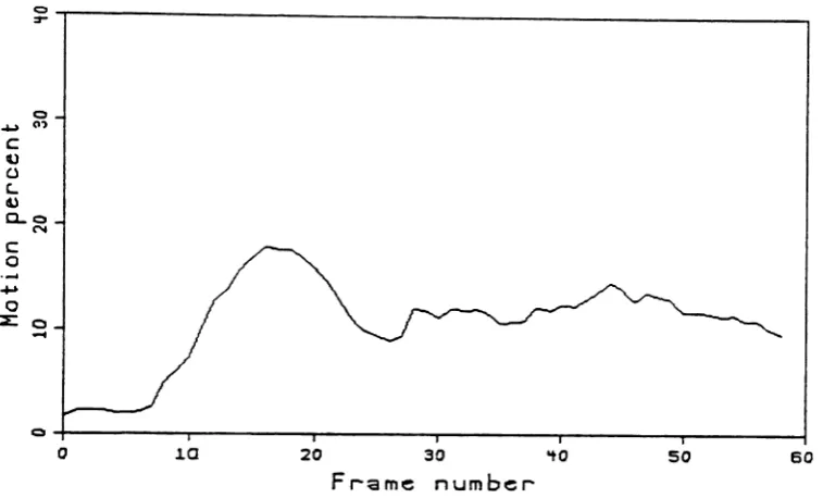
Motion is normally found by counting the number of changed pixels which are probably not changed due to noise. That is, a change in pixel intensity higher than say twice the noise standard deviation. The percentages, given in figure 3.3a,b, are based on a changed value of more than 3 in magnitude from frame-to-frame and a frame size of 282x484, and are due to [51]. For the case of the BOBSJOB sequence, this change of 3 amounts to about twice the standard deviation of the noise in the difference picture; for the MAP sequence it is somewhat less. Further there could also be changes due to motion with values

:::;131.

In fact, using this value has a much to do with representing perceivable changes, being consistent with other research, and to keep the coding algorithm simple as it does with being a true representation of motion. Possibly a better approach would be to first median filter the difference to eliminate isolated changes which are likely due to noise. In any event, these percentages give reasonable approximate values to use when gen-erating an image model and synthetic images.

~T---33

Q - r - - - - -...

----....,..---...,...---r---_---J

o .10 20 30 ~O

Fr-ame number

50 60

Figure 3.3a: Full frame motion percentages for BOBSJOB.

o~-_---_

~

Q-J-_ _

---.---,---r---...,...---r---t

o 10 20 30 ~o

Frame

number-so 60

BOBS JOB and the MAP sequence. Examples of the windows of this size are shown in figure 3.4 The 256x320 window allows for the motion to be fully contained and still have enough background to be in agreement with normal teleconferencing type sequences. The percent of motion found in the sequences for the windows is given in figure 3.5a,b and all further motion percentages will be given with an image size of 256x320. Also, when reference is made to BOBSJOB and MAP, this will now imply the sequence formed by the 256x320 window of the original sequence.

Perhaps smaller windows could be employed with even higher motion percen-tages for analysis and simulation and this would certainly reduce the computa-tional load. It was found, however, that the statistics generated for much smaller windows were not very robust for the necessary correlations. A smaller window also produces artificial clustering effects which are not found in the actual sequences used.

Figure 3.4a: Windowed BOBSJOB frame.

~~~_ _Figure 3.4b: Windowed MAP frame.

o _ - - - ,

~

C)-+---~----__._----_.,..----___r----~.__---~

o 10 20 30 ~O

Fr-ame

number-50 60

Figure 3.5a: Windowed motion percentages for BOBSJOB.

~

o % : 0

...

0 - _ _- - - . .

~

c:

o

C)-+---..---..---....,.---,---~---4

o 10 20 30 ~o

Frame

number-50 60

Figure 3.6a: Actual mask for BOBSJOB, threshold=3.

Figure 3.6b: Actual mask for ?vfAP,threshold=3.

3.3. Stationary Gauss-Markov

3.3.1. Introduction

The model to be analyzed in this section is well known and is given by a three dimensional, separable, homogeneous Gauss-Markov process [61]. An image sequence can be described by a random field, x , where the x(k,l,t) are random variables indicating the pixel intensities at location k,l,t, the two spatial and one temporal direction, respectively (k,I, and t are integers appropriate for the bounds of the image sequence). They are assumed to be identically distributed jointly nor-mal variates with the joint density function given by the following (the random field x of size N is indexed here by a single value).

-N

pz(x)

=

(21r)

2 ICI-1exp{-lh[x-fLz]TC-1[x-p.z]}

(3.2)

where superscript T indicates transpose, C is the covariance, ILz is the mean vec-tor,

kJl

is its determinant, and x=[X1X2 ... XN]t. Being jointly normal, the members of x are also marginally normal [59], i.e., x(k,l,t) E N( ....%,O'z). The autocorrela-tion of this process is given by:

Rz(k',l',t')

=

E{x(k,l,t)x(k+k' ,1+1' ,t+t')}

39

(

1

]3

1i' rr 1i

s,

=

21T

!'lr.L.L

max[0,lhlog2S(Wl,W2,W3)/O)dwldw2dw3

where

SO

is the spectral density of the random field x given by:

(3.4)

(3.5)

(3.6)

2 3 ( (l-ai

2

)

l

S(w1, W2 , w 3 ) = uz.n -1T~(J)i:51T • =1 (1 - 2a ._Icosw ._I

+

a_I

.2)

and 0<9 <ess sup S(Wl,W2,W3)' where ess sup is the essential supremum. The rate distortion function is covered completely in Chapter 4.

This model is also valuable since a synthetic image displaying these statistics can be generated using the following autoregressive process

[61].

x(k,l,t)

=

a1x (k - I ,1,t )+ a2x (k ,I - 1,t )+ a3x (k ,l ,t - l )

- ala2 x(k-I,l-l,t)-_{a l}aax(k-1,I,t-1)-a2aax(k,1-I,t-1)

+

al a2 aax(k-I,I-I,t -1)+bn(k,1

,t)

where n(k,l,

t)

is white Gaussian noise and b is chosen such that

(3.7)

(3.8) In order for the random field to have the proper variance. The question now becomes, can a good model be derived for the difference picture using the Gauss-Markov model as the starting point? The term "good" here is defined as providing the characteristics laid out in the introduction to this chapter.

To form an interframe difference picture sequence, a new random field, z, 1S

formed according to the following:

z(k,l,t) = x(k,l,t) - ax(k,l,t-l)

where a is a constant. If(1=1, then

(3.10) This produces a zero mean field as may be desired for the difference picture but leaves correlation in the temporal direction, i.e.,

Rz(k',I',t')

=

_{cr;[2Rz(k' ,I' ,t' )-R%(k' ,l'} .t' +l)-R%(k' ,I'

,t'

-1)]

=

CJ';a~A:'laJl'l (2aJ"l- aJt'+11_aJ"-11) (3.11)

where R; is the autocorrelation. It should also be noted that the random field z in this case is not Gauss-Markov

[42].

The temporal correlation can be removed if

Rz(k',I',t')

=

(1-a:)CJ';a~A:'latI8(t')

(3.12)

where 8() is the unit sample function. This form for z , however, does not have zero mean, i.e.,

z(

k ,I

,t)

EN((1-a3)f.Lz,0"%(1-

al

)~)

As will be seen, though, f.L_z is close to zero for useful values of a3.

(3.13)

41 3.3.2. Motion percentage

Once a model has been chosen, it is necessary to check whether or not the difference picture sequence produced by this method is useful for analyzing the proposed coder. In this section, the probability of nonzero pixel values is examined for the coder to see if it agrees with that produced by actual image sequences. Usually a zero is considered to be a pixel which has not undergone a significant change from one frame to the next. "Significant" is normally defined in terms of the noise in the sequence. If white Gaussian noise is present, say n EN(O,an), then a significant change may be a pixel which has changed in magnitude by more than 20'n' particularly if the pixel intensity changes due to motion are high relative to the noise. In the present case, noise is not considered and so a significant change may be thought of as a pixel intensity magnitude in the difference picture of one or more since all changes will be due to motion. It may seem that a change of any amount should be included, however, the pixel intensities are scanned as integer values. By adding noise, the results in the next paragraph are not significantly altered.

If there is 10% motion between two frames, then 90% of the pixels should be unchanged or 90% of the difference picture pixels should have the value of zero (in the open interval (-1,1)). Suppose an image sequence is generated using the Gauss-Markov model with al

=

a2= a3=O.9 and x(k,l,t) E N(128,SO) (these values

(actually the correlation coefficients) from actual sequences and difference picture sequences are given in table 3.2. If ex=1, from equation 3.9, then z(k,l,t) E N(O,22.36) and the probability of getting a value in the interval (-1,1) is only 0.036. This estimate is also somewhat generous in that it assumes truncation of intensity values rather that rounding which would give the interval for the probability to be only (-.5,.5).

The reason for this low probability is that the model tends to spread the correlation evenly over the entire image when in fact the difference picture is highly nonstationary. As it stands, this model is just not a very good one for gen-erating difference pictures. Even if the statistics are calculated for the difference pictures directly and the model used with these, the correlation is still too evenly distributed. Even with the drawbacks of this model, it is possible to correct the problem with the percent of motion. That is, the correct probability of an unchanged element can be forced by adjusting various parameters of the density or correlation functions of the pixel intensities.

Using the temporally decorrelating form for producing the difference picture,

a=aJ' then z is as in equation (3.12). Given a mean and variance for the actual image sequence, fixed IJ.% and (J'z»the only parameter which can be altered to affect

the probability of zero intensity pixels in the difference picture is a3. Letting M

represent the fractional amount of motion in the image, the value of a3 is adjusted

Table 3.2a. BOBSJOBsequence covariances.

(k',l',t') (0,0,0) (0,1,0) (1,0,0) (1,1,0) (0,0,1) (0,1,1) (1,0,1 ) (1,1,1)

covariance 2676 2645 2632 2611 2648 2623 2630 2612

lnormalizedJ 1 .9882 .9832 .9756 .9892 .9800 .9827 .9761

Table 3.2b. MAP sequence covariances.

(k',I',t') (0,0,0) (0,1,0) (1,0,0) (1,1,0) (0,0,1) (0,1,1) (1,0,1) (1,1,1)

covariance 1697 1677 1667 1653 1648 1653 1635 1637

~ormalizedl 1 .9882 .9822 .9740 .9711 .9742 .9635 .9646

Table 3.2c. BOBSJOB difference sequence covariances.

(k' ,l',t') (0,0,0) (0,1,0) (1,0,0) (1,1,0) (0,0,1) (0,1,1) (1,0,1) (1,1,1) covariance 55.32 49.13 36.43 34.87 19.60 22.1.) 31.07 30.73 lnormalizedJ 1 .8880 .6585 .6303 .3542 .4003 .5617 .5555

Table 3.2d. MAP difference sequence covariances.

[k ',I',t') (0,0,0) (0,1,0) (1,0,0) (1,1,0) (0,0,1) (0,1,1) (1,0,1) (1,1,1) covariance 91.95 79.26 57.98 53.50 15.63 25.24 21.86 24.78 Inormalizedl 1 .8619 .6306 .5818 .1700 .2744 .2377 .2695

Pr {

I

z

I;;:::

I}

=

M or Pr {z ;;:::I}

=

M

2

Let w be a random variable such that w E N(O,l). Then find a3such that

(3.14)

1-(l-a3)J.Lx M

Pr{w~ }

=

-(J%(1-a:)~ 2

This is found be solving

(3.15)

l-(l-a )110 M

1 - er] ( 3 r-z )

=

-(J%(l-aiYJ2

2 (3.16)

where

(3.17)

t2

2

dt

x

erf(x)

=

1

f

e

(21T)~ -00

This can be most easily solved using tables for the standard normal distribution, in

which case the solution for a3 becomes

(3.18) 1-(l-a3)J.Lz

=

R

(J%(l-ai)l4

where R is found in the tables working backwards from the given probability. That is, R is the value on the Gaussian tail which corresponding to having the proper motion percentage under the tail. Using the quadratic formula

J.Lz (J.L%-1)+~;(muz-1)2 - (R2(7:

+ ,...;)(

1-2J.Lz

+

I.L; -

R2(1

;YI2

R2cr_%2

+

11 ._,-z2

Some typical values of a3 are given below for 15% motion.

(3.19)

I.L%

=

128 J.Lz

=

128

Jel%=128

(J

z=20

{1z=40

(7%=60

a3=.999095

a3=.999730

a3=·999875

Note that moderate changes in {1% require very small changes in a3. Also, the

45

synthetic images and retain other necessary statistics. Further, it is nearly impos-sible to control the value of a3 to the four significant accuracy needed to produce

the proper values of cr:z: •

Although a3 can be found and the correct probability achieved, the (J"z

pro-duced is not typical for a motion sequence. In a 15% motion frame with the mean square change for pixel intensities equal to 225, crz would be 5.8. Using the model with al=a2=0.9, J.Lx=128, and (1%=40, then a , should have the value 0.93. If noise is present with a reasonable variance, say (J"n=1.5 as determined for one

actual sequence, this noise would completely dominate the motion changes. The value of az could be made more reasonable by altering cr:z:. This would, however, force the value of (J':z: not to be representative of actual image sequences. In

addi-tion, the correlation would not be correct since it would still be stationary over the entire image. The correct correlation for the difference picture should have one form for the changed region and uncorrelated for the zero or noise only area. As

stated before, the model is not very effective in its present form even if the image sequences were normalized to these lower values for z.

l.a.l. Composite Model

It is possible to use the previous model as the first stage of a more complex one, thereby retaining some of the analytic simplicity of the Gauss-Markov form.

changed. The mask can be produced by first generating a two-dimensional ran-dom field, z, using the autocorrelation as in equation (3.12) but without the time subscript since there is no temporal dependence. The values of a1and a2 are set as needed for the clustering effect for the moving regions.

Binary mask values are generated by assigning either a one or a zero to each pixel in the field z indicating its presence or absence in the changed region. This can be done by determining a negative and positive cutoff point on the normal curve so that the area under the remaining tails is equal to the motion percent (see figure 3.7). These cutoffs are assumed to be equal in magnitude. The generated mask, m, is given be the following:

{

I , Iz(k,I)I>cutoff

m_{( , ) -}k I - _{0, IZ(k,I)1}

<cutoff (3.20)

For example, if the random field contains variates in N(O,l) and 15% motion is desired, then, using tables for the normal distribution, all values outside the interval [- .19,.19] would be assumed changed and all others unchanged. Masks using this approach are shown in figures 3.8. These masks assume 18.1% motion. The values of al and a2 are equal in each mask and are 0.85,0.90,0.95, and 0.99.

The dark regions indicate the changed or moving regions.

Ln

---,.

Q

.I

/

}

N

.

Q-J:::::::---~--_+-___r----__r---,-__t----,---;

47

-3 -2 -1

-1.3"+

o 1 2 3

Figure 3.8a: Synthetic difference mask, at

=

a2=O.85

Figure 3.8c: Synthetic difference mask, at= G2=O.95

To proceed with this approach, the following issues must be addressed.

1)Isthe mask appropriate? 2) What is the clustering effect?

3) What are statistics of moving regions?

Item 1 is difficult to determine. Certainly the correct percentage of zero pixels can be generated, but do the changed and unchanged regions as indicated by the mask correspond to reasonable difference pictures? This question has a lot to do with item 2. The clustering in an actual image is a function of the types and number of objects moving in the sequence. In the model, the values of al and a2

can be altered to adjust the clustering to an extent and this is illustrated in figure 3.8 where higher values for a1 and a2 produce more clustering. This issue is covered more thoroughly in the next section.

The statistics of the moving region can be derived from a Gauss-Markov spa-tial model for the image sequence, and this is covered in section 3.5

51 3.3.4. Clustering effect of the mask

3.3.4.1. Discussion

The clustering effect in the mask represents the non-stationarity in the difference pictures for time-varying image sequences and accounts for the size, shape, and motion of the objects in the frames. This section covers two topics related to the clustering. The first is to define the clustering effect quantitatively. The second is to measure this clustering effect as determined by this model. While doing so, clustering statistics for the actual sequences used, BOBSJOB and MAP, will be produced for comparison.

One measure of the clustering effect is the probability of the expected number of changed pixels in a given size block. The underlying probability density will be referred to as p(k,n) where this indicates the probability of exactly k changes in a block of size n. The blocksize used must be large enough to give meaningful statis-tics as well as being in agreement with the blocksize used for the coder. In this case blocks of8x16 pixels are used.

(3.21)

[k!(:~k)!

I

[pk(l_p)N-k ]

where p is the probability of success. The first bracketed factor defines the number of events in which exactly k successes can occur in N trials, call this Mk •

The second bracketed factor is the probability of each event. Since the trials are independent, the probability of each event is identical.

With dependent trials, the number events with k successes does not change, but the probability of each event may be different and in this model that is the case. If E_ikrepresents one of the M_Ic events with k successes out of N trials, then the probability of exactly k successes in N trials is

MIc

Pr(k ,n)

=

L

Pr{El"t

i=1

(3.22)

Referring to the formulation of the mask, equation (3.20),

Ei

crepresents an event in which exactly k of the items produced in a block of the random field has a magnitude greater than the cutoff. The problem of finding the overall probability for the model now becomes that of finding the probabilities for all of the events for each possible k .

x Xl

Pr{E~} = 2N

f

f

f

f

c

f

63

ZI=C Z2=C Zl

=

C Zl - I

=

0 Zl _~

=

0

c

f

pZ(t1

,t

2 , ..·,tN)dt1dt2 •..dtN

ZN=O

(3.23) where

pz()

is the joint density for z and c =cutof

f

from equation (3.20). In this case Pz is assumed to be jointly normal from the mask generation procedure. For this particular event a simplified form may be possible to derive.

In general, however, the probability for any event is difficult to analyze, par-ticularly for all of the events for each Q$:k

-s

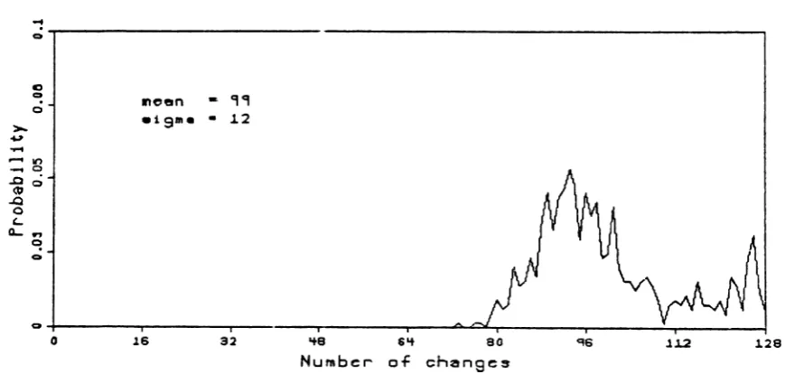
N. One approach could be to whiten the data thereby obtaining independent variables. This would, in part, involve the determination of eigenvalues and eigenvectors for an NxN covariance matrix. Due to the. complexity of this problem, the clustering effect is determined using the same probability measure, but the probabilities are produced by actually finding histograms from synthetically generated images. These histograms are compared with those from actual image sequences for visual similarity and agreement in mean and variance. In addition, chi square tests were performed. For these tests, the hypothesis that the values came from the same distribution could not be rejected at commonly accepted confidence levels.

3.3.4.2. Clustering results of mask generation

In order to obtain the most correct measure of the clustering, it would be necessary to count the changes in every possible block of size N. This is not only a computational burden, but it also is unnecessary in light of the block coding method used. Instead, the frames for the model images and the actual image were segmented into size N blocks with fixed length sides, in this case N=8x16, giving 640 blocks to use for the histogram. This sampling strategy is in exact agreement with the blocking used by the coder.

There are two mask types employed here to establish the clustering effect of the difference picture masks, and these correspond to whether a zero or nonzero threshold is used in order to determine the change status of a pixel. The first mask type includes any nonzero pixel in the difference frame as a valid change, and would indicate agreement in the statistics between the model and actual sequences regardless of how motion is determined. This then will include all changes due to noise as well as motion. The second mask type uses the a non-zero threshold of 3 which should include, for the most part, motion only changes. This method corresponds more to the clustering which would be encountered by the coder. Both methods are discussed beginning with the zero threshold.

1.1.4.2.1. Zero threshold elustering

56

Table 3.3: Synthetic image covariances.

[k' ,I') (0,0) (0,1) (1,0) (1,1) G1 1.000 0.953 0.955 0.911 G2 1.000 0.904 0.907 0.820 G3 1.000 0.852 0.856 0.730 G4 1.000 0.989 0.991 0.979

Figure 3.9 shows the zero threshold clustering distribution of the masks generated by three difference frames of BOBSJOB representing 12.3%, 18.1 %, and 25.3% motion as determined earlier in the chapter (clustering for the MAP sequence is similar). Note the bimodal shape and the fact that the right hand tail tends to stay up, particularly for the higher motion. The bimodal shape is due to the distri-bution being a combination of the clustering due to noise as well as that due to motion each with a difference mean. As an aside, the density for the number of changes was derived for the case of independent pixel intensities. Recall that this assumption was rejected earlier in the chapter. The density derived looked remarkably similar to the ones generated here and the cause of the bimodal shape could be easily determined from the density formula.

~

- - - ,

o

.128 .1.12

~e 6~ eo

Number of cnanscs

32

Incen - 96

.1S•• - 10

16

o

o ...

---...,.",Q".---...

---,---....--~~~f__---_,...----.,._---.-.

>-oU' ?'1 ..-. If) "'"'1 0 ~o ~ o '-CL- n ~ o

Figure 3.9a: Actual image clustering, motion=12.3%, threshold=O.

~

o ~---'---.,

Incen - 99 .1S.... • 12

C) Q o >-oU'

....

.... an .-. 0 ~o ..Q o c, CL- n ~ o Q -;---,---r---,r---~--g"..".:;..¥.._r__---__r_---~_r_---l

o 16 32 ~e 6~ 80

Number of cnanscs

J.12 .128

67

~

o~---'+8 S'+

Number 01=

32

mcen • 103

.is....

13

.16 o

Q-+- ----~---___,,._.:=~--__r_-oQ,,,,,.~~1__---__r_----r__---_1 GO

o

o

>.. ~ ...

--. .,., ... 0

-gO

.Q o '-a...,

C!

Q

:;

...

---,

o-.P---.---...----...,.-Incen .. 102

.i9•• - 8

.,

Q Q ... an .... Q ~Q ..Q o c, a..., C! o

o .16 32 ~8 6~ 80

Number of ch~nges

1J.2 ~28

Figure 3.10a: Gl clustering, motion=18.1 %, threshold=O.

~

o-r---~

0-+0---.---..---...

Inc!lIn - 101 .i9•• • 1 C Q Q >.. ~

....

:::8

~o ..Q o '-a... " C! o

o J6 32 ~e 6~ 80

Nu~ber of ch~nges

.1.1.2 J.29

59

~

0'---.128

~8 6~ eo

Number of cnangcs

32

lIleen • 101

.19m. - 6

lS

o

Q ~----,---r---r---~----9-~.L..--

...

---:::J.~-I

>-~ "?"'1 r-. .., ... c

-go

.Q o '-Q.. _n ~ Q

Figure 3.10c: G3 clustering, motion=18.1%,threshold=O.

.1

~

C).'"TI--- Q~---..----...----~-to

C)

o

>-. ~ ... ~It') ... 0

-go

.Q o '-Q.. n C! o o

Ilcen - 101

ei9rn. - 11

lS ~8 6~ 80

Number of changcs

.128

were truncated to integers and all nonzero values were counted as changes. The mean and variance are in fair agreement with the actual images and the tails tend to stay up, especially for the higher values of a₁ and a2. The bimodal shape, how-ever, is not present except for image G4 and it is not as pronounced as it is for the actual image with the same amount of motion. A13 an aside, note that there is a higher percentage of changed pixels in the synthetic image than in the actual. This may very well indicate that the noise variance as calculated is too high. The lack of a bimodal shape may also be due to the fact that the correlation in the synthetic masks may be too low. It may be informative to check both of these possibilities at this time beginning with the correlation.

61

Table 3.4: Zero threshold mask correlation with 18.1

%

motion.

(k' ,1') (0,0) (0,1 ) (1,0) (1,1) BOBSJOB 1.000 0.796 0.796 0.796

Gl 1.000 0.812 0.810 0.810

G2 1.000 0.807 0.807 0.806

G3 1.000 0.804 0.804 0.800

G4 1.000 0.811 0.810 0.810

In order to produce a more bimodal shape, higher values for a1 and a2 could

be tried. This was done with these parameters set to .999 for each. A problem was uncovered in that· the statistics for images of the size used here with these high correlation values were very good. In particular, the mean and variance were not close to the desired and the high correlation

was

not achieved.

The second possibility for the lack of bimodal shape may be due to the fact that the noise variance used is too large as was stated above. This means that the motion percentages are too low if the same amount of change is to be preserved between frames.

~---,

o

meen • 101

.1sm. -

10

o.J---.,..---.,...----r---+---,---,---1

o «) o >-~

....

... If)

. - . 0

-go

.Q o '-0..., ~ o

o 16 32 ~8 6~ eo

Number of cnanscs

.1J.2 ~2e

Figure 3.1Ia: GI clustering, rnotion=22.1

%,

threshold=O.

...

Q - - - ,

C) o

o

>-. ~

....

... If) .-. 0

-go

..Q o '-0..., ~ Q o

neen - 103 .1S•• - 13

.16 _.1.12

83

given in table 3.5 The clustering for the mask from G1is still not as good as for G4 with 18.1

%

motion. The clustering for G4 is somewhat better than it was before the motion percentage adjustment, however, the mask correlation values are not significantly changed. Given this lack of improvement by increasing the motion, the motion percen tages, as calculated, will be retained for now. In fact, the next section uses a non-zero threshold and suggests that motion may be overestimated.

Table 3.5: Zero threshold mask correlation with motion correction.

(k',1') (0,0) (0,1) (1,0) (1,1)

Gl 1.000 0.807 0.807 0.805

G4 1.000 0.808 0.806 0.807

The model, then, seems to be able to produce reasonably good agreement in zero threshold clustering if appropriate correlations are used, such as for image G4, and if motion percentages are assumed in the usual way, i.e., all magnitude changes greater than 3. It is clear that better statistics are needed for the noise and motion for the actual sequences. The next question to be addressed is that of the clustering effect of the model using a magnitude threshold of 3.

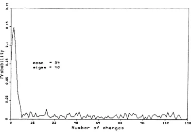
1.1.4.2.2. Non-aero threshold elustering

BOBSJOB frames. As may well be expected, the mean is much lower and the entire distribution is skewed to the left. Correlation values of the masks produced by an actual image are given in table 3.6 (the row labeled G4 corrected will be explained shortly).

Table 3.6: Non-zero threshold mask correlation with 18.1

%

motion.

(k' ,I') (0,0) (0,1 ) (1,0) (1,1) BOBS JOB 1.000 0.746 0.711 0.688

G1 1.000 0.787 0.787 0.705

G4 1.000 0.878 00879 0.831

G4 corrected 1.000 0.684 0.683 0.646

65 In

-0-m---.

n ~ Q .... c ... Q

..co

CD .c o '-Q..1t') Q Q

lnC'en - 11 .i9•• - 25

.128

J..1.2

32

J.6 ~8 6~ eo

Number of ch~nges

Figure 3.12a: Actual image clustering, motion=12.3%, threshold=3.

o

~

o-Tf"'1'---_... C)_Q

.co CD .c o '-Q..." Q Q

I"Icen • 25

.19•• • 35

.128 - J.L2

32

J8

o ~8 8~ 80

Nu~ber of changes

\I")

-0---,

n

-4 o

Ilcen - 3't

etgae • 'to

o 16 32 ~8 6~ eo

Nu~bcr o~ ch~nses

lJ.2 .128

~

o

-yt--- - - - -

_

o 87 ... C) ... Q

..co

_a:J ...0 o c, 11..." Q Q

o 16 32 ~8 6~ 80

Nu~bcr of changes

.128 Figure 3.13a: Gl clustering, motion=18.1%, threshold=3.

~

o~---

...

n

.... Q

rneen • 30

.19". - ~2

-.. c - Q

..co

_CD ...0 o c, 11...,., o o

o .16 32 ~8 6~ 80

Number of changes

these regions are sure to overlap in places, these high noise changes could still alter

the histograms and the correlation values.

This hypothesis can be checked by accounting for the noise when determining

the motion percentage. Let Pn be the probability of a change greater than 3 due

to noise, PTn be the probability of changes greater than 3 due to motion (i.e., the

motion percent), and P

r

be the total probab