R E S E A R C H
Open Access
Adaptive example-based super-resolution using
kernel PCA with a novel classification approach
Takahiro Ogawa
*and Miki Haseyama
Abstract
An adaptive example-based super-resolution (SR) using kernel principal component analysis (PCA) with a novel classification approach is presented in this paper. In order to enable estimation of missing high-frequency components for each kind of texture in target low-resolution (LR) images, the proposed method performs clustering of high-resolution (HR) patches clipped from training HR imagesin advance. Based on two nonlinear eigenspaces, respectively, generated from HR patches and their corresponding low-frequency components in each cluster, an inverse map, which can estimate missing high-frequency components from only the known low-frequency components, is derived. Furthermore, by monitoring errors caused in the above estimation process, the proposed method enables adaptive selection of the optimal cluster for each target local patch, and this
corresponds to the novel classification approach in our method. Then, by combining the above two approaches, the proposed method can adaptively estimate the missing high-frequency components, and successful
reconstruction of the HR image is realized.
Keywords:Super-resolution, resolution enhancement, image enlargement, Kernel PCA, classification
1 Introduction
In the field of image processing, high-resolution images are needed for various fundamental applications such as surveillance, high-definition TV and medical image pro-cessing [1]. However, it is often difficult to capture images with sufficient high resolution (HR) from current image sensors. Thus, methodologies for increasing reso-lution levels are used to bridge the gap between demands of applications and the limitations of hardware; and such methodologies include image scaling, interpo-lation, zooming and enlargement.
Traditionally, nearest neighbor, bilinear, bicubic [2], and sinc [3] (Lanczos) approaches have been utilized for enhancing spatial resolutions of low-resolution (LR) images. However, since they do not estimate high-fre-quency components missed from the original HR images, their results suffer from some blurring. In order to overcome this difficulty, many researchers have pro-posed super-resolution (SR) methods for estimating the missing high-frequency components, and this enhance-ment technique has recently been one of the most active
research areas [1,4-7]. Super-resolution refers to the task which generates an HR image from one or more LR images by estimating the high-frequency components while minimizing the effects of aliasing, blurring, and noise. Generally, SR methods are divided into two cate-gories: reconstruction-based and learning-based (exam-ple-based) approaches [7,8]. The reconstruction-based approach tries to recover the HR image from observed multiple LR images. Numerous SR reconstruction meth-ods have been proposed in the literature, and Park et al. provided a good review of them [1]. Most reconstruc-tion-based methods perform registration between LR images based on their motions, followed by restoration for blur and noise removal. On the other hand, in the learning-based approach, the HR image is recovered by utilizing several other images as training data. These motion-free techniques have been adopted by many researchers, and a number of learning-based SR meth-ods have been proposed [9-18]. For example, Freeman et al. proposed example-based SR methods that estimate missing high-frequency components from mid-frequency components of a target image based on Markov net-works and provide an HR image [10,11]. In this paper, we focus on the learning-based SR approach. * Correspondence: [email protected]
Graduate School of Information Science and Technology, Hokkaido University, Sapporo, Japan
Conventionally, learning-based SR methods using princi-pal component analysis (PCA) have been proposed for face hallucination [19]. Furthermore, by applying kernel methods to the PCA, Chakrabarti et al. improved the performance of the face hallucination [20] based on the Kernel PCA (KPCA; [21,22]). Most of these techniques are based on global approaches in the sense that proces-sing is done on the whole of LR images simultaneously. This imposes the constraint that all of the training images should be globally similar, i.e., they should repre-sent a similar class of objects [7,23,24]. Therefore, the global approach is suitable for images of a particular class such as face images and fingerprint images. How-ever, since the global approach requires the assumption that all of the training images are in the same class, it is difficult to apply it to arbitrary images.
As a solution to the above problem, several methods based on local approaches in which processing is done for each local patch within target images have recently been proposed [13,25,26]. Kim et al. developed a global-based face hallucination method and a local-global-based SR method of general images by using the KPCA [27]. It should be noted that even if the PCA or KPCA is used in the local approaches, all of the training local patches are not necessarily in the same class, and their eigen-space tends not to be obtained accurately. In addition, Kanemura et al. proposed a framework for expanding a given image based on an interpolator which is trained in advance with training data by using sparse Bayesian esti-mation [12]. This method is not based on PCA and KPCA, but calculates the Bayes-based interpolator to obtain HR images. In this method, one interpolator is estimated for expanding a target image, and thus, the image should also contain only the same kind of class. Then it is desirable that training local patches are first clustered and the SR is performed for each target local patch using the optimal cluster. Hu et al. adopted the above scheme to realize the reconstruction of HR local patches based on nonlinear eigenspaces obtained from clusters of training local patches by the KPCA [8]. Furthermore, we have also proposed a method for reconstructing missing intensities based on a new classi-fication scheme [28]. This method performs the super-resolution by treating this problem as a missing intensity interpolation problem. Specifically, our previous method introduces two constraints, eigenspaces of HR patches and known intensities, and the iterative projection onto these constraints is performed to estimate HR images based on the interpolation of the missing intensities removed by the subsampling process. Thus, in our pre-vious work, intensities of a target LR image are directly utilized as those of the enlarged result. Thus, if the tar-get LR image is obtained by blurring and subsampling
its HR image, the intensities in the estimated HR image contain errors.
In conventional SR methods using the PCA or KPCA, but not including our previous work [28], there have been two issues. First, it is assumed in these methods that the LR patches and their corresponding HR patches that are, respectively, projected onto linear or nonlinear eigenspaces are the same, these eigenspaces being obtained from training HR patches [8,27]. However, these two are generally different, and there is a tendency for this assumption not to be satisfied. Second, to select optimal training HR patches for target LR patches, dis-tances between their corresponding LR patches are only utilized.
Unfortunately, it is well known that the selected HR patches are not necessarily optimal for the target LR patches, and this problem is known as theoutlier pro-blem. This problem has also been reported by Datsenko and Elad [29,30].
In this paper, we present an adaptive example-based SR method using KPCA with a novel texture classifica-tion approach. The proposed method first performs the clustering of training HR patches and generates two nonlinear eigenspaces of HR patches and their corre-sponding low-frequency components belonging to each cluster by the KPCA.
minimum distance of the estimation result and the known parts of the target patch, and thus we adopt it as the new criterion. Consequently, by the inverse map determined from the nonlinear eigenspaces of the opti-mal cluster, the missing high-frequency components of the target patches are adaptively estimated. Therefore, successful performance of the SR can be expected. This paper is organized as follows: first, in Section 2, we briefly explain KPCA used in the proposed method. In Section 3, we discuss the formulation model of LR images. In Section 4, the adaptive KPCA-based SR algo-rithm is presented. In Section 5, the effectiveness of our method is verified by some results of experiments. Con-cluding remarks are presented in Section 6.
2 Kernel principal component analysis
In this section, we briefly explain KPCA used in the proposed method. KPCA was first introduced by Schölk-opf et al. [21,22], and it is a useful tool for analyzing data which contain nonlinear structures. Given target dataxi (i= 1, 2, . . . , N), they are first mapped into a feature space via a nonlinear map: φ:RM→F, where M is the dimension ofxi.Then we can obtain the data mapped into the feature space,j(x1), j(x2), . . . ,j(xN). For simplifying the following explanation, we assume these data are centered, i.e.,
N
i=1
φ(xi) = 0. (1)
For performing PCA, the covariance matrix
R= 1
N N
i=1
φ(xi)φ(xi) (2)
is calculated, and we have to find eigenvalues l and eigenvectorsuwhich satisfy
λu=Ru. (3)
In this paper, vector/matrix transpose in both input and feature spaces is denoted by the superscript‘.
Note that the eigenvectorsulie in the span ofj(x1),j (x2), . . . ,j(xN), and they can be represented as follows:
u=α, (4)
whereΞ= [j(x1),j(x2), . . . ,j(xN)] andais anN ×1 vector. Then Equation 3 can be rewritten as follows:
λα=Rα. (5)
Furthermore, by multiplyingΞ’by both sides, the fol-lowing equation can be obtained:
λα=Rα. (6)
Therefore, from Equation 2,Rcan be represented by
1
N
, and the above equation is rewritten as
NλKα=K2α, (7)
whereK=Ξ’Ξ. Finally,
Nλα=Kα, (8)
is obtained. By solving the above equation,a can be obtained, and the eigenvectorsu can be obtained from Equation 4.
Note that (i, j)th element of Kis obtained byj(xi)’j (xj). In kernel methods, it can be obtained by using ker-nel trick [21]. Specifically, it can be obtained by some kernel functions (xi, xj) using only xi and xj in the input space.
3 Formulation model of LR images
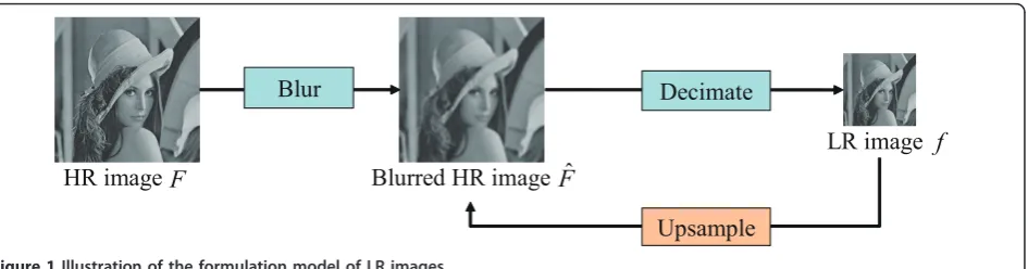
This section presents the formulation model of LR images in our method. In the common degradation model, an original HR image F is blurred and deci-mated, and the target LR image including the additive noise is obtained. Then, this degradation model is repre-sented as follows:
f=DBF+n, (9)
where f and F are, respectively, vectors whose ele-ments are the raster-scanned intensities in the LR image f and its corresponding HR image F. Therefore, the dimension of these vectors are, respectively, the number of pixels in fand F. D and B are the decimation and blur matrices, respectively. The vector nis the noise vector, whose dimension is the same as that off. In this paper, we assume that nis the zero vector in order to make the problem easier. Note that if decimation is per-formed without any blur, the observed LR image is severely aliased.
Generally, actual LR images captured from commer-cially available cameras tend to be taken without suffer-ing from aliassuffer-ing. Thus, we assume that such captured LR images do not contain any aliasing effects. However, it should be noted that for realizing the SR, we can con-sider several assumptions, and thus, we focus on the fol-lowing three cases:
Case 2: LR images are captured by only the decima-tion procedure without using any low-pass filters. In this case, some aliasing effects occur, and interpolation-based methods work better than our method.
Case 3 : LR images are captured based on the low-pass filter followed by the decimation procedure, but some aliasing effects occur. In this case, the problem becomes much more difficult than those of Cases 1 and 2. Furthermore, in our method, it becomes difficult to model this degradation process.
We focus only on Case 1 to realize the SR, but some comparisons between our method and the methods focusing on Case 2 are added in the experiments.
For the following explanation, we clarify the defini-tions of the following four images:
HR image F whose vector is F in Equation 9 is the original image that we try to estimate.
Blurred HR image Fˆ whose vector is BFis obtained by applying the low-pass filter to the HR image F. Its size is the same as that of the HR image.
LR image fwhose vector isf (=DBF) is obtained by applying the subsampling to the blurred HR image Fˆ.
High-frequency components whose vector is F - BF are obtained by subtractingBFfromF.
Note that the HR image, the blurred HR image, and the high-frequency components have the same size. In order to define the blurred HR image, the LR image, and the high-frequency components, we have to provide which kind of the low-pass filter is utilized for defining the matrixB. Generally, it is difficult to know the details of the low-pass filter and provide the knowledge of the blur matrix B. Therefore, we simply assume that the low-pass filter is fixed to the sinc filter with the ham-ming window in this paper. In the proposed method, high-frequency components of target images must be estimated from only their low-frequency components and other HR training images. This means when the high-frequency components are perfectly removed, the problem becomes the most difficult and useful for the performance verification. Since it is well known that the sinc filter is suitable one to effectively remove the high-frequency components, we adopted this filter. Further-more, the sinc filter has infinite length coefficients, and thus we also adopted the hamming window to truncate the filter coefficients. The details of the low-pass filter is shown in Section 5. Since the matrix Bis fixed, we dis-cuss the sensitivity of our method to the errors in the matrixBin Section 5.
In the proposed method, we assume that LR images are captured based on the low-pass filter followed by the decimation, and aliasing effects do not occur. Furthermore, the decimation matrix is only an operator which subsamples pixel values. Therefore, when the
magnification factor is determined for target LR images, the matrices B and D can be also obtained in our method. Specifically, the decimation matrixD can be easily defined when the magnification factor is deter-mined. In addition, the blurring matrixBis also defined by the sinc function with the hamming window in such a way that target LR images do not suffer from aliasing effects. In this way, the matrices B and D can be defined, but in our method, these matrices are not directly utilized for the reconstruction. The details are shown in the following section.
As shown in Figure 1, by upsampling the target LR image f, we can obtain the blurred HR image Fˆ. How-ever, it is difficult to reconstruct the original HR image Ffrom Fˆ since the high-frequency components ofFare missed by the blurring. Furthermore, the reconstruction of the HR image becomes more difficult with increase in the amount of blurring [7].
4 KPCA-based adaptive SR algorithm
An adaptive SR method based on the KPCA with a novel texture classification approach is presented in this section. Figure 2 shows an outline of our method. First, the proposed method clips local patches from training HR images and performs their clustering based on the KPCA. Then two nonlinear eigenspaces of the HR patches and their corresponding low-frequency compo-nents are, respectively, obtained for each cluster. Furthermore, the proposed method clips a local patch ˆg
In order to realize the adaptive SR algorithm, the training HR patches must first be assigned to several clusters before generating each cluster’s nonlinear eigen-spaces. Therefore, the clustering method is described in detail in 4.1, and the method for estimating the missing high-frequency components of the target local patches is presented in 4.2.
4.1 Clustering of training HR patches
In this subsection, clustering of training HR patches into Kclusters is described. In the proposed method, we cal-culate a nonlinear eigenspace for each cluster and enable the modeling of the elements belonging to each cluster by its nonlinear eigenspace. Then, based on these nonlinear eigenspaces, the proposed method can perform the clustering of training HR patches in this
subsection and the high-frequency component estima-tion, which simultaneously realizes the classification of target patches for realizing the adaptive reconstruction, in the following subsection. This subsection focuses on the clustering of training HR patches based on the non-linear eigenspaces.
From one or some training HR images, the proposed method clips local patchesgi (i= 1, 2, . . . , N;Nbeing the number of the clipped local patches), whose size is w × h pixels, at the same interval. Next, for each local patch, two images, gL
i and giH, which contain
low-fre-quency and high-frelow-fre-quency components of gi, respec-tively, are obtained. This means gi,gLi,gHi , respectively, correspond to local patches clipped from the same posi-tion of (a) HR image, (b) Blurred HR image, and (d)
F
ˆ
f
Blur
Decimate
HR image
Blurred HR image
LR image
F
Upsample
Figure 1Illustration of the formulation model of LR images.
HR image
F
Blurred HR imageF
ˆ
…
Cluster 1 Cluster 2 Cluster K
Training HR image
Clipped HR patchesgi(i=1,2,K,N)
Clustering algorithm of training HR patches
Estimation of missing high-frequency components Adaptive selection of the optimal cluster Target local
patch
g
ˆ
Estimated HR patch of g
Nonlinear eigenspace of HR patches in cluster k
Nonlinear eigenspace of corresponding low-frequency components in cluster k
high-frequency components shown in the previous sec-tion. Then the two vectors li andhi containing raster-scanned elements of gL
i and giH, respectively, are
calcu-lated. Furthermore,li is mapped into the feature space via a nonlinear map: φ:Rwh→F[22], where the non-linear map whose kernel function is the Gaussian kernel is utilized. Specifically, given two vectors a and b (Î Rwh
), the Gaussian kernel function in the proposed method is defined as follows:
κ(a, b) = exp
−||a−b||2 σ2
1
, (10)
where σ2
1 is a parameter of the Gaussian kernel. Then the following equation is satisfied:
φ(a)φ(b) =κ(a, b). (11)
Then a new vector ji = [j(li)’, hi’]’is defined. Note that an exact pre-image, which is the inverse mapping from the feature space back to the input space, typically does not exist [31]. Therefore, the estimated pre-image includes some errors. Since the final results estimated in the proposed method are the missing high-frequency components, we do not utilize the nonlinear map forhi (i= 1, 2, . . . ,N).
From the obtained results ji (i = 1, 2, . . . , N), the proposed method performs clustering that minimizes the following criterion:
C= K k=1 Nk j=1
||lkj − ˜lkj||2+||hkj − ˜h k
j||2, (12)
where Nk is the number of elements belonging to cluster k. Generally, superscript is used to indicate the power of a number. However, in this paper, onlykdoes not represent the power of a number. The vectors lkj
and hkj (j= 1, 2, . . . ,Nk), respectively, represent liand hiofgi(i= 1, 2, . . . ,N) assigned to clusterk. In Equa-tion 12, the proposed method minimizesCwith respect to the belonging cluster number of each local patchgi. Each known local patch belongs to the cluster whose nonlinear eigenspace can perform the most accurate approximation of its low- and high-frequency compo-nents. Therefore, using Equation 12, we try to determine the clustering results, i.e., which cluster is the optimal for each known local patchgi.
Note that in Equation 12, ˜lkj and h˜kj in the input
space are, respectively, the results projected onto the nonlinear eigenspace of clusterk. Then, in order to cal-culate them, we must first obtain the projection result
˜ φk
j onto the nonlinear eigenspace of clusterkfor each
φk
j = [φ(l
k
j), hkj]. Furthermore, when φjk= [φ(l k
j), hkj]
is defined and its projection result onto the nonlinear eigenspace of clusterkis defined as φ˜jk in the feature space, the following equation is satisfied:
˜ φk
j =UkUk
φk
j − ¯φk
+φ¯k, (13)
whereUkis an eigenvector matrix of clusterk, and φ¯k
is the mean vector of φkj (j = 1, 2, . . . , Nk) and is obtained by
¯ φk= 1
Nk
kek. (14)
In the above equation,ek= [1, 1, . . . , 1]’is anNk×1 vector. As described above, φ˜kj is the projection result
of φjk onto the nonlinear eigenspace of cluster k, i.e.,
the approximation result of φkj in the subspace of clus-ter k. Therefore, Equation 13 represents the projection of j-th element of cluster konto the nonlinear eigen-space of cluster k. Note that from Equation 13, φ˜k
j can
be defined as φ˜k
j = [ζk
j , h˜
k
j ]. In detail, ζ k
j corresponds
to the projection result of the low-frequency
compo-nents in the feature space. Furthermore, h˜kj corresponds
to the result of the high-frequency components, and it
can be obtained directly. However, ˜lkj in Equation 12
cannot be directly obtained since the projection result ζk
j is in the feature space. Generally, we have to solve
the pre-image estimation problem of ˜lkj from ζjk, i.e.,
˜
lkj, which satisfies ζk
j ∼= φ(˜l
k
j), has to be estimated. In
this paper, we call this pre-image approximation as [Approximation 1] for the following explanation.
Gener-ally, if we perform the pre-image estimation of ˜lkj from
ζk
j , estimation errors occur. In the proposed method,
we adopt some useful derivations in the following
expla-nation and enable the calculation of ||lkj − ˜lkj||2 in
Equa-tion 12 without directly solving the pre-image problem of ζjk.
In the above equation,
Uk= [uk1,uk2,. . .,ukDk] (D
k<Nk) (15)
Th. The value Th is a threshold to determine the dimension of the nonlinear eigenspaces from its cumu-lative proportion. Furthermore, k= [φk
1, φ2k, . . ., φNkk] andHkis a centering matrix defined as follows:
Hk=Ek− 1
Nke
kek, (16)
whereEkis theNk× Nkidentity matrix. The matrixH plays the centralizing role, and it is commonly used in general PCA and KPCA-based methods.
In Equation 15, the eigenvectors uk
d(d= 1, 2, . . ., Dk)
are infinite-dimensional since uk
d(d= 1, 2, . . ., Dk) are
eigenvectors of the vectors φkj (j= 1, 2, . . ., Nk) with the infinite dimension. This means that the dimension of the eigenvectors must be the same as that of φjk.
Then since φk
j is infinite dimensional, the dimension of
ukd is also infinite. It should be noted that since there
areDkeigenvectors uk
d(d= 1, 2, . . ., Dk), theseD
k vec-tors span the nonlinear eigenspace of clusterk. From the above reason, Equation 13, therefore, cannot be cal-culated directly. Thus, we introduce the computational scheme, kernel trick, into the calculation of Equation 13. The eigenvector matrixUk satisfies the following singu-lar value decomposition:
k
Hk∼= UkkVk, (17)
whereΛkis the eigenvalue matrix andVkis the eigen-vector matrix of HkΞk’ΞkHk. Therefore, Uk can be obtained as follows:
Uk∼= kHkVkk−1. (18)
As described above, the approximation of the matrix Uk
is performed. This is a common scheme in KPCA-based methods, where we call this approximation [Approximation 2], hereafter. Since the columns of the matrixUkare infinite-dimensional, we cannot directly use this matrix for the projection onto the nonlinear eigenspace. Therefore, to solve this problem, the matrix Uk
is approximated by Equation 18 for realizing the ker-nel trick. Note that if Dk becomes the same as the rank of Ξk, the approximation in Equation 18 becomes equivalent relationship.
From Equations 14 and 18, Equation 13 can be rewrit-ten as
˜ φk
j ∼=kHkVkk
−2 VkHkk
φk j −
1 Nk
kek
+ 1 Nk
kek
=kWkk
φk j −
1 Nk
kek
+ 1 Nk
kek,
(19)
where
Wk=HkVkk−2VkHk. (20)
Next, since we utilize the nonlinear map of the
Gaus-sian kernel, ||lkj − ˜lkj||2 in Equation 12 satisfies
φ(lkj)φ(˜lkj) = exp
⎧ ⎨
⎩−
||lkj − ˜l
k j||2
σ2 1
⎫ ⎬ ⎭
∼= φ(lkj)ζjk.
(21)
Furthermore, given k
l = [φ(l
k
1), φ(lk2). . ., φ(lkNk)]
and k
h = [h
k
1, h
k
2, . . ., h
k
Nk], they satisfy
k= [k
l ,
k
h]. Thus, from Equation 19, ζ
k
j in
Equa-tion 21 is obtained as follows:
ζk
j ∼= klW
kk
φk
j −
1
Nk
kek
+ 1 Nk k le k. (22)
Then, by using Equations 21 and 22, ||lkj − ˜lkj||2 in
Equation 12 can be obtained as follows:
||lk j− ˜l
k j||2=−σ12log
φ(lk
j)φ(˜l k j)
∼=−σ12log
φ(lk j)ζjk
∼=−σ2 1log
φ(lk
j)klW
kk
φk
j−
1 Nk
kek
+ 1
Nkφ(l k j)kle
k
.
(23)
Furthermore, since h˜kj is calculated from Equation 19
as
˜
hkj ∼= khWkk
φk
j −
1
Nk
kek
+ 1
Nk
k
hek, (24)
||hkj− ˜hkj||2 in Equation 12 is also obtained as follows:
||hkj− ˜h k j||2∼=
hkj−khW
kk
φk j−
1
Nk
kek − 1 Nk k he k 2 . (25)
Then, from Equations 23 and 25, the criterion C in Equation 12 can be calculated. It should be noted that for calculating the criterion C, we, respectively, use Approximations 1 and 2 once through Equations 21-25.
In Equation 13,Ukis utilized for the projection onto the eigenspace spanned by their eigenvectors ukd(d= 1, 2, . . ., Dk). Therefore, the criterionC repre-sents the sum of the approximation errors of
φk
j (j= 1, 2, . . ., Nk) in their eigenspaces. This means
that the squared error in Equation 12 corresponds to the distance from the nonlinear eigenspace of each cluster in the input space. Then, the new criterionCis useful for the clustering of training HR local patches. From the cluster-ing results, we can obtain the eigenvector matrixUk
φk
j (j= 1, 2, . . ., Nk) belonging to cluster k.
Further-more, we define φˆkj = [φ(lkj), 0’](j= 1, 2, . . ., Nk)and
also calculate the eigenvector matrix Uˆk for ˆ
φk
j (j= 1, 2, . . ., Nk) belonging to clusterk. Finally, we
can, respectively, obtain the two nonlinear eigenspaces of HR training patches and their corresponding low-fre-quency components for each clusterk.
4.2 Adaptive estimation of missing high-frequency components
In this subsection, we present an adaptive estimation of missing high-frequency components based on the KPCA. We, respectively, define the vectors of gand ˆg
asj* = [j(l)’, h’]’ and φˆ= [φ(l), 0’] in the same way as jiand φˆi. From the above definitions, the following
equation is satisfied:
ˆ φ=
EDφ×Dφ ODφ×wh
Owh×Dφ Owh×wh
φ∗ = φ∗,
(26)
whereEp × qandOp × qare, respectively, the identity matrix and the zero matrix whose sizes arep × q. Further-more,Djrepresents the dimension of the feature space, i.
e., infinite dimension in our method. The matrix EDφ×Dφ
is the identity matrix whose dimension is the same as that ofj(l) and Owh × whrepresents the zero matrix which removes the high-frequency components. As shown in the previous section, our method assumes that LR images are obtained by removing their high-frequency components, and aliasing effects do not occur. This means our problem is to estimate the perfectly removed high-frequency com-ponents from the known low-frequency comcom-ponents. Therefore, the problem shown in this section is equivalent to Equation 9, and the solution that is consistent with Equation 9 can be obtained.
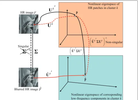
In Equation 26, since the matrixΣ is singular, we can-not directly calculate its inverse matrix to estimate the missing high-frequency componentsh and obtain the original HR image. Thus, the proposed method, respec-tively, mapsj*and φˆ onto the nonlinear eigenspace of HR patches and that of their low-frequency components in clusterk. Furthermore, the projection corresponding to the inverse matrix ofΣ is derived in these subspaces. We show its specific algorithm in the rest of this sub-section and its overview is shown in Figure 3.
First, the vector j* is projected onto the Dk -dimen-sional nonlinear eigenspace of cluster kby using the eigenvector matrixUkas follows:
p=Uk(φ∗− ¯φk). (27)
Furthermore, the vector φˆ is also projected onto the Dk-dimensional nonlinear eigenspace of cluster k by using the eigenvector matrix Uˆk as follows:
ˆ
p=Uˆkφˆ− ˜φk, (28)
where φ˜k is defined as
˜ φk= 1
Nkˆ k
ek, (29)
and ˆk= [φˆk
1,φˆ2k, . . .,φˆkNk]. Furthermore, j* is approximately calculated as follows:
φ∗∼= Ukp+φ¯k. (30)
In the above equation, the vector of the original HR patch is approximated in the nonlinear eigenspace of clusterk, where we call this approximation [Approxima-tion 3]. The nonlinear eigenspace of cluster kcan per-form the least-square approximation of its belonging elements. Therefore, if the target local patch belongs to clusterk, accurate approximation can be realized. Then the proposed method introduces the classification pro-cedures for determining which cluster includes the tar-get local patch in the following explanation. Next, by substituting Equations 26 and 30 into Equation 28, the following equation is obtained:
ˆ p∼= Uˆk
Ukp+φ¯k
− ˆUk
˜ φk . (31) Thus, ˆ
UkUkp∼= pˆ− ˆUkφ¯k+Uˆkφ˜k
=pˆ (32)
since
˜ φk
=φ¯k. (33)
The vector φ˜k corresponds to the mean vector of the
vectors φˆjk whose high-frequency components are
removed from φk
j (j= 1, 2, . . ., Nk). Then
˜ φk= 1
Nkˆ k
ek
= 1
Nk
kek
=
1
Nk
kek
= φ¯k
(34)
is derived, where ˆk= [φˆk
In Equation 32, if the rank ofΣ is larger thanDk, the matrix Uˆk
Ukbecomes a non-singular matrix, and its inverse matrix UˆkUk−1 80can be calculated. In
detail, the rank of the matrices Uˆk and Uk is Dk. Although the rank ofΣ is not full and its inverse matrix cannot be directly obtained, the rank of Uˆk
Uk becomes min (Dk, rank(Σ)). Therefore, if rank(Σ)≥ Dk, ˆ Uk Uk −1
can be calculated. Then
p∼=
ˆ
UkUk− 1
ˆ
p. (35)
Finally, by substituting Equations 27 and 28 into the above equation, the following equation can be obtained:
Uk(φ∗− ¯φk)∼=
ˆ
UkUk− 1
ˆ
Ukφˆ− ˜φk. (36)
Then we can calculate an approximation result
φk
=φk
1
,hk
of j* from cluster k’s eigenspace as
follows:
φk=UkUˆkUk−1Uˆkφˆ− ˜φk+φ¯k. (37)
Furthermore, in the same way as Equation 19, we can obtain the following equation:
φk∼
= kTkˆkφˆ−φ¯k+φ¯k, (38)
whereTkis calculated as follows:
Tk=HkVk(Vˆk
Hkˆk
k
HkVk)−1Vˆk
Hk (39)
and Vˆk is an eigenvector matrix ofˆk
HkHkˆk. Note that the estimation result, which we have to estimate, is
HR image
F
F
ˆ
Blurred HR image
Nonlinear eigenspace of
HR patches in cluster
k
Nonlinear eigenspace of corresponding
low-frequency components in cluster
k
Σ
1
−
Σ
1ˆ
⎟
−⎠
⎞
⎜
⎝
⎛ ′
U
kΣU
k⎟
⎠
⎞
⎜
⎝
⎛ ′
U
ˆ
kΣU
k′
kU
′
kU
ˆ
kU
Singular
Non-singular
p
p
ˆ
the vector h of the unknown high-frequency compo-nents. Since Equation 38 is rewritten as
φk
l
hk
∼= kl
k
h
Tkklφ(l)− ¯φk1+
¯ φk l ¯ hk , (40)
whereφ¯k=φ¯k
l ,h¯
k
. Thus, from Equations 14 and 40, the vector hk, which is the estimation result of hby clusterk, is calculated as follows:
hk∼= khTkk l
φ(l)− 1
Nk
k
lek
+ 1
Nk
k
hek. (41)
Then, by utilizing the nonlinear eigenspace of cluster k, the proposed method can estimate the missing high-frequency components. In this scheme, we, respectively, use Approximations 2 and 3 once through Equations 31-41.
The proposed method enables the calculation of the inverse map which can directly reconstruct the high-fre-quency components. In the previously reported methods [8,27], they simply project the known frequency compo-nents to the eigenspaces of the HR patches, and their schemes do not correspond to the estimation of the missing high-frequency components. Thus, these meth-ods do not always provide the optimal solutions. On the other hand, the proposed method can provide the opti-mal estimation results if the target local patches can be represented in the obtained eigenspaces, correctly. This is the biggest difference between our method and the conventional methods.
Furthermore, we analyze our method in detail as follows.
It is well-known that the elements φjk of
gkj (j= 1, 2, . . ., Nk), which aregibelonging to cluster k, can be correctly approximated in their nonlinear eigenspace in the least-squares sense. Therefore, if we can appropriately classify the target local patch into the optimal cluster from only the known parts gˆ, the pro-posed method successfully estimates the missing high-frequency components h by its nonlinear eigenspace. Unfortunately, if we directly utilize gˆ for selecting the optimal cluster, it might be impossible to avoid the out-lier problem. Thus, in order to achieve classification of the target local patch without suffering from this pro-blem, the proposed method utilizes the following novel criterion as a substitute for Equation 12:
˜
Ck= ||l−lk||2, (42)
where lkis a pre-image of φk
l . In the above equation,
since we utilize the nonlinear map of the Gaussian
kernel, ||l-lk||2is satisfied as follows:
φ(l)φ(lk) = exp
−||l−lk||2 σ2
l
∼=φ(l)φlk,
(43)
and φk
l is calculated from Equations 14 and 40 below.
φk
l ∼= klTkk
l
φ(l)− 1
Nk
k
lek
+ 1
Nk
k
lek. (44)
Then, from Equations 43 and 44, the criterion C˜k in
Equation 42 can be rewritten as follows:
˜
Ck∼
=−σl2log
φ(l)k lTkk
l
φ(l)− 1
Nk
k lek
+ 1
Nkφ(l)
k lek
. (45)
In this derivation, Approximation 1 is used once. The criterion C˜k represents the squared error calculated
between the low-frequency componentslkreconstructed with the high-frequency components hk by cluster k’s nonlinear eigenspace and the known original low-fre-quency componentsl.
We introduce the new criterion into the classification of the target local patch as shown in Equations 42 and 45. Equations 42 and 45 utilized in the proposed method represent the errors of the low-frequency com-ponents reconstructed with the high-frequency compo-nents by Equation 40. In the proposed method, if both of the target low-frequency and high-frequency compo-nents are perfectly represented by the nonlinear eigen-spaces of cluster k, the approximation relationship in Equation 32 becomes the equal relationship. Therefore, if we can ignore the approximation in Equation 38, the original HR patches can be reconstructed perfectly. In such a case, the errors caused in the low-frequency and high-frequency components become zero. However, if we apply the proposed method to general images, the target low-frequency and high-frequency components cannot perfectly be represented by the nonlinear eigen-spaces of one cluster, and the errors are caused in those two components. Specifically, the caused errors are obtained as
˜
Cktrue= ||l−lk||2+||h−hk||2 (46)
= 0 and calculate the minimum errors C˜k of C˜k
true. This means the proposed method utilizes the minimum errors caused in the HR result estimated by the inverse projection which can optimally provide the original image for the elements of each cluster. Then the pro-posed method utilizes the error C˜k in Equation 45 as
the criterion for the classification. In the previously reported method based on KPCA [8], they only applied the simplek-means method to the known low-frequency components for the clustering and the classification. Thus, this approach is quite independent of the KPCA-based reconstruction scheme, and there is no guarantee of providing the optimal clustering and classification results. On the other hand, the proposed method derives all of the criteria for the clustering and the classification from the KPCA-based reconstruction scheme. There-fore, it can be expected that this difference between the previously reported method and our method provides a solution to the outlier problem.
From the above explanation, we can see C˜k in
Equa-tion 45 is a suitable criterion for classifying the target local patch into the optimal clusterkopt. Then, the pro-posed method regards hkopt estimated by the selected clusterkoptas the output, and l+hkopt
becomes the esti-mated vector of the target HR patchg.
As described above, it becomes feasible to reconstruct the HR patches from the optimal cluster in the pro-posed method. Finally, we clip local patches (w × h pix-els) at the same interval (w˜ × ˜hpixels) from the blurred HR image Fˆ and reconstruct their corresponding HR patches. Note that each pixel has multiple reconstruc-tion results if the clipping interval is smaller than the size of the local patches. In such a case, the proposed method outputs the result minimizing Equation 45 as the final result. Then, the adaptive SR can be realized by the proposed method.
5 Experimental results
In this section, we verify the performance of the pro-posed method. As shown in Figures 4a, 5a, and 6a, we prepared three test images Lena, Peppers, and Goldhill utilized in many papers. In order to obtain their LR images shown in Figures 4b, 5b, and 6b, we subsampled them to quarter size by using the sinc filter with the hamming window. Specifically, the filterw(m, n) of size (2L+ 1) × (2L+ 1) is defined as
w(m,n) =0.54 + 0.46cosπm
L 0.54 + 0.46cos
πn
L
sinπm s
πm
sinπn s
πn
(|m| ≤L,|n| ≤L), (47)
wheres corresponds to the magnification factor, and we setL = 12. In these figures, we simply enlarged the LR images to the size of the original images. When we
estimate an HR result from its LR image, the other two HR images and Boat, Girl, Mandrill are utilized as the training data. In the proposed method, we simply set its parameters as follows:w = 8,h= 8, w˜ = 8, h˜= 8, Th = 0.9, σ2
l is 0.075 times the variance of ||li -lj||2 (i, j = 1, 2, . . . ,N), andK= 7. Note that the parameters σl2 and K seem to affect the performance of the proposed method. Thus, we discuss the determinations of these two parameters and their sensitivities in Appendix. In this experiment, we applied the previously reported methods and the proposed method to Lena, Peppers, and Goldhill and obtained their HR results, where the magnification factor was set to four. For comparison, we adopt the method utilizing the sinc interpolation, which is the same filter used in the downsampling process and the most traditional approach, and three previously reported methods [8,11,27]. Since the method in [11] is a representative method of the example-based super-resolution, we utilized this method in the experiment. Furthermore, the method [27] is also a representative method which utilizes KPCA for performing the super-resolution, and its improvement is achieved by utilizing the classification scheme in [8]. Therefore, these two methods are suitable for the comparison to verify the proposed KPCA-based method including the novel clas-sification approach. In addition, the methods in [12,28] have been proposed for realizing accurate SR. Therefore, since these methods can be regarded as state-of-the-art ones, we also adopted them for comparison of the pro-posed method.
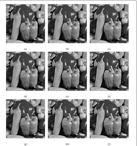
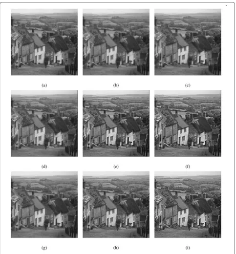
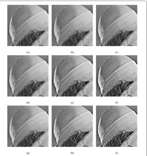
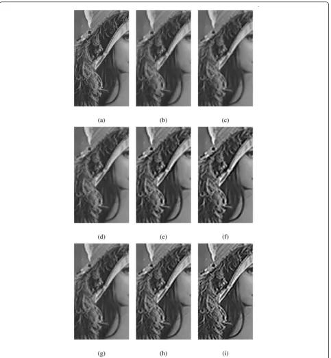
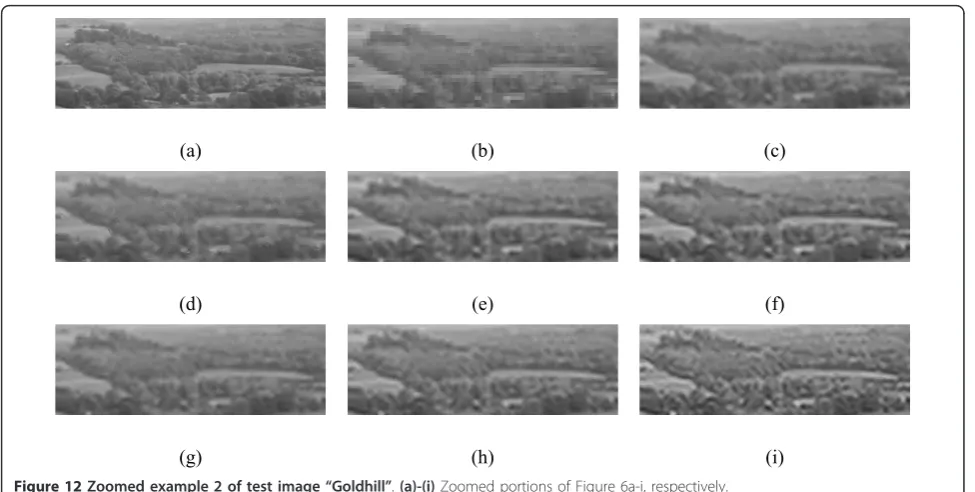
First, we focus on test image Lena shown in Figure 4. We, respectively, show the HR images estimated by the sinc interpolation, the previously reported methods [8,11,12,27,28], and the proposed method in Figures 4c-i. In the experiments, the HR images estimated by both of the conventional methods and the proposed method were simply high-boost filtered for better comparison as shown in [27]. From the zoomed portions shown in Fig-ures 7 and 8, we can see that the proposed method pre-serves the sharpness more successfully than do the previously reported methods. Furthermore, from the other two results shown in Figures 5, 6, and 9, 10, 11, 12, we can see various kinds of images are successfully reconstructed by our method. As shown in Figures 4, 5, 6, 7, 8, 9, 10, 11, 12, Goldhill contains more high-fre-quency components than the other two test images Lena and Peppers. Therefore, the difference of the per-formance between the previously reported methods and the proposed method becomes significant.
edge regions of test image Lena as shown in Figure 7. Furthermore, in the texture regions which are shown in Figure 8, the difference between the proposed method
and the other methods becomes significant. Further-more, in Figures 9 and 10, the center regions contain more high-frequency components compared with the
(a) (b) (c)
(d) (e) (f)
(g) (h) (i)
Figure 4Comparison of results (Test image“Lena”, 512 × 512 pixels) obtained by using different image enlargement methods.(a)
Original HR image.(b)LR image of(a). HR image reconstructed by (c) sinc interpolation,(d)reference [11],(e)reference [27],(f)reference [8],
other regions. Thus, the proposed method successfully reconstructs sharp edges and textures. As described above, test image Goldhill contains more high-frequency components than the other two test images, the differ-ence of our method and the other ones is quite signifi-cant. Particularly, in Figure 11, roofs and windows can
be successfully reconstructed with keeping sharpness by the proposed method. In addition, in Figure 12, the whole areas can be also accurately enhanced.
Some previously reported methods such as [12,27] estimate one model for performing the SR. Then, if var-ious kinds of training images are provided, it becomes
Figure 5Comparison of results (Test image“Peppers”, 512 × 512 pixels) obtained by using different image enlargement methods.(a)
Original HR image.(b)LR image of(a). HR image reconstructed by(c)sinc interpolation,(d)reference [11],(e)reference [27],(f)reference [8],
difficult to successfully estimate the high-frequency components, and the obtained results tend to be blurred. Thus, we have to perform clustering of training patches in advance and reconstruct the high-frequency components by the optimal cluster. However, if the selection of the optimal cluster is not accurate, the
estimation of the high-frequency components becomes also difficult. We guess that the limitation of the method in [8] occurs from this reason. The detailed analysis is shown later.
Note that our previously reported method [28] also includes the classification procedures, but its SR
Figure 6Comparison of results (Test image“Goldhill”(512 × 512 pixels) obtained by using different image enlargement methods.(a)
Original HR image.(b)LR image of(a). HR image reconstructed by(c)sinc interpolation,(d)reference [11],(e)reference [27],(f)reference [8],
approach is different from our approach. This means the method in [28] performs the SR by interpolating new intensities between the intensities of LR images. Thus, the degradation model is different from that of this paper. Thus, it suffers from some degradation. On the other hand, the proposed method realizes the super-resolution by estimating missing high-frequency compo-nents removed by the blurring in the downsampling
process. In detail, the proposed method derives the inverse projection of the blurring process by using the nonlinear eigenspaces. Since the estimation of the inverse projection for the blurring process is an ill-posed problem, the proill-posed method performs the approximation of the blurring process in the low-dimen-sional subspaces, i.e., the nonlinear eigenspaces, and enables the derivation of its inverse projection.
Next, in order to quantitatively verify the performance of the proposed method and the previously reported methods in Figures 4, 5, 6, we show the structural simi-larity (SSIM) index [32] in Table 1. Unfortunately, it has been reported that the mean squared error (MSE) peak signal-to-noise ratio and its variants may not have a high correlation with visual quality [8,32-34]. Recent
advances in full-reference image quality assessment (IQA) have resulted in the emergence of several power-ful perceptual distortion measures that outperform the MSE and its variants. The SSIM index is utilized as a representative measure in many fields of the image pro-cessing, and thus, we adopt the SSIM index in this experiment. As shown in Table 1, the proposed method
Figure 9Zoomed example 1 of test image“Peppers”.(a)-(i)Zoomed portions of Figure 5a-i, respectively.
has the highest values for all test images. Therefore, our method realizes successful example-based super-resolu-tion subjectively and quantitatively.
As described above, the MSE cannot reflect perceptual distortions, and its value becomes higher for images
altered with some distortions such as mean luminance shift, contrast stretch, spatial shift, spatial scaling, and rotation, etc., yet negligible loss of subjective image quality. Furthermore, blurring severely deteriorates the image quality, but its MSE becomes lower than those of
(a) (b) (c)
(d) (e) (f)
(g) (h) (i)
(a) (b) (c)
(d) (e) (f)
(g) (h) (i)
Figure 12Zoomed example 2 of test image“Goldhill”.(a)-(i)Zoomed portions of Figure 6a-i, respectively.
Table 1 Image reconstruction performance comparison (SSIM) of the proposed method and the previously reported methods
Test image LR image Sinc [11] [27] [8] [12] [28] Proposed method
Lena 0.7114 0.8542 0.8029 0.8356 0.8289 0.8530 0.8443 0.8708
Peppers 0.7206 0.8449 0.7935 0.8229 0.8181 0.8406 0.8283 0.8664 Goldhill 0.5987 0.7488 0.7095 0.7673 0.7610 0.7642 0.7594 0.8116
(a) (b) (c) (d)
(e) (f) (g)
(a) (b) (c) (d)
(e) (f) (g)
Figure 14Classification results of“Peppers”.(a)-(g), respectively, correspond to clusters 1-7.
(a) (b) (c) (d)
(e) (f) (g)
(a) (b) (c)
(d) (e) (f)
(g) (h) (i)
(j) (k) (l)
Figure 16HR image reconstructed by the previously reported methods and the proposed method from the LR images obtained by the Haar and Daubechies filters (Test image“Lena”). HR image reconstructed from the LR image obtained by using the Haar filter by(a)
the above alternation. On the other hand, the SSIM index is defined by separately calculating the three simi-larities in terms of the luminance, variance, and struc-ture, which are derived based on the human visual
system (HVS) not accounted for by the MSE. Therefore, it becomes a better quality measure providing a solution to the above problem, and this is also confirmed in sev-eral researchers.
(a) (b) (c)
(d) (e) (f)
(g) (h) (i)
(j) (k) (l)
We discuss the effectiveness of the proposed method. As explained above, many previously reported methods, which utilize the PCA or KPCA for the SR, assume that LR patches (middle-frequency components) and their corresponding HR patches (high-frequency components) that are, respectively, projected onto linear or nonlinear eigenspaces are the same. However, there is a tendency for this assumption not to be satisfied for general images. On the other hand, the proposed method derives the inverse map, which enables estimation of the missing high-frequency components in the nonlinear eigenspace of each cluster, and solves the conventional problem. Furthermore, the proposed method monitors the error caused in the above high-frequency compo-nent estimation process and utilizes it for selecting the optimal cluster. This approach, therefore, solves the out-lier problem of the conventional methods. In order to confirm the effectiveness of this novel approach, we show the percentage of target local patches that can be classified into correct clusters. Note that the ground truth can be obtained by using their original HR images. From the obtained results, the previously reported method [8] can correctly classify about 9.29% of the patches and suffers from the outlier problem. On the other hand, the proposed method selects the optimal clusters for all target patches, i.e., we can correctly clas-sify all patches using Equation 45 even if we cannot uti-lize Equations 12 and 46. Furthermore, we show the results of the classification performed for the three test images in Figures 13, 14, 15. Since the proposed method assigns local images to seven clusters, seven assignment results are shown for each image. In these figures, the white areas represent the areas reconstructed by cluster k(k= 1, 2, . . . , 7). Note that the proposed method per-forms the estimation of the missing high-frequency components for the overlapped patches, and thus, these figures show the pixels whose high-frequency compo-nents are estimated by cluster k minimizing Equation 45. Then the effectiveness of our new approach is veri-fied. Also, in the previously reported method [11], the performance of the SR severely depends on the provided training images, and it tends to suffer from the outline problems. Consequently, by introducing the new approaches into the estimation scheme of the high-fre-quency components, accurate reconstruction of the HR images can be realized by the proposed method.
Next, we discuss the sensitivity of the proposed method and the previously reported methods to the errors in the matrixB. Specifically, we calculated the LR images using the Haar and Daubechies filters and restructed their HR images using the proposed and con-ventional methods as shown in Figures 16, 17, 18. From the obtained results, it is observed that not only the pre-viously reported methods but also the proposed method
is not so sensitive to the errors in the matrixB. In the proposed method, the inverse projection for estimating the missing high-frequency components is obtained without directly using the matrix B. The previously
(a) (b) (c)
(d) (e) (f)
(g) (h) (i)
(j) (k) (l)
reported methods do not also utilize the matrix B, directly. Then they tend not to suffer from the degrada-tion due to the errors in the matrixB.
Finally, we show some experimental results obtained by applying the previously reported methods and the proposed method to actual LR images captured from a commercially available camera “Canon IXY DIGITAL 50”. We, respectively, show two test images in Figures 19a and 20a and their training images in Figures 19b, c and 20b, c. The upper-left and lower-left areas in Fig-ures 19a and 20a, respectively, correspond to the target images, and they were enlarged by the previously reported methods and the proposed method as shown in Figures 21 and 22, where the magnification factor was set to eight. It should be noted that the experiments were performed under the same conditions as those shown in Figures 4, 5, and 6. From the obtained results,
we can see that the proposed method also realizes more successful reconstruction of the HR images than those of the previously reported methods. As shown in Figures 4, 5, 6, 7, 8, 9, 10, 11, 12, 13, 14, 15, 16, 17, 18, 19, 20, 21, 22, the difference between the proposed method and the previously reported methods becomes more signifi-cant as the amount of the high-frequency components in the target images becomes larger. In detail, regions at sculptures and characters, respectively, shown in Figures 21 and 22 have successfully been reconstructed by the proposed method.
6 Conclusions
In this paper, we have presented an adaptive SR method based on KPCA with a novel texture classifica-tion approach. In order to obtain accurate HR images, the proposed method first performs clustering of the
(a) (b) (c)
Figure 19Test image and Training images.(a)Target image (101 × 101 pixels) whose upper-left area (50 × 50 pixels) is enlarged as shown in Figure 21.(b)Training image 1 (1600 × 1200 pixels).(c)Training image 2 (1600 × 1200 pixels).
(a) (b) (c)
training HR patches and derives an inverse map for estimating the missing high-frequency components from the two nonlinear eigenspaces of training HR patches and their corresponding low-frequency
components in each cluster. Furthermore, the adaptive selection approach of the optimal cluster based on the errors caused in the estimation process of the missing high-frequency components enables each HR patch to
(a) (b) (c)
(d) (e) (f)
(g) (h)
be reconstructed successfully. Then, by combining the above two approaches, the proposed method realizes adaptive example-based SR. Finally, the improvement of the proposed method over previously reported methods was confirmed.
In the experiments, the parameters of our method were set to simple values from some experiments. These parameters should be adaptively determined from the observed images. Thus, we need to complement this determination algorithm.
(a) (b) (c)
(d) (e) (f)
(g) (h)
Appendix: Determination of parameters
The determination of the parameters utilized in the pro-posed method is shown. The parameters which seem to affect the performance of the proposed method are σl2
andK. Therefore, we change these parameters and dis-cuss the determination of their optimal values and their sensitivities to the proposed method. Specifically, we set σ2
l to atime the variance of ||li -lj||2 (i,j= 1, 2, . . . ,
4 5 6 7 8 9 10
0.05 0.075 0.1 0.125 0.15 0.175 0.2 0.84 0.85 0.86 0.87 0.88 0.89 0.9 P aram et er o f th e Gaussia n kern el
Number of clustersK
2
4 5 6 7 8 9 10
0.05 0.075 0.1 0.125 0.15 0.175 0.2 0.895 0.9 0.905 0.91 0.915 0.92 0.925 0.93 P aram et er o f th e Gaussia n kern el
Number of clustersK
2
(a) (b)
4 5 6 7 8 9 10
0.05 0.075 0.1 0.125 0.15 0.175 0.2 0.81 0.815 0.82 0.825 0.83 0.835 0.84 0.845 P aram et er o f th e Gaussia n kern el
Number of clustersK
2
4 5 6 7 8 9 10
0.05 0.075 0.1 0.125 0.15 0.175 0.2 0.8 0.81 0.82 0.83 0.84 0.85 0.86 Param et er o f th e Gaussia n kern el
Number of clustersK
2
(c) (d)
4 5 6 7 8 9 10
0.05 0.075 0.1 0.125 0.15 0.175 0.2 0.932 0.934 0.936 0.938 0.94 0.942 0.944 0.946 0.948 Param et er o f th e Gaussia n kern el
Number of clustersK
2
4 5 6 7 8 9 10
0.05 0.075 0.1 0.125 0.15 0.175 0.2 0.675 0.68 0.685 0.69 0.695 0.7 0.705 Param et er o f th e Gaussia n kern el
Number of clustersK
2
(e) (f)
Figure 23Relationship betweenσ2l,K, and the SSIM index of the reconstruction results. Results of(a)Lena,(b)Peppers,(c)Goldhill,(d)
N), wherea was changed asa = 0.05, 0.075, . . . , 0.2. Furthermore, K was set to K = 4, 5, . . . , 10. In the experiments, the magnification factor was set to two for the simplicity. Figure 23 shows the relationship between σ2
l ,K, and the SSIM index of the reconstruction results
for six test images Lena, Peppers, Goldhill, Boat, Gril, and Mandrill. Note that for each test image, the other five HR images were utilized as the training images. The determination of the parameters σ2
l and K and their
sensitivities are shown as follows:
Parameter of the Gaussian kernel
σ2
1(= 0.075×the variance of||li−lj||2)From Figure 23,
we can see the SSIM index almost monotonically increases with decreasing σl2. When the parameter of the Gaussian kernel is set to a larger value, the expres-sion ability of local patches tends to become worse. On the other hand, if it is set to a smaller value, the overfit-ting tends to occur. Therefore, from this figure, we set the parameter of the Gaussian kernel as σ2
l = 0.075 ×
the variance of ||li - lj||2 since the performance of the proposed method for the three test images tends to become the highest. Note that this parameter is not so sensitive as shown in the results of Figure 23, i.e., the results are not sensitive to the parameter even if we set it to the larger or smaller values.
Number of clusters:K(= 7)From Figure 23, we can see the SSIM index of the proposed method becomes the highest value whenK= 7 in several images, and the per-formance is not severely sensitive to the value of K. The parameterKis the number of clusters, and it should be set to the number of textures contained in the target image. However, since it is difficult to automatically find the number of textures in the target image, we simply set K= 7 in the experiments. The adaptive determina-tion of the number of clusters will be the subject of the subsequent reports.
Abbreviations
HR: high-resolution; KPCA: kernel principal component analysis; LR: low-resolution; PCA: principal component analysis; SR: super-resolution.
Acknowledgements
This work was partly supported by Grant-in-Aid for Scientific Research (B) 21300030, Japan Society for the Promotion of Science (JSPS).
Competing interests
The authors declare that they have no competing interests.
Received: 8 June 2011 Accepted: 22 December 2011 Published: 22 December 2011
References
1. SC Park, MK Park, MG Kang, Super-resolution image reconstruction: A technical overview. IEEE Signal Proces Mag.20(3), 21–36 (2003). doi:10.1109/ MSP.2003.1203207
2. R Keys, Cubic convolution interpolation for digital image processing. IEEE Trans Acoust Speech Signal Proces.29(6), 1153–1160 (1981). doi:10.1109/ TASSP.1981.1163711
3. AV Oppenheim, RW Schafer,Discrete-Time Signal Processing, 2nd edn. (Prentice Hall, New Jersey, 1999)
4. S Baker, S Kanade, T Kanade, Limits on super-resolution and how to break them. IEEE Trans Pattern Anal Mach Intell.24(9), 1167–1183 (2002). doi:10.1109/TPAMI.2002.1033210
5. S Farsiu, D Robinson, M Elad, P Milanfar, Advances and challenges in super-resolution. Int J Imaging Syst Technol.14(2), 47–57 (2004). doi:10.1002/ ima.20007
6. JD van Ouwerkerk, Image super-resolution survey. Image Vis Comput.
24(10), 1039–1052 (2006). doi:10.1016/j.imavis.2006.02.026
7. CV Jiji, S Chaudhuri, P Chatterjee, Single frame image super-resolution: should we process locally or globally?. Multidimens Syst Signal Process.
18(2-3), 123–125 (2007). doi:10.1007/s11045-007-0024-1
8. Y Hu, T Shen, KM Lam, S Zhao, A novel example-based super-resolution approach based on patch classification and the KPCA prior model. Comput Intell Secur.1, 6–11 (2008)
9. A Hertzmann, CE Jacobs, N Oliver BC, DH Salesin, Image analogies. Comput Graph (Proc Siggraph).2001, 327–340 (2001)
10. WT Freeman, EC Pasztor, OT Carmichael, Learning low-level vision. Int J Comput Vis.40, 25–47 (2000). doi:10.1023/A:1026501619075
11. WT Freeman, TR Jones, EC Pasztor, Example-based super-resolution. IEEE Comput Graph Appl.22(2), 56–65 (2002). doi:10.1109/38.988747
12. A Kanemura, S Maeda, S Ishii, Sparse Bayesian learning of filters for efficient image expansion. IEEE Trans Image Process.19(6), 1480–1490 (2010) 13. TA Stephenson, T Chen, Adaptive Markov random fields for example-based
super-resolution of faces. EURASIP J Appl Signal Process.2006, 225–225 (2006)
14. Q Wang, X Tang, H Shum, Patch based blind image super resolution, in
Proceedings of ICCV 2005.1, 709–716 (2005)
15. X Li, KM Lam, G Qiu, L Shen, S Wang, An efficient example-based approach for image super-resolution, inProceedings of ICNNSP.2008, 575–580 (2008) 16. J Sun, N Zheng, H Tao, H Shum, Image hallucination with primal sketch
priors, inProceedings of IEEE CVPR‘03.2, 729–736 (2003)
17. CV Jiji, MV Joshi, S Chaudhuri, Single-frame image super-resolution using learned wavelet coefficients. Int J Imaging Syst Technol.14(3), 105–112 (2004). doi:10.1002/ima.20013
18. CV Jiji, S Chaudhuri, Single-frame image super-resolution through contourlet learning. EURASIP J Appl Signal Process.2006(10), 1–11 (2006) 19. X Wang, X Trang, Hallucinating face by eigentransformation. IEEE Trans Syst
Man Cybern.35(3), 425–434 (2005). doi:10.1109/TSMCC.2005.848171 20. A Chakrabarti, AN Rajagopalan, R Chellappa, Super-resolution of face images
using kernel PCA-based prior. IEEE Trans Multimedia.9(4), 888–892 (2007) 21. B Schölkopf, A Smola, KR Müller, Nonlinear principal component analysis as
a kernel eigen value problem. Neural Comput.10, 1299–1319 (1998). doi:10.1162/089976698300017467
22. B Schölkoph, S Mika, C Burges, P Knirsch, KR Müller, G Rätsch, A Smola, Input space versus feature space in kernel-based methods. IEEE Trans Neural Netw.10(5), 1000–1017 (1999). doi:10.1109/72.788641
23. S Chaudhuri, MV Joshi,Motion-Free Super-Resolution(Springer, New York, 2005)
24. M Turk, A Pentland, Eigenfaces for recognition. J Cogn Neurosci.3, 71–86 (1991). doi:10.1162/jocn.1991.3.1.71
25. C Bishop, A Blake, B Marthi, Super-resolution enhancement of video, in
Proceedings of 9th International Workshop on Artificial Intelligence and Statistics (AISTATS‘03), (Key West, January 2003)
26. KI Kim, Y Kwon, Example-based learning for single-image super-resolution. inProceedings of the 30th DAGM Symposium on Pattern Recognition. Lecture Notes in Computer Science 456–465 (2008)
27. KI Kim, B Schölkopf, Iterative kernel principal component analysis for image modeling. IEEE Trans Pattern Anal Mach Intell.27(9), 1351–1366 (2005) 28. T Ogawa, M Haseyama, Missing intensity interpolation using a kernel
PCA-based POCS algorithm and its applications. IEEE Trans Image Process.20(2), 417–432 (2011)
31. JTY Kwok, IWH Tsang, The pre-image problem in kernel methods. IEEE Trans Neural Netw.15(6), 1517–1525 (2004). doi:10.1109/TNN.2004.837781 32. Z Wang, AC Bovik, HR Sheikh, EP Simoncelli, Image quality assessment:
from error visibility to structural similarity. IEEE Trans Image Process.13(4), 600–612 (2004). doi:10.1109/TIP.2003.819861
33. I Avcbas, B Sankur, K Sayood, Statistical evaluation of image quality measures. J Elec Imaging.11(2), 206–223 (2003)
34. C Staelin, D Greig, M Fischer, R Maurer, Neural network image scaling using spatial errors. Technical Report (HP Laboratories, Israel, 2003)
doi:10.1186/1687-6180-2011-138
Cite this article as:Ogawa and Haseyama:Adaptive example-based super-resolution using kernel PCA with a novel classification approach.
EURASIP Journal on Advances in Signal Processing20112011:138.
Submit your manuscript to a
journal and benefi t from:
7Convenient online submission
7Rigorous peer review
7Immediate publication on acceptance
7Open access: articles freely available online
7High visibility within the fi eld
7Retaining the copyright to your article