Iterative scattered-based channel estimation method for OFDM/OQAM

R E S E A R C H

Open Access

Iterative scattered-based channel estimation

method for OFDM/OQAM

Chrislin Lélé

Abstract

This article deals with channel estimation (CE) in orthogonal frequency division multiplexing (OFDM)/OQAM. After a brief presentation of the OFDM/OQAM modulation scheme, we present the CE problem in OFDM/OQAM. Indeed, OFDM/OQAM only provides real orthogonality therefore the CE technique used in cyclic prefix-OFDM cannot be applied in OFDM/OQAM context. However, some techniques based on imaginary interference cancelation have been used to perform CE in a scattered-based environment. After recalling the main idea of these techniques, we present an iterative CE technique. The purpose of this iterative method is to use the imaginary interference at the receiving side in order to improve CE.

Keywords:OFDM/OQAM, OFDM, channel estimation, scattered pilots

1. Introduction

Nowadays, in the presence of multi-path channels, multi-carrier modulations such as orthogonal frequency division multiplexing (OFDM) are more and more used since they provide a good trade-off between higher bit rate and complexity. A cyclic prefix (CP) longer than the maximum delay spread of the channel is generally used with OFDM to preserve the orthogonality. This CP-OFDM modulation transforms a frequency selective channel into a bunch of several flat fading channels, leading to a one tap zero-forcing (ZF) equalization per sub-carrier. Moreover, compared to single-carrier sys-tems, multi-carrier systems permit a better use of the channel frequency diversity. The large popularity of CP-OFDM, which is now present at the physical layer of many transmission standards such as ADSL or IEEE802.11a and specifications, mainly comes from its two most attractive features. Firstly, OFDM corresponds to a modulated transform that can be easily implemen-ted using fast algorithms. Secondly, the equalization pro-blem is simply solved with OFDM thanks to the addition of the CP. However, the CP leads to a loss of spectral efficiency as it contains redundant information. Moreover, the prototype filter used in CP-OFDM is the window one which leads to a poor (sinc(x)) behavior in the frequency domain. This poor frequency localization

makes it difficult for CP-OFDM systems to respect stringent specifications of spectrum masks. Null sub-car-riers are inserted at the frequency boundaries of CP-OFDM systems in order to avoid interferences with close systems in frequency. Null sub-carriers also means loss of spectral efficiency. To overcome these drawbacks, OFDM/OQAM seems to be a good alternative. Firstly, because OFDM/OQAM does not use any CP and sec-ondly, because it offers the possibility to use different prototype filters. Indeed, for a given type of time-fre-quency transmission lattice, the orthogonality constraint for OFDM/OQAM is relaxed being limited to the real field while for OFDM it has to be satisfied in the com-plex field. Thus, there is more degree of freedom for OFDM/OQAM prototype filters. However, real ortho-gonality has considerable impact on channel estimation (CE) which is quite simple in CP-OFDM. In [1], an interference cancelation method was presented in other to perform CE in scattered environment for OFDM/ OQAM. In this article we present the drawback of this method. Then, the iterative CE in [2] is presented by providing the different decoding structures. Comparison of both methods is made. Section 2 recalls some details about OFDM/OQAM and presents the problem of CE in OFDM/OQAM. Section named imaginary interfer-ence cancelation is about the method described in [1]. The following section presents the iterative CE method while providing the advantages of this method. It also

Correspondence: [email protected]

Polytechnique Yaoundé, 8390 Yaoundè, Cameroun

gives the simulation results in a DVB-T2 [3] context. Let us have some notations:

•xorXrepresents scalarxorX

• |x| or |X|represents the module of the complex scalar x or X

• x₋ is the column vectorx₋

• x₋T is the transpose of the vectorx− • x₋ is the norm 2 of the vector x− • X is the matrix X

• E{x} mean or expectation value of the random

valuex

2. The OFDM/OQAM system

The baseband equivalent of a continuous-time multicar-rier OFDM/OQAM signal can be expressed as follows [4]:

s(t) = M−1

m=0

n∈Z

am,n g(t−nτ0)ej2πmF0tvm,n gm,n(t)

(1)

with M = 2N an even number of subcarriers, F0= 1/T0= 1/2τ0 the subcarrier spacing, g the proto-type function assumed here to be a real-valued and even function and νm,n an additional phase term such that

νm,n=jm+nejφ0 where φ0 can be chosen arbitrarily. The transmitted data symbolsam,nare real-valued. They are obtained from a 22K-QAM constellation, taking the real and imaginary parts of these complex-valued symbols of duration T0= 2τ0, where τ0 denotes the time offset between the two parts [4-7].

Assuming a distortion-free channel, the perfect recon-struction of the real data symbols is obtained owing to the following real orthogonality condition:

gm,n|gp,q

=

gm,n(t)g∗p,q(t)dt

=δm,pδn,q, (2)

where δm,p= 1 if m = p and δm,p= 0 if m ≠ p. For

brevity purpose, we set gm_p,q,n=−j gm,n|gp,q

, with

gm,n|gp,q

a pure imaginary term for (m, n)≠(p, q). In practical implementations the baseband signal is directly generated in discrete-time sampling the contin-uous-time signal at the critical frequency, i.e., with T0= 2τ0=MTs.Ts is sampling period. Then, based on

[7], the discrete-time baseband signal taking the causal-ity constraint into account, is expressed as:

sk= M−1

m=0

n∈Z

am,ng

k−nNe

j2πm

M

k−L−1 2

vm,n

gm,n[k]

(3)

The parallel between (1) and (3) shows that the over-lapping of duration τ0 also corresponds to N

discrete-time samples. For simplicity we will assume that the prototype filter length, denotedL, is such thatL=bM= 2bNwith b a positive integer. With the discrete-time formulation the real orthogonality condition can also be expressed as:

gm,n|gp,q

=

k∈Z gm,n

kg∗_p,qk

=δm,pδn,q, (4)

As shown in [7], the OFDM/OQAM modem can be realized using the dual structure of the MDFT filter bank. A simplified description is provided in Figure 1, where it has to be noted that the premodulation corre-sponds to a single multiplication by an exponential which argument depends on the phase termνm,n and on the prototype length. Differently from the CP-OFDM scheme, here the IFFT block has to be run at a 1/τ0rate instead of a 1/T0 rate. The polyphase block contains the

polyphase components of the prototype filterg. At the RX side the dual operation are carried out that, at the end taking the real part of the post demodulator output, allows us to exactly recover the transmitted symbols in the case of a distortion-free channel.

The prototype filter has to satisfy the orthogonality conditions or at least must be nearly orthogonal. It can be derived directly in continuous-time, as it is the case for instance in [4] with the isotropic orthogonal trans-form algorithm (IOTA). Naturally, the resulting proto-type filter has to be truncated and discretized to be implemented. The IOTA prototype filter used in this article is of lengthL = 4Mand it is denoted by IOTA4. Prototype filters can also be directly derived in discrete-time with a fixed length, see e.g., [7]. This is the case of the time frequency localization (TFL) [7,8] prototype fil-ter. In this article, it is taken of length L = M and denoted by TFL1. Before being transmitted through a channel the baseband signal is converted to continuous-time. Thus, in the rest of this article, we present an OFDM/OQAM modulator that delivers a signal denoted s(t), but keeping in mind that the modulator corre-sponds to the one in Figure 1.

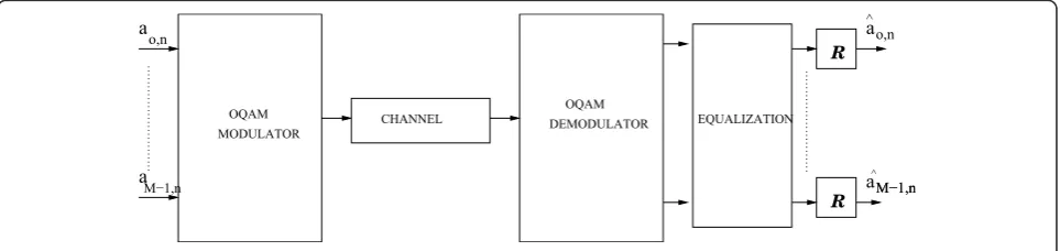
The block diagram in Figure 2 illustrates our OFDM/ OQAM transmission scheme. Note that compared to Figure 1, here a channel breaks the real orthogonality condition thus an equalization must be performed at the received side to restore this orthogonality.

Let us consider a channel h(t, τ ) that can also be represented by a complex-valued number _H(c)

m,n for

component h(t). For a locally invariant channel, we can define a neighborhood, denoted _m,n, around the (m0,n0) position, with

m,n=

(p, q), |p| ≤m, |q| ≤n|H(mc0)+p,n0+q≈H

(c)

m0,n0

and we also define ∗m,n=m,n−

(0, 0). Note also thatΔnandΔmare chosen according to the time and bandwidth coherence of the channel, respec-tively. Then, the demodulated signal [9-11] can be expressed as

y(mc)0,n0 =H

(c)

m0,n0(am0,n0+ja

(i)

m0,n0) +Jm0,n0+ηm0,n0, (5)

with ηm0,n0=η|gm0,n0 the noise component, a

(i)

m0,n0

the interference created by the close neighborhood given by

a(mi)0,n0=

(p,q)∈∗

m,n

am0+p,no+q g

m0,n0

m0+p,n0+q

and, finally, Jm0,n0 the interference created by the data

symbols outsideΩΔm,Δn. It can be shown that, even for small size neighborhoods, if the prototype function gis well localized in time and frequency, Jm0,n0 becomes

negligible when compared to the noise term ηm0,n0.

Indeed a good localization means that the ambiguity function ofg, which is directly related to the gm0,n0

m0+p,n0+q

terms, is concentrated around its origin in the time-fre-quency plane, i.e., only takes small values outside the ΩΔm,Δnregion. Thus the received signal can be approxi-mated by:

y(mc)0,n0 ≈H

(c)

m0,n0

am0,n0+ja

(i)

m0,n0

+ηm0,n0.

For the rest of the study, we consider (7) as the expression of the signal at the output of the OFDM/ OQAM demodulator. Now, if the channel is known at the receiver side, the estimate of the real transmit sym-bol can be easily obtained by a simple ZF or MMSE [12] equalization as:

ˆ

am0,n0 =

y(mc0),n0

H(mc)0,n0

=am0,n0+

ηm0,n0

H(mc)0,n0

. (8)

Concerning the channel, if the “pseudo-pilot”

bm0,n0 =am0,n0+ja

(i)

m0,n0 is known by the receiver, we can

compute an estimate of the channel by:

ˆ

H(mc)0,n0 =

y(mc0),n0

bm0,n0

=H(_mc)_0,n0+ηm0,n0

bm0,n0

. (9)

We talk about“pseudo-pilot” for bm0,n0 because a

(i)

m0,n0

is not transmitted but it is created at the receiver side. For clarity purpose, when in OFDM/OQAM we talk about real data transmitted at a given position (m, n), -I F F T P O L Y P H A S E P/S -S/P P O L Y P H A S E F F T P O S T -R{} R{} R{} M O D U D L A T I O N E -a0,n

a₁,n

aM−1,n P R E M O D L A T I O N U

Figure 1Transmultiplexer scheme for the OFDM/OQAM modulation.

^

ao,n

a^MM−−1,n1,n

OQAM MODULATOR OQAM DEMODULATOR CHANNEL EQUALIZATION o,n

M−1,n

a

a

R

R

we refer to it by am,n. However, when it is a real transmit pilot in a given position (m,n), we refer to it bypm,n.

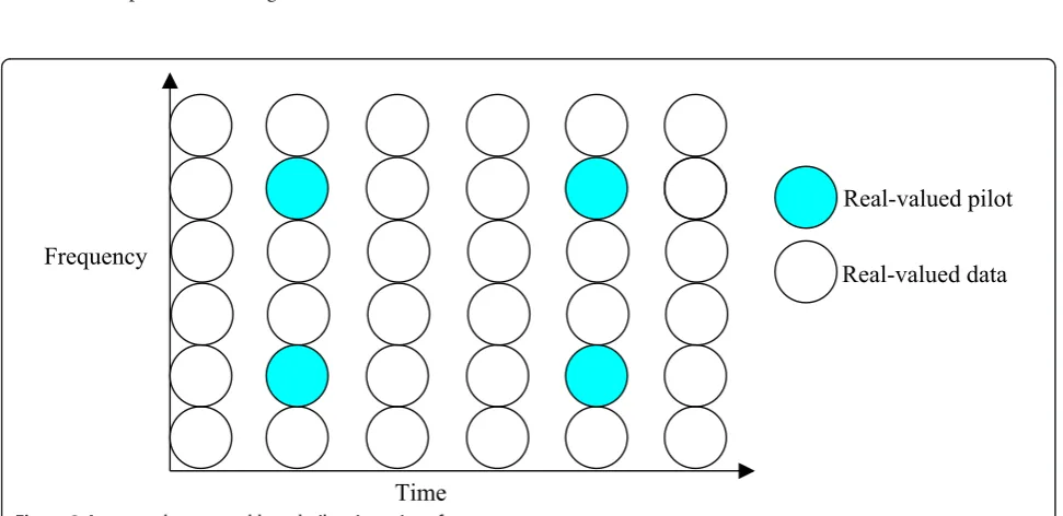
In a mobile environment, i.e., either the transmitter, the receiver or the transmission medium itself is mobile, the channel has to be continuously estimated. To do that pilots are inserted inside the transmitted frame at different time-frequency positions. We focus only on scattered-based CE, at a given position (m0, n0) a

real-valued pilot pm0,n0 is inserted and this pilot is

sur-rounded by real-valued data as illustrated in Figure 3. The receiver knows the values and the positions of the pilots and it wants to perform CE at these given posi-tions. Let us recall that for a real-valued pilot pm0,n0

located at the (m0, n0) position, the received signal at

this position is:

y(mc)0,n0 =H

(c)

m0,n0

pm0,n0+ja

(i)

m0,n0

+ηm0,n0. (10)

We want to estimate the channel coefficient _H(c)

m0,n0 at

this position. pm0,n0 is a real pilot that is known by the

receiver. _a(i)

m0,n0 depends on the data around this

posi-tion. These data are random so _a(i)

m0,n0 is random too.

The knowledge of a(mi)0,n0 at the receiver side is

manda-tory to perform any CE. However, a(mi)0,n0 is a linear

combination of data therefore it is unknown by the receiver. Methods should be derived in order to estimate the channel with low additional complexity and good performance. The methods proposed in this article will be studied by considering the simple OFDM/OQAM transmitter represented in Figure 4. The bits to be sent

are first channel encoded, e.g., using a convolutional code. Then the bits are mapped, e.g., using QPSK or 16-QAM modulation. From a complex symbol, cm,n the block denoted by C ® R provides two real data that correspond to the real and imaginary parts of the com-plex data. The real data, am,n, are modulated by an OFDM/OQAM modulator before transmission. Figure 4 does not include potential additional processing which is specific to each CE method. In CP-OFDM, if a pilot pm0,n0 is transmitted at a complex position (m0,n0) , the

received signal at this position is:

y(mc)0,n0 =H

(c)

m0,n0(pm0,n0) +ηm0,n0. (11)

Thus the channel is easily estimated. Having the same estimation process in OFDM/OQAM implies perform-ing some processperform-ing at the transmitter side. The pur-pose of the processing is to cancel _a(i)

m0,n0 at the receiver

side. Let us call these processing methods as imaginary interference cancelation.

3. Imaginary interference cancelation

3.1 Imaginary interference cancelation: principle

Imaginary interference cancelation purpose is to per-form some processing at the transmitter in order to can-cel _a(i)

m0,n0 at the receiver side. In order to simplify the

description of these methods, we assume that the ima-ginary interference can be approximated only using the data that are located just around the pilot position, i.e.,

a(mi)0,n0≈

(p,q)∈∗1,1

am0+p,no+q g

m0,n0

mo+p,n0+q. (12)

Frequency

Time

Real-valued pilot

Real-valued data

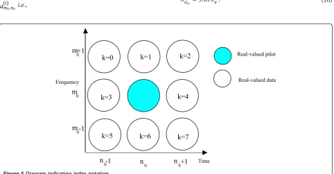
However, for the CE methods we propose the princi-ples can be extended to bigger neighborhood. To sim-plify the notations we use a single integer, k, to index the positions around the real pilot. Thus,ak is the real data around the real pilot at position kand gk is the value of gm0,n0

m0+p,n0+q at positionk. Figure 5 gives an

illus-tration of this notation. Then, we can write:

a(mi)0,n0 =

(p,q)∈∗

1,1

am0+p,no+qg

m0,n0

m0+p,n0+q=

7

k=0

akγk. (13)

Ideally, one would like to transmit eight random real data dk at the eight distinct positions, k= 0, 1 . . . 7, and to get a(mi)0,n0 = 0.That is naturally not possible in

general. 3.1.1 Method 1

The first idea is to transmit seven data at seven posi-tions i0, i1, i2, i3, i4, i5, i6 i.e., aik = dk with k Î [0,6]. At position i7 we transmit the value that will cancel

a(mi)0,n0 i.e.,

ai7 =−

6

k=0 aikγik

γi7

, (14)

then ai7 is not really a data. Indeed, this method

enables the estimation of the channel at (m0,n0)

posi-tion. However, the major problem with this method is the overall power used to estimate the channel. This power is actually the power transmitted in pm0,n0 plus

that used to transmit the signal corresponding to thei7 position. Based on (14), the power of ai7 can be high.

Indeed its average power is:

σ2

ai7 =σ

2

a

6

k=0

|γik| 2

|γi7|2

, (15)

with σ_a2 the power of the real dataam,n. As an exam-ple with IOTA prototype function [4], by takingi7 = 4,

we have:

σ2

ai7 = 5.07σ

2

a. (16)

Modulator OQAM

(x2)

C R

c_m,n a_m,n

Pilots Insertion Coding

Channel

Mapping b

Bits

Figure 4Conventional OQAM transmitter structure.

Time Frequency

Real-valued pilot

Real-valued data k=0

k=3

k=1 k=2

k=7

k=5 k=6

k=4 +1

m₀

m₀ m

0

-1

n 0 -1

n

0 n0+1

It is worth saying that using two real positions (the pilot position and the i7 position) for CE in OFDM/

OQAM is similar to use only one complex position in CP-OFDM.aThe drawback of using high power suggests that we should look for an other method.

3.1.2 Method 2

Let us look at another method to cancel _a(i)

m0,n0[10] gives

a particular rule to cancel _a(i)

m0,n0 only for an isotropic

prototype function like IOTA. This method has been extended in [1] which gives the general principle to get

a(mi)0,n0 ≈0 whatever the prototype filter being used. Let

us recall the main idea. Since dk is random, we could imagine to spread this piece of data over the eight posi-tions around the pilot, i.e., for each datadk,we associate a signature:

ck= [c0,k, c1,k, c2,k, c3,k, c4,k, c5,k,c6,k, c7,k]T.

Then, the symbolapbeing transmitted at positionpis the sum of all the contributions of the different data

given by: ap=

7

k=0cp,kdk∈[0; 7], i.e., by setting:

a

−= [a0,a1,a2,a3,a4,a5,a6,a7]T,d−= [d0,d1,d2,d3,d4,d5,d6,d7]T

C₋= (c0,c1,c2,c3,c4,c5,c6,c7),

we have, a₋=Cd. At the receiver side, to ensure the reconstruction of d₋from a₋, C₋ must be a non-singular matrix, thus d₋=C₋−1a₋. However it is important to choose C₋ orthonormal for two main reasons:

• C₋orthonormal implies that ||d₋|| = ||a₋||, because an orthonormal matrix preserves the norm.

•At the receiver side, the noise will be multiplied by C₋−1 which is also orthonormal. Using an orthonor-mal matrix prevents the noise power being increased while multiplying byC₋−1.

Let us set:γ₋= [γ0, γ1, γ2, γ3, γ4, γ5, γ6, γ7]T, where

γ

−= 08(08 is the null element for addition in R 8

). We have:

a(mi)0,n0=

7

p=0 apγp=

7 p=0 γp 7 k=0 cp,kdk=

7 k=0 ₇ k=0

γpcp,k

dk=

7

k=0

γ₋T_c

k

dk (17)

To havea(mi)0,n0 = 0, whatever thedkvalues, a necessary

and sufficient condition is to have: γ₋Tck= 0 for

allk∈[0; 7], i.e., (c0, c1, c2, c3, c4, c5, c6, c7, γ₋) must be orthogonal. This is not possible because nine vectors

cannot form an orthogonal basis in a vector space of dimension eight. One constraint must be free, that is, either we set one piece of data to be null for example d7= 0, or we have a linear relationship between data, i. e., one piece of data is a linear combination of others. Let us set d7= 0, that is:

a(mi)0,n0=

6

k=0

γ₋T

ck

dk (18)

The condition is now that:

⎛ ⎜ ⎜

⎝c0, c1, c2, c3, c4, c5, c6,

γ₋ γ₋ ⎞ ⎟ ⎟

⎠ forms an orthonormal

basis of R8, which is now possible. For a given γ−, it is possible to find many C₋ matrices either by using Schmidt orthogonalization [13] for generating orthonor-mal basis of R8 _{or another method that we suggest in} [1] for complexity reduction. To summarize, at position (m0,n0), where the channel must be estimated, we:

(1) Introduce a real pilot at that position;

(2) Replace the data around the pilot position by other data resulting from the product of C₋ with the initial data;

(3) Modulate and transmit the overall data.

At the receiver side, after demodulation, at any posi-tion (m0,n0) the signal can be written as given by (7). At

the pilot position, we have:

a(mi)0,n0 ≈

(p,q)∈∗1,1

am0+p,no+qg

m0,n0

m0+p,n0+q= 0 (19)

i.e.,

y(mc0),n0 ≈H

(c)

m0,n0(pm0,n0) +ηm0,n0 (20)

the estimate of the channel at this position is obtained by:

ˆ

Hm(c)0,n0 =

y(mc0),n0

pm0,n0

≈H(_mc_0,)_n0+ηm0,n0

pm0,n0

(21)

Using interpolation techniques [14], an estimate of the channel over all the positions (m, n) can be derived. Then, using (8), we obtain an estimate of the real trans-mitted data. Around the pilot position, the transtrans-mitted data were obtained after multiplying the initial data by C₋. To have an estimate of the initial data, we must

However, it implies one matrix computation at each pilot position this at the transmitter and receiver. Thus, it increases the complexity.

3.2 Performance of the imaginary interference cancelation method

Let us look at the performance of the interference can-celation method using the matrix cancan-celation process previously presented. We use the approximation in (12). Our simulations have been carried out with the follow-ing channel profile and parameters:

•Sampling frequencyfs=9.14 MHz;

•Number of paths: 6;

•Power profile (in dB) :−6.0, 0.0,−7.0, −22.0,−16.0,

−20.0;

• Delay profile (μs):-3, 0, 2, 4, 7, 11. We denote by

Δthe maximum delay spread of the channel (Δ=11μ s);

•Guard interval composed of 130 samples(14.22μs);

•QPSK and 16-QAM modulations;

• FFT size M = 1024; Let denote byTu the useful

CP-OFDM symbol duration:Tu =

M fs

• Convolutional channel coding (K= 7with genera-tors g1 = (133)o,g2 = (171)o, in octal form and code

rate= 1 2);

•Frame structure of DVB-T2 standard [3];

•The velocity is 5 km/h;

•The zero forcing equalization technique is used;

•Prototype filter used: IOTA4 and TFL1;

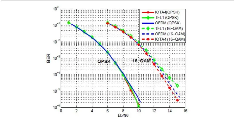
For OFDM/OQAM, we use the matrix transformation presented to cancel the interference and estimate the channel. The performance is evaluated by the bit error rate (BER) as a function of the Eb/N0 ratio. Figure 6

shows that for the QPSK modulation, IOTA4 and TLF1 have approximately the same performance and outper-form CP-OFDM by less than 0.3dB. This gain corre-sponds to the no use of GI. For the 16-QAM modulation, IOTA4 is slightly better than CP-OFDM with about 0.2 dB gain thanks to the no use of GI, whereas CP-OFDM is 0.2dB better than TFL1 at BER = 10−4. The main reason for such a difference is that, we have made the approximation in (12) which is equiva-lent to consider thatΔm=Δn= 1.

By considering this approximation, we have: E|Jm0,n0|

2_≈0.05σ2

a for TFL1. Thus when the Eb/N0

value comes close to 13dB, Jm0,n0 in (5) is not negligible

compared to the noise term. Consequently, the perfor-mance of TFL1 deteriorates for Eb/N0 around 13dB.

Whereas for IOTA4, E|Jm0,n0|

2_≈0.014σ2

a, thus the

degradation of performances is likely to appear around 18.5 dB. It is worth saying that the exact value of Δm andΔn is not 1. Indeed, if we consider that the

coher-ence bandwidth is about Bc= 1

then,Δmis about:

m=TuBc 2 =

M

2fe ≈ 5.

Thus, by considering the approximation of _a(i)

m0,n0 for

Δm= 5 the result for TFL1 should be better.

In this section, the purpose has been to cancel the imaginary interference at pilots positions in order to achieve a simple equalization. How about using this interference term at the receiver side to improve the CE?

4. Iterative CE method

4.1 The iterative CE method: principle

In this section, we present a new CE method [2] which involves the estimation of _a(i)

m0,n0 at the pilot position and

at the receiver side. From (10), the CE is performed by:

ˆ

Hm(c0),n0= y(mc)0,n0 pm0,n0+jˆa

(i)

m0,n0

=H(mc)0,n0 pm0,n0+ja

(i)

m0,n0 pm0,n0+jaˆ

(i)

m0,n0

+ ηm0,n0 pm0,n0+jaˆ

(i)

m0,n0

(22)

with a_ˆ(mi)0,n0 an estimate of a

(i)

m0,n0. Let us recall that

a(mi)0,n0 =

(p,q)∈∗m,n

am0+p,no+qg

m0,n0

m0+p,n0+q (23)

Let us recall that we consider the OFDM/OQAM transmitter represented in Figure 4. At the receiver side, we first present the ideal structure where the receiver has the perfect knowledge of the “pseudo-pilot” bm0,n0 =pm0,n0+ja

(i)

m0,n0 as described in Figure 7. The

receiver structure performs the following operations: (1) OFDM/OQAM demodulation;

(2) A CE is performed at the pilot position using (22), with a_ˆ(mi)0,n0 =a

(i)

m0,n0. Then, using an interpolation

techni-que, an estimate of the whole channel is derived in every time-frequency position;

(3). Then the equalization of the demodulated signal can be performed. By taking the real part (block R) of the equalized signal, we obtain an estimate of the real data;

(4). The block R®C in Figure 7, reconstructs the complex symbol from the two real data, then the demapping operation generates the soft bits;

• The decoded bits which are the estimates of the transmitted bits.

• The soft or hard (soft/hard) coded bits which are the metric values that are generally used for the iterative process [15].

The process from 3 to 5 designated as bits recovering, permits an analogy between Figures 7 and 8 and it is used to introduce the iterative CE method. Again, the processes 4 and 5 are referred to be the real data to bits

process and are used to make the analogy between Fig-ures. 9 and 7. However, the imaginary part a(mi)0,n0 of the

“pseudo-pilot” bm0,n0 is unknown by the receiver. We

suggest to estimate a(mi)0,n0 in an iterative manner. We

start with a_ˆ(mi)0,n0 = 0 at the first iteration. This

corre-sponds to the mean value. Then from (22) a first CE is obtained. Using it and applying the bits recovering block (cf. Figure 7) soft/hard coded bits are obtained. From these soft/hard coded bits, we generate an estimate

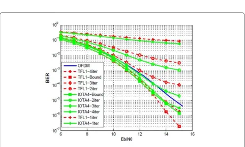
Figure 6Performance of Imaginary Interference Cancelation method with IOTA4, TFL1 and CP-OFDM ones in scattering environment (velocity 5 km h−1).

Demodulator OQAM

(1/2)

R

c_m,n ^ a_m,n

^ Equalization

Channel Estimation

pseudo-pilots

Decoding Soft/Hard coded bits Demapping Channel

Perfect

Decoded bits Bits Recovering

of the data am0+p,n0+q around the pilot position(m0,n0).

n indicates the iteration number. These data are then used to compute another estimate of a(mi)0,n0(23) by:

ˆ

a(mi)0,n0 =

(p,q)∈∗m,n

ˆ

a(mn0)+p,n0+qg

m0,n0

m0+p,n0+q. ₍₂₄₎

Then, the process should be reiterated and a new CE can be performed using (22) with this new “ pseudo-pilot”estimation value. Then, the bits recovering block gives new decoded bits and soft/hard coded bits. The process can be repeated n times.

4.2 Advantages of the iterative CE method

There are two main advantages with the iterative CE method.

First advantage: The first advantage is that, assuming a perfect estimation, then the power of the “pseudo-pilot” bm0,n0, is the power of the transmitted pilot pm0,n0 plus

the power of a(mi)0,n0i.e.,

E|bm0,n0|

2_=E|p

m0,n0|

2_+E|a(i)

m0,n0|

2 ₍₂₅₎

The power of the transmitted pilot denoted byP2, is taken similar in OFDM/OQAM and in CP-OFDM, i.e., E|pm0,n0|

2_=P2_≥σ2

c = 2σa2, with σa2 the power of the

real dataam,nand σc2the power of the complex data as

in CP-OFDM. Let us recall that, the power of the trans-mitted pilot is greater than σc2 when boosting is used.

In [16], we show that E|a(mi)0,n0|

2_≈σ2

a. Therefore,

in OFDM/OQAM the power of the“pseudo-pilot” is:

E|bm0,n0|

2_≈P2_+σ2

a (26)

showing that its power is greater than in CP-OFDM. This virtual boosting in OFDM/OQAM is due to the interference terma(mi)0,n0, which is added in a constructive

way to the transmit pilot. This implies that the CE should be better in OFDM/OQAM than in CP-OFDM, leading to potentially better performance for OFDM/OQAM. DemodulatorOQAM Bits Recovering

Channel

Estimation Estimation Estimation

Pseudo-Pilot

Decoded bits

Soft/Hard coded bits

Figure 8Iterative OFDM/OQAM receiver block diagram.

DemodulatorOQAM Equalization

R

Channel Estimation

Pseudo-Pilot Estimation

Real data to bits process

Decoded bits

Soft/Hard coded bits

Second advantage: The second advantage with this OFDM/OQAM CE is that the transmit pilot in OFDM/ OQAM is a “real-based” symbol and not a “ complex-based” one as in CP-OFDM. Therefore, the percentage of the overhead pilots with this CE method should be half the one required for CP-OFDM. As an example, in DVB-T2 standard [3], we have about 8.33% of pilots into the CP-OFDM frame. For OFDM/OQAM, this CE method leads to an overhead of 4.16%. This leads to a gain in spectral efficiency, because we can transmit a real data information symbol each time we transmit a real pilot. However, in order to have a fair comparison in terms of transmit power between CP-OFDM and OFDM/OQAM, the powerP2 of the pilot has to be split in OFDM/OQAM between the transmitted pilot and the extra data. So in OFDM/OQAM, if we add an addi-tional real data each time we transmit a pilot, the pilot power should be P2−σ_a2 and the additional real data power being σa2. Thus the power of bm0,n0 becomes:

E|bm0,n0|

2_≈P2_{; Leading to no gain in terms of CE}

when compared to CP-OFDM.

We have a tradeoff to make between either adding no additional data and gain in CE in OFDM/OQAM or having higher spectral efficiency without gain in CE. We can also choose to add additional data for some pilots and no extra data for others. It is worth noticing that if we choose not to add this extra data, then a null value (0) is transmitted each time a pilot is sent. Therefore this knowledge could be, for example, used by the recei-ver to improve the synchronization process or used to have an estimate of the noise power density. Figure 10 is a “pseudo-pilot” representation at the receiver side. The first iteration, that corresponds to the approxima-tion of the“pseudo-pilot”by the transmit pilot, is a kind of blind estimation (it is the mean“pseudo-pilot”value). Therefore, we hope to converge as the number of itera-tions increases. However, iteration implies additional memories and processing-delay. To reduce the delay, we suggest to implement the receiver structure of the

Figure 9 where iterations are done without using the channel decoding block inside the iterative process, i.e., the iterations are done on“real data basis”. After taking the real part of the equalized-signal, we have an estimate

ˆ

am,n of the real transmitted data. These estimates are

used to perform another “pseudo-pilot” estimation thanks to (24), leading to obtain another CE and another real data detection. The process can be repeated ntimes. At the last iteration, the real data estimates are used to reconstruct the complex symbol (blockR®C), then the demapping process generates soft bits that are used by the channel decoding to recover the transmitted bits.

4.3 Simulations

We have performed simulations and made comparisons, using the system and channel parameters defined in Section 3. We have evaluated the performance of both receivers, i.e., either by implementing or not the decod-ing into the iteration process (IP). IOTA4-Bound (Resp. TFL1-Bound) corresponds to the case where we assume that the term a(mi)0,n0 is perfectly known by the receiver

at the pilot position. IOTA4-niter (Resp. TFL1-niter) corresponds to the case where we implement the pre-sented algorithm withniterations.n= 1 corresponds to a non-iterative case. When considering channel decod-ing inside the IP, IP, as shown in Figure 8, we have used a hard decoding procedure.

4.3.1 Performances with decoding inside the IP process Let us look at the performances when channel decoding is used inside the IP, as depicted in Figures 11 and 12 for QPSK and 16-QAM modulation, respectively. For this analysis, we consider a BER interval between 10−4 and 10 −5. In QPSK modulation, we note that IOTA4-Bound and TFL1-IOTA4-Bound are close and outperform CP-OFDM by about 1 dB. As the number of iterations increases, we get closer to the limit bound. Three itera-tions allow to achieve the bound. IOTA4-1iter and TFL1-1iter performance are very bad compared to

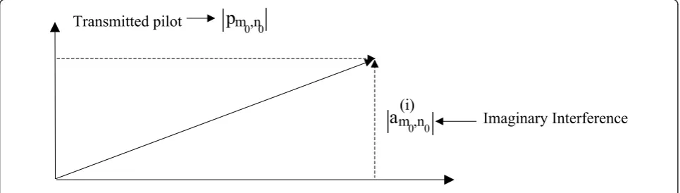
CP-m ,n

p

0

m ,n

a

|

|

|

(i)

|

Imaginary Interference

Transmitted pilot

100 200 300 400 500 600

Figure 11BER results for one-half coded QPSK at different iteration stages, using the decoding inside the IP.

100 200 300 400 500 600

OFDM, since we consider a_ˆ(mi)0,n0 = 0. IOTA4-2iter and

TFL1-2iter perform approximately the same with 0.3 dB gain comparing to CP-OFDM. With 16-QAM modula-tion in Figure 12, TFL1-Bound is slightly better than IOTA4-Bound for Eb/N0 greater than 13 dB. This

method is not limited by the approximation (12) as it was the case for imaginary interference cancelation. It is illustrated by the fact that TFL1-Bound does not dete-riorate for Eb/N0 greater than 13 dB. However the

shorter is the prototype length the smaller could be the number of terms involved when computing _a(i)

m0,n0 in

(6). The am0+p,n0+q data in (6) are those which have

approximately the same channel coefficient as am0,n0.

Having more terms am0+p,n0+q implies more errors when

considering their channel coefficients to be equal to am0,n0 channel coefficient. This can justify why

TFL1-Bound is slightly better than IOTA4-TFL1-Bound since TFL1 is shorter than IOTA4. IOTA4-Bound outperforms CP-OFDM by about 1 dB. With four iterations, we are very close to the limit bound for both prototypes. IOTA4-3iter (Resp. IOTA4-2iter and Resp. IOTA4-1iter) per-forms better than TFL1-3iter (Resp. TFL1-2iter and Resp. TFL1-1iter) with a gain which can be higher than 2 dB. CP-OFDM outperforms IOTA4-1iter by more than 3 dB, whereas IOTA4-2iter is closer to the CP-OFDM. IOTA4-1iter and TFL1-1iter’s performance are very bad compared to CP-OFDM, since we consider

ˆ

a(_mi)_0,n0= 0. Thus, three iterations allow us to be close to

CP-OFDM performance and four iterations are neces-sary to outperform CP-OFDM by about 1 dB. Thus, using decoding in the IP process leads to better perfor-mances when comparing with CP-OFDM.

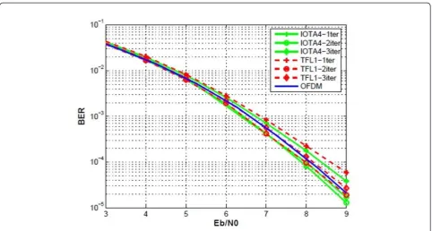
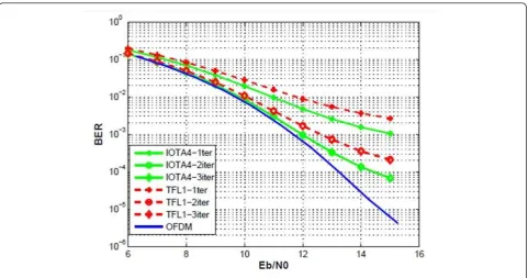
4.3.2 Performances without decoding inside the IP process Let us consider the performances obtained without con-sidering the decoding inside the IP process as shown in Figure 9. Figures 13 and 14 give the performance for QPSK and 16-QAM modulation, respectively. From these figures, we find thatn= 2 iterations are sufficient for con-vergence purpose. Indeed, forn= 3 the performance is slightly less than withn= 2. Thus more iterations will bring nothing. In QPSK with two iterations we do better than CP-OFDM with about 0.2 dB gain. Whereas in 16-QAM for BER less than 10−4, we lose more than 1.5 dB. Thus, when the channel decoding is not used inside the IP, performance are either of same order or worse than those of CP-OFDM. Including the decoding into the IP (cf. Figure 8) gives better performance but processing delay is higher than the scheme without the decoding inside the IP (cf. Figure 9). Consequently, one can choose to combine the both types of iteration in order to have the good tradeoff between performance and processing delay. Let us say the two first iterations can be done without the decoding inside the IP, while the following iterations are done with decoding block inside the IP.

5. Conclusion

In this article, we have shown that the CE in OFDM/ OQAM cannot be performed in the same way as in

OFDM modulation. The imaginary interference cancela-tion method provides a mean to estimate in a similar way the channel as in CP-OFDM and its performances are closer to CP-OFDM ones. The article has presented an iterative CE method, which uses the imaginary inter-ference at the receiver side to improve the CE. This is done by an iterative estimation of the imaginary inter-ference using either the decoding block inside or not the IP. Comparisons with CP-OFDM show indeed that when the decoding block is used inside the IP the per-formances of OFDM/OQAM modulation outperform CP-OFDM ones as long as both modulations have the same transmitted pilot power. Iterative CE method sug-gests that the imaginary interference can be used posi-tively, how about trying to use it in order to improve the data estimation process?

Endnote a

The two real positions can be viewed as the real and imaginary parts of a complex position.

Competing interests

The author declares that he has no competing interests.

Received: 23 February 2011 Accepted: 22 February 2012 Published: 22 February 2012

References

1. C LTlT, P Siohan, R Legouable, Channel estimation with scattered pilots in OFDM/OQAM, inSPAWC 2008, Recife, Brazil, pp. 286_–290 (June 2008)

2. C LTlT, P Siohan, R Legouable, Iterative scattered pilot channel estimation in OFDM/OQAM, SPAWC 2009, Perugia, Italy, pp. 176–180 (June 2009) 3. ETSI, Frame structure channel coding and modulation for a second generation digital terrestrial television broadcasting system (DVB-T2). European standard DVB document A122 (June 2008)

4. B Le Floch, M Alard, C Berrou, Coded orthogonal frequency division multiplex, inProceedings of the IEEE, vol. 83. Cesson Sevigne, France, pp. 982–996 (June 1995). doi:10.1109/5.387096

5. B Hirosaki, An orthogonally multiplexed QAM system using the discrete Fourier transform. IEEE Trans Commun.29(7), 982–989 (1981). doi:10.1109/ TCOM.1981.1095093

6. H B_œlcskei, Orthogonal frequency division multiplexing based on offset QAM, Advances in Gabor Analysis, BirkhSuser, Boston (2003)

7. P Siohan, C Siclet, N Lacaille, Analysis and design of OFDM/OQAM systems based on filterbank theory. IEEE Trans Signal Process.50(5), 1170–1183 (2002). doi:10.1109/78.995073

8. P Siohan, D Pinchon, C Siclet, Design techniques for orthogonal modulated filterbanks based on a compact representation. IEEE Trans Signal Process.

52(6), 1682–1692 (2004). doi:10.1109/TSP.2004.827193

9. D Lacroix-Penther, J-P Javaudin, A new channel estimation method for OFDM/OQAM, inProc. of the 7th International OFDM workshop, Hamburg, Germany (10–11 Sept 2002)

10. J-P Javaudin, D Lacroix, A Rouxel, Pilot-aided channel estimation for OFDM/ OQAM, inVTC’03 Spring, vol. 3. Cesson Sevigne, France, pp. 1581–1585 (April 2003)

11. C Lele, P Siohan, R Legouable, M Bellanger, CDMA transmission with complex OFDM/OQAM. Eurasip J Wirel Commun Netw.2008, 12 (2008) 12. J Bibby, H Toutenburg, Prediction and Improved Estimation in Linear

Models, (Wiley, New York, 1977)

13. H Cohen, A Course in Computational Algebraic Number Theory, (Springer, New York, 1993)

14. S Kaiser, P Hoeher, P Robertson, Two-dimensional pilot-symbol-aided channel estimation by Wiener filtering, inICASSP 97, Munich, pp. 1845–1848 (21_–24 April 1997)

15. C Laot, A Glavieux, J Labat, Turbo equalization over a frequency selective channel. International Symposium on Turbo Codes and Related Topics (1997)

16. C Lele, J-P Javaudin, R Legouable, A Skrzypczak, P Siohan, Channel estimation methods for preamble-based OFDM/OQAM modulations, European Wireless, Paris, France (1–4 Apr 2007)

doi:10.1186/1687-6180-2012-42

Cite this article as:Lélé:Iterative scattered-based channel estimation method for OFDM/OQAM.EURASIP Journal on Advances in Signal Processing20122012:42.

Submit your manuscript to a

journal and benefi t from:

7Convenient online submission

7Rigorous peer review

7Immediate publication on acceptance

7Open access: articles freely available online

7High visibility within the fi eld

7Retaining the copyright to your article