Adaptive Inverse Hyperbolic Tangent Algorithm for Dynamic Contrast Adjustment in Displaying Scenes

(1)

Volume 2010, Article ID 485151,20pages doi:10.1155/2010/485151

Research Article

Adaptive Inverse Hyperbolic Tangent Algorithm for Dynamic

Contrast Adjustment in Displaying Scenes

Cheng-Yi Yu,

1, 2

_{Yen-Chieh Ouyang,}

1

_{Chuin-Mu Wang,}

2

_{and Chein-I Chang}

3

1_{Department of Electrical Engineering, National Chung Hsing University, Taichung 402, Taiwan}

2_{Department of Computer Science and Information Engineering, National Chin Yi University of Technology, Taichung 411, Taiwan}

3_{Remote Sensing Signal and Image Processing Laboratory, Department of Computer Science and Electrical Engineering,}

University of Maryland, Baltimore County, Baltimore, MD 21250, USA

Correspondence should be addressed to Yen-Chieh Ouyang,[email protected]

Received 16 November 2009; Accepted 11 February 2010

Academic Editor: Yingzi Du

Copyright © 2010 Cheng-Yi Yu et al. This is an open access article distributed under the Creative Commons Attribution License, which permits unrestricted use, distribution, and reproduction in any medium, provided the original work is properly cited.

Contrast has a great influence on the quality of an image in human visual perception. A poorly illuminated environment can significantly affect the contrast ratio, producing an unexpected image. This paper proposes an Adaptive Inverse Hyperbolic Tangent (AIHT) algorithm to improve the display quality and contrast of a scene. Because digital cameras must maintain the shadow in a middle range of luminance that includes a main object such as a face, a gamma function is generally used for this purpose. However, this function has a severe weakness in that it decreases highlight contrast. To mitigate this problem, contrast enhancement algorithms have been designed to adjust contrast to tune human visual perception. The proposed AIHT determines the contrast levels of an original image as well as parameter space for different contrast types so that not only the original histogram shape features can be preserved, but also the contrast can be enhanced effectively. Experimental results show that the proposed algorithm is capable of enhancing the global contrast of the original image adaptively while extruding the details of objects simultaneously.

1. Introduction

Digital cameras, which have gradually replaced conventional cameras, store photographs in a digital format. However, this

is not the only way in which digital cameras diﬀer from

conventional cameras. In conventional machinery cameras, the diaphragm and focal distance are adjusted by the photographer to obtain better scenes. Digital cameras, on the contrary, capture scenes using a sensor which might record a tremendous amount of energy from one material in a certain wavelength, while recording another material at much less energy in the same wavelength. Besides, the photographer cannot adjust the diaphragm or focal distance.

In real-world situations, light intensities have a large range. At the low end, the average intensity of starlight is

approximately 10−3_cd/cm2 _{and a sunny day can produce a}

high light intensity of 105_cd/cm2_{or more. However, the}

visi-ble range perceived by the human eye is only 1 to 104_cd/cm2_.

As a result, we lose almost all the details appearing in the darkest and brightest ranges of the visible spectrum. Today,

most digital video cameras have the capability of capturing high dynamic range (HDR) images with a luminance level of 200% to 600%. Nevertheless, most display devices are only capable of a low dynamic range (LDR), with a luminance

level of about 110% [1].

Visual adaptation in humans provides us with the ability to see in a wide range of conditions, from the darkness of night to the brightness of the midday sun. Adaptation means that the signals from our photoreceptors are processed to amplify weak signals and weaken strong signals, thereby preventing saturation. The previous physiological research shows that ganglion cells, the output cells of the retina, adapt at lower light levels than cones horizontal cells, one

of the downstream targets of the cones [2]. This provides

evidence for adaptation in the retinal circuitry and in the cone photoreceptors, known as receptor adaptation. As light levels increase, the main site of adaptation switches from the retinal circuitry to the cone photoreceptors.

(2)

6 5 4 3 2 1 0 −1 −2 −3 −4 −5 −6

logL(d/m2₎

0 0.2 0.4 0.6 0.8 1

R/

Rmax Rod Cone

Star light Moon light Oﬃce light Day light

Figure1: Human visual system mapping curve.

680 640 600 560 520 480 440 400

Wavelength (nm) 0

0.02 0.04 0.06 0.08 0.1 0.12 0.14 0.16 0.18 0.2

F

ra

ct

ion

of

lig

h

t

absor

b

ed

b

y

ea

ch

ty

p

e

o

f

cone

B

R

G

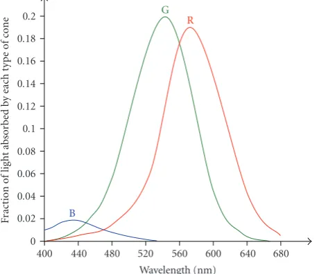
Figure2: Sensitivity of the cones.

contain pigments that absorb visible light to give us the sense of vision. The rods, which are numerous, are spread all over the retina and respond only to light and dark. They are very sensitive and can respond to a single photon of light. There

are about 110,000,000 to 125,000,000 rods in the eye [3].

The other type of cell is the cones located in one small area of the retina (the fovea). Their number is about 6,400,000. These cells are sensitive to colors but require more intense light in the order of hundreds of photons. Incidentally, the

cones are very sensitive to red, green, and blue (Figures1and

2) [4,5], which is the reason why monitors use these colors

as primaries. There are three types of cones: A, B and, C cones. The A cones are sensitive to red light, and the B cones are sensitive to green light (slightly more than the A cones). The C cones are sensitive to blue light, but their sensitivity is about 1/30 that of the A or B cones.

The human eye features a much higher resolution than

cameras but its eﬀective resolution is even higher when we

consider that the eye can move and refocus itself about three to four times a second. This means that in a single second the eye can sense and send to the brain about half a billion pixels.

The eye is a complex biological device. A camera is often compared to an eye because both focus the light from external objects in the visual field into a light-sensitive medium. In the case of the camera, this medium is film or an electronic sensor as opposed to the eye which is an array of visual receptors. According to the laws of optics, this simple geometrical similarity means that both eyes and a CCD camera function as transducers.

Light entering the eye is refracted as it passes through the cornea. It then passes through the pupil (controlled by the iris) and is further refracted by the lens. The cornea and lens act together as a compound lens to project an inverted image onto the retina.

A common problem in digital cameras is that the range of reflectance values collected by a sensor may not match the capabilities of the digital format or color display monitor. So, image enhancement techniques are generally required to make an image easier to analyze and interpret. The range of brightness values within an image is referred to as contrast. The contrast enhancement is a process that makes the image features stand out more clearly by optimizing the colors available on the display or an output device. A contrast enhancement algorithm allows users to custom design to improve image quality, representation, and interpretation.

Many factors contribute to image quality including brightness, contrast, noise, color reproduction, detail repro-duction, visual acuity simulation, glare simulation, and artifacts. In so doing various digital images processing techniques have been developed. Among them is the con-trast enhancement which plays the most important role

in increasing the visual quality of an image [6, 7]. For

this reason, the contrast enhancement has been the major approach to improve image quality.

According to image contrast an images is generally categorized into one of five groups: dark image, bright image, back-lighted image, low-contrast image, and high-contrast image. A dark image has particular low gray levels in intensity, while a bright image has very high gray levels in intensity. The gray levels of a back-lighted image are usually distributed at the two ends of dark and bright regions. On the other hand, the gray levels of a low-contrast image are generally centralized on the middle region, while the gray levels of a high-contrast image are scattered across the whole

spectrum (Figure 3) [8].

Five categories of commonly used gray level transfer

functions shown inFigure 4are generally used to perform

contrast enhancement so as to achieve diﬀerent types of

contrast [8]. For example, for dark images with mean<0.5,

the function inFigure 4(a)is used; whereas the function in

Figure 4(b)is used for a bright image with mean>0.5 for the

same purpose. For images whose gray levels are centralized in the middle region with mean near at 0.5, the function

in Figure 4(c) is used. For images whose gray levels are

distributed at the two end of dark and bright region, the

function inFigure 4(d)is used. For the images whose gray

levels are uniformly scattered across the whole spectrum, the

function inFigure 4(e)is used.

(3)

r

Dark image

p(r)

(a)

r

Bright image

p(r)

(b)

r

Back-lighted image

p(r)

(c)

r

Low-contrast image

p(r)

(d)

r

High-contrast image

p(r)

(e)

Figure3: Five kinds of contrast types.

that is suitable for interactive applications. It can automat-ically produce contrast enhanced images with good quality while using a spatially uniform mapping function that is based on a simple brightness perception model to achieve

better eﬃciency. In addition, the AIHT also provides users

with a tool of tuning the on-the-fly image appearance in terms of brightness and contrast and thus is suitable for interactive applications. The AIHT-processed images can be reproduced within the capabilities of the display medium to have better detailed and faithful representations of original scenes.

The remainder of this paper is organized as follows.

Section 2reviews the previous work done in the literature.

Section 3 develops the AIHT contrast enhancement

algo-rithm along with its parameters and usage. Section 4

con-ducts experiments including simulations. Finally, Section 5

provides future directions of further research.

2. Contrast Enhancement for an Image

Each pixel in a gray-scaled image has brightness ranging from 0 to 255 with the values of 0 and 255 representing black and white, respectively. A histogram shows the number of pixels with the various levels of brightness. The “0” value on the left of a histogram shows the number of pixels that are black, while the “255” value on the right indicates the number of pixels being white. Normalizing the histogram by the total number of pixels in the image produces a probability distribution of brightness levels.

Since a digital image is encoded byLbits, the gray level

of brightness varies from 0 to 2L−1_{. Assume that}_r

kis thekth

gray level. Its probability is defined by

P(rk)=nk

N, (1)

wherenk is the number of pixels specified by rk, and N is

the total number of pixels in the image. If the histogram of an image has a narrow dynamic range, it will be a

low-contrast image. In this case, diﬀerent objects in the image

will have their brightness in nearly the same gray level range

which may cause diﬃculty in object identification, object

classification, and image processing. Under such a circum-stance the contrast enhancement is generally performed to expand gray level range to mitigate the problem. One popular technique to accomplish this task is histogram equalization

in (Gonzalez and Woods [9]).

There are two categories of contrast enhancement tech-niques: global methods and local methods. The advantages

of using a global method are its high eﬃciency and

(4)

1 0.9 0.8 0.7 0.6 0.5 0.4 0.3 0.2 0.1 0

Input level 0

0.1 0.2 0.3 0.4 0.5 0.6 0.7 0.8 0.9 1

Output

le

ve

l

Bias=0.37, gain=0.35

(a)

1 0.9 0.8 0.7 0.6 0.5 0.4 0.3 0.2 0.1 0

Input level 0

0.1 0.2 0.3 0.4 0.5 0.6 0.7 0.8 0.9 1

Output

le

ve

l

Bias=0.37, gain=3

(b)

1 0.9 0.8 0.7 0.6 0.5 0.4 0.3 0.2 0.1 0

Input level 0

0.1 0.2 0.3 0.4 0.5 0.6 0.7 0.8 0.9 1

Output

le

ve

l

Bias=0.97, gain=1

(c)

1 0.9 0.8 0.7 0.6 0.5 0.4 0.3 0.2 0.1 0

Input level 0

0.1 0.2 0.3 0.4 0.5 0.6 0.7 0.8 0.9 1

Output

le

ve

l

Bias=0.97, gain=1

(d)

1 0.9 0.8 0.7 0.6 0.5 0.4 0.3 0.2 0.1 0

Input level 0

0.1 0.2 0.3 0.4 0.5 0.6 0.7 0.8 0.9 1

Output

le

ve

l

Bias=0.37, gain=1

(e)

Figure4: Five categories of commonly used gray level transform functions: (a) dark image, (b) bright image, (c) back-lighted image, (d)

(5)

1 0.9 0.8 0.7 0.6 0.5 0.4 0.3 0.2 0.1 0

Input luminance

β=2

β=3

β=5

β=10

β=20

0 0.1 0.2 0.3 0.4 0.5 0.6 0.7 0.8 0.9 1

Output

lu

minanc

e

Logarithm curve

Figure5: Logarithm curve for diﬀerentβ’s value.

2.1. Linear Contrast Enhancement. Linear contrast enhance-ment is also referred to as contrast stretching. It linearly expands the original digital luminance values of an image to a new distribution. Expanding the original input values of the image makes it possible to use the entire sensitivity range of the display device. Linear contrast enhancement also highlights subtle variations within the data. This type of enhancement is best suitable to remotely sensed images with Gaussian or near-Gaussian histograms. There are three methods of linear contrast enhancement.

2.1.1. Minimum-Maximum Linear Contrast Stretch. The minimum-maximum linear contrast stretch assigns the original minimum value to the new minimum value and the original maximum value to the new maximum value where the original intermediate values are scaled proportionately between the new minimum and maximum values. Many digital image processing systems can automatically expand these minimum and maximum values to optimize the full range of available brightness values.

2.1.2. Percentage Linear Contrast Stretch. The percentage linear contrast stretch technique is similar to the minimum-maximum linear contrast stretch except that the minimum and maximum values are found in a way that the values between them cover a given percentage of pixels from the mean of the histogram. A standard deviation from the mean is often used to push the tails of the histogram beyond the original minimum and maximum values.

1 0.9 0.8 0.7 0.6 0.5 0.4 0.3 0.2 0.1 0

Input level 0.3

0.4 0.5 0.65 0.8 1

1.25 1.6 2.1 2.8 3.8 0

0.1 0.2 0.3 0.4 0.5 0.6 0.7 0.8 0.9 1

Output

le

ve

l

Adaptive power function curve

Figure6: Gamma function curve for diﬀerentγ’s value.

2.1.3. Piecewise Linear Contrast Stretch. When the distribu-tion of an image histogram is a bi- or tri-modal, it is possible to stretch certain values of the histogram to increase contrast enhancement in selected areas. The piecewise linear contrast enhancement involves the identification of a number of linear enhancement steps that can expand the brightness ranges in multiple modes of the histogram. Compared to a normal linear contrast stretch which stretches the minimum and maximum values to the values of lowest and highest gray levels linearly at a constant level of intensity, the piecewise linear contrast stretch defines several breakpoints that increase or decrease the contrast of the image for a given range of values. A low-slop of an image histogram produces a lower contrast for the same range of values. On the other hand, a high-slop of an image histogram produces a higher contrast for the same range of values. So, the higher the slope,

the narrower the range of values mapped from thex-axis.

This approach creates a wider spread output for the same original values, thus increasing the contrast for that range of values. A piecewise stretch method performs a series of small min-max stretches within a single histogram and is very useful in contrast enhancement. This benefit is traded

oﬀfor that image analysts must be very familiar with the

modes of the histogram and the features they represent in the real world to take advantage of.

(6)

Image in (RGB)

Color conversion RGB to HSV (HSI)

Luminance Chrominance

Adaptive inverse hyperbolic tangent

Normalisation

Color conversion HSV (HSI) to RGB

Enhanced image

Figure7: A flowchart of the AIHT algorithm.

Luminance

Evaluate mean(x) Evaluate variance(x) Evaluate bias(x) Evaluate gain(x)

Inverse hyperbolic tangent function

Figure8: A flowchart of AIHT parameters evaluates.

that each value in the input image can have several values in the output image so that objects in the original scene lose their correct relative brightness values. There are two methods of nonlinear contrast enhancement.

2.2.1. Histogram Equalization. Histogram equalization is one of the most useful forms of nonlinear contrast enhancement

(Gonzalez and Woods [9]). When an image’s histogram is

equalized, all pixel values of the image are redistributed. As a result, there are approximately an equal number of pixels for each of the user-specified output gray-scale classes (e.g., 32, 64, and 256). Contrast is increased at the most populated range of brightness values of the histogram (or “peaks”). It automatically reduces the contrast in very light or dark parts of the image, which are associated with the tails of a normally distributed histogram. Histogram equalization

1 0.9 0.8 0.7 0.6 0.5 0.4 0.3 0.2 0.1 0

Input level Bias=0.2

Bias=1

Bias=4 Linear 0

0.1 0.2 0.3 0.4 0.5 0.6 0.7 0.8 0.9 1

Output

le

ve

l

Gain=1

Dark image

High contrast

Back-lighted and Low contrast

Bright image

Figure 9: AIHT is approximately linear over the middle range

values, where the choice of a semisaturation constant determines how input values are mapped to display values.

can also separate pixels into distinct groups if there are few

output values over a wide range [10].

Image analysts should be aware of the fact that while histogram equalization often provides an image with the most contrast of any enhancement technique, it may also hide much needed information. This technique groups pixels that are very dark or very bright into a very few gray scales. If one is trying to bring out information in terrain shadows, or if there are clouds in the image, histogram equalization may not be appropriate.

Duan and Qiu extended this idea to color images, but the

equalized images are not visually pleasing for most cases [11].

When the equalization process is applied to gray-scale images or the luminance component of the color images, regions with overstated contrast usually create visually annoying artifacts. In this case, the visually unsatisfactory results caused by equalization are not acceptable because they give the image an unnatural appearance.

2.2.2. Contrast-Limited Adaptive Histogram Equalization.

Contrast-Limited Adaptive Histogram Equalization

(CLAHE) is an improved version of Adaptive Histogram Equalization (AHE), both of which overcome the limitations of standard histogram equalization. The CLAHE was originally developed for medical images and has improved enhancement of low-contrast images such as portal films

[12].

(7)

1 0.8 0.6 0.4 0.2 0 −0.2 −0.4 −0.6 −0.8 −1 −3 −2 −1 0 1 2 3

(a)

1 0.9 0.8 0.7 0.6 0.5 0.4 0.3 0.2 0.1 0

Input level 0

0.1 0.2 0.3 0.4 0.5 0.6 0.7 0.8 0.9 1

Output

le

ve

l

Inverse hyperbolic tangent curve

(b)

Figure10: Inverse hyperbolic tangent curve: (a) inverse hyperbolic tangent curve, (b) shift to [0, 1].

in such a way that the histogram of the output region approximately matches the histogram specified by the “Distribution” parameter. The neighboring tiles are then combined by bilinear interpolation to eliminate artificially induced boundaries. The contrast, especially in homoge-neous areas, can be limited to avoid amplifying any noise that might be present in the image. In other words, the CLAHE partitions an image into a set of contextual regions and applies the histogram equalization to each one of them. This evens out the distribution of used grey values and thus makes hidden features of the image more visible. The full gray level spectrum is used to express the image

[13].

2.2.3. Logarithm Curve. Using a logarithm curve for contrast enhancement is usually performed for images with low complexity. Stockham was the first to discuss the advantages

of this technique [14]. In a later report [15], Drago et al.

presented a perception-motivated tone mapping algorithm for interactive display of high contrast scenes. In Drago’s algorithm the scene luminance values are compressed using

logarithmic functions, which are computed using diﬀerent

bases depending on scene content. The log2 function is

used in the darkest areas to ensure good contrast and

visibility, while the log10 function is used for the

high-est luminance values to reinforce the contrast compres-sion. In-between, luminance is remapped using logarithmic values based on the shape of a chosen bias function. However, this approach has drawbacks: for extreme types of images (such as backlight image, too bright and too dark images), the power function-based image contrast enhancement methods cannot retain the detail brightness distribution of the original image therefore lead to distortion

[4].

Bennett and Mcmillan also used a logarithm-like

func-tion in his video enhancement algorithm [4, 16]. The

diﬀerence between a logarithm curve and a gamma curve

is that the former obeys the Weber-Fechner law of just

noticeable diﬀerence (JND) response in human vision but

provides a parameter to adapt the logarithmic mapping in a way similar to the log map function. While the high slope of standard gamma correction for low intensities can result in loss of detail in shadow regions.

Contrast masking is one of the most important concepts in human visual systems. In 1987, Whittle presented a

concept that complied with this Weber-Fechner law [17] to

indicate that larger luminance gradients crossing an image require more stretch than smaller luminance gradients to achieve the same contrast perceived by the human eye. This concept is adopted in our algorithm.

Bennett and Mcmillan [16] and Stockham [14] suggested

a simple form of a logarithm curve to enhance the contrast of an image:

vx,y=log

wx,y×β−1+ 1

logβ , (2)

wherev(x,y) andw(x,y) are the enhanced luminance level

and input luminance level, respectively. The parameter β

is a control factor that determines the strength of contrast

enhancement. Figure 5shows the relationship between the

extent of enhancement and the β value. A larger β value

results in more enhancements. This is similar to the gamma

function in γ correction (Figure 6). The selection of the

β value is crucial. The curve in (2) is designed for global

contrast enhancement, in which all pixels share the sameβ

(8)

1 0.9 0.8 0.7 0.6 0.5 0.4 0.3 0.2 0.1 0

Input level Bias=0.8

Bias=1

Bias=1.2 Linear (a)

0 0.1 0.2 0.3 0.4 0.5 0.6 0.7 0.8 0.9 1

Output

le

ve

l

Gain=0.95

1 0.9 0.8 0.7 0.6 0.5 0.4 0.3 0.2 0.1 0

Input level Gain=0.93

Gain=0.85

Gain=0.69 Linear 0

0.1 0.2 0.3 0.4 0.5 0.6 0.7 0.8 0.9 1

Output

le

ve

l

Bias=1

(b)

1 0.5

0

Input level 0

0.2 0.4 0.6 0.8 1

Output

le

ve

l

Bias=0.4 and varying the gain

1 0.5

0

Input level 0

0.2 0.4 0.6 0.8 1

Output

le

ve

l

1 0.5

0

Input level 0

0.2 0.4 0.6 0.8 1

Output

le

ve

l

1 0.5

0

Input level 0

0.2 0.4 0.6 0.8 1

Output

le

ve

l

1 0.5

0

Input level 0

0.2 0.4 0.6 0.8 1

Output

le

ve

l

Bias=1 and varying the gain

1 0.5

0

Input level 0

0.2 0.4 0.6 0.8 1

Output

le

ve

l

1 0.99 0.97 0.93 0.85 0.69 0.37 1 0.99 0.97 0.93 0.85 0.69 0.37 1 0.99 0.97 0.93 0.85 0.69 0.37

(9)

1 0.5

0

Input level 0

0.2 0.4 0.6 0.8 1

Output

le

ve

l

1 0.5

0

Input level 0

0.2 0.4 0.6 0.8 1

Output

le

ve

l

1 0.5

0

Input level 0

0.2 0.4 0.6 0.8 1

Output

le

ve

l

1 0.99 0.97 0.93

0.85 0.69 0.37

1 0.99 0.97 0.93

0.85 0.69 0.37

1 0.99 0.97 0.93

0.85 0.69 0.37

(c)

Figure11: Inverse Hyperbolic Tangent Curve produced by varying the gain and bias values: (a) gain(x) parameter fixed and varying the

bias(x) parameter, (b) bias(x) parameter fixed and varying the gain(x) parameter, (c) varying the gain and bias values of mapping curves.

1 0.9 0.8 0.7 0.6 0.5 0.4 0.3 0.2 0.1 0

Input level 0

0.1 0.2 0.3 0.4 0.5 0.6 0.7 0.8 0.9 1

Output

le

ve

l

Bias power function curve

Figure12: Bias power function curve for diﬀerent mean’s value.

3. Adaptive Inverse Hyperbolic

Tangent Algorithm

The proposed Adaptive Inverse Hyperbolic Tangent (AIHT) algorithm automatically converts any color image to a 24-bit pixel format to avoid working with palettes. The HSV (hue, saturation, and value) method is a common approach used for such color-to-gray-scale conversion. In general, a color image can be converted to a gray scale value by computing

1 0.9 0.8 0.7 0.6 0.5 0.4 0.3 0.2 0.1 0

Input level 0

0.01 0.02 0.03 0.04 0.05 0.06 0.07 0.08 0.09 0.1

Output

le

ve

l

Gain function curve

Figure13: Gain function curve for diﬀerent variance’s value.

the luminance value for each color pixel by (3)

Luminance= 1

3(R+G+B). (3)

This luminance value is the grayscale component in the HSV color space. The weights reflect the eye’s brightness sensitivity to the primary colors.

(10)

1 0.9 0.8 0.7 0.6 0.5 0.4 0.3 0.2 0.1 0

Input level 1

0.99 0.97 0.93

0.85 0.69 0.37 0

0.1 0.2 0.3 0.4 0.5 0.6 0.7 0.8 0.9 1

Output

le

ve

l

Inverse hyperbolic tangent adaptive curve

(a)

Original image Gain=1 processed of image Gain=0.99 processed of image

Gain=0.97 processed of image Gain=0.93 processed of image Gain=0.85 processed of image

Gain=0.69 processed of image Gain=0.37 processed of image Bias=2 processed of image

(b)

Figure14: The gain function determines the steepness of the curve. Steeper slopes map a smaller range of input values to the display range.

(11)

1 0.9 0.8 0.7 0.6 0.5 0.4 0.3 0.2 0.1 0

Input level 0.6

0.8 1 1.2

1.4 1.6 1.8 2 0

0.1 0.2 0.3 0.4 0.5 0.6 0.7 0.8 0.9 1

Output

le

ve

l

Gain=0.85 and varying the bias

(a)

Original image Bias=0.6 processed of image Bias=0.8 processed of image

Bias=1 processed of image Bias=1.2 processed of image Bias=1.4 processed of image

Bias=1.6 processed of image Bias=1.8 processed of image Bias=2 processed of image

(b)

Figure15: The value of bias(x) controls the centering of the inverse hyperbolic tangent. (a) Gain parameter fixed (gain=0.85) and nine

(12)

Dawn

Afternoon

0 0.1 0.2 0.3 0.4 0.5 0.6 0.7 0.80.9 1

Input Level

Gain = 0.94427 Bias = 1.0264

Night

0 0.1 0.2 0.3 0.4 0.5 0.6 0.7 0.80.9 1

0 0.1 0.2 0.3 0.4 0.5 0.6 0.7 0.8 0.9 1

Input level

Gain = 0.39556 Bias = 0.63203

Original image Processed with histogram equalization

Processed with contrast-limited adaptive

histogram equalization

Processed with adaptive inverse hyperbolic

tangent

mapping curve

Out p ut level 0 0.1 0.2 0.3 0.4 0.5 0.6 0.7 0.8 0.9 1 Out p ut level

0 0.1 0.2 0.3 0.4 0.5 0.6 0.7 0.80.9 1

Input Level

0 0.1 0.2 0.3 0.4 0.5 0.6 0.7 0.8 0.9 1 Out p ut level

Gain = 0.68365 Bias = 1.1493 00.10.20.30.40.50.60.70.80.91

0 2000 4000 6000 8000 10000 12000

Histgram of original image

00.10.20.3 0.40.5 0.60.70.80.91 0 2000 4000 6000 8000 10000 12000

Histgram of processed with histgram

0 2000 4000 6000 8000 10000 12000

00.1 0.20.30.40.5 0.60.70.80.91 00.10.20.30.40.50.60.70.80.91 0 2000 4000 6000 8000 10000 12000

Histgram of processed with AIHT

00.10.20.30.40.50.60.70.80.91 0 1000 2000 3000 4000 5000 6000

00.10.20.30.40.50.60.70.80.91 0 1000 2000 3000 4000 5000 6000 7000 8000

0 500 1000 1500 2000 2500 3000 3500 4000

00.10.20.30.40.50.60.70.80.91 00.1 0.20.30.40.5 0.60.7 0.80.91 0 1000 2000 3000 4000 5000 6000

00.10.20.30.40.50.60.70.80.91 0 1000 2000 3000 4000 5000

0 500 1000 1500 2000 2500 3000

0 0.10.20.30.40.50.60.70.80.91 00.10.20.30.40.50.60.70.80.91 0 500 1000 1500 2000 2500 3000 3500 4000 4500 Histgram of processed with AIHT

Figure16: Various types of bad contrast images illustrating the diﬀerence between contrast enhancement by histogram equalization, contrast

(13)

00.10.20.30.40.50.60.70.80.91 0 1000 2000 3000 4000 5000 6000 7000 8000 9000 10000

0 1000 2000 3000 4000 5000 6000

00.10.20.30.40.50.60.70.80.91 00.10.20.30.40.50.60.70.80.91 0 1000 2000 3000 4000 5000 6000 7000 8000 9000

00.10.20.30.40.50.60.70.80.91 0 500 1000 1500 2000 2500 3000

00.10.20.30.40.50.60.70.80.91 0 500 1000 1500 2000 2500 3000 3500 4000 4500 5000

0 500 1000 1500 2000 2500 3000

00.10.20.30.40.50.60.70.80.91 00.10.20.30.40.50.60.70.80.91 0 500 1000 1500 2000 2500 3000

00.10.20.30.40.50.60.70.80.91 0 200 400 600 8 00 1000 1200 1400 1600 1800 2000

00.10.20.30.40.50.60.70.80.91 0 500 1000 1500 2000 2500 3000 3500

0 500 1000 1500 2000

00.10.20.30.40.50.60.70.80.91 00.10.20.30.40.50.60.70.80.91 0 200 400 600 8 00 1000 1200 1400 1600 1800 2000

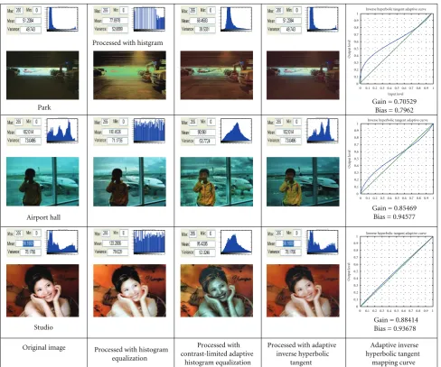
Histgram of processed with AIHT Park

Processed with histgram

Studio

Original image _P_r_{ocessed with histo}_gr_am equalization

tangent

mapping curve Gain = 0.88414 Bias = 0.93678

Gain = 0.85469 Bias = 0.94577 Gain = 0.70529

Bias = 0.7962

Airport hall

0 0.1 0.2 0.3 0.4 0.5 0.6 0.7 0.8 0.9 1

Input level

Out

p

ut level

0 0.1 0.2 0.3 0.4 0.5 0.6 0.7 0.80.9 1

0 0.1 0.2 0.3 0.4 0.5 0.6 0.7 0.8 0.9 1 Out p ut level

0 0.1 0.2 0.3 0.4 0.5 0.6 0.7 0.80.9 1

0 0.1 0.2 0.3 0.4 0.5 0.6 0.7 0.8 0.9 1 Out p ut level

limited adaptive histogram equalization, and our method (indoor images).

Specifically, letxbe the gray level of the original image. Then

and the normalized gray levelgcan be obtained by

g= x−min(x)

max(x)−min(x), (4)

where min(x) and max(x) represent the minimum and maximum gray levels in original image, respectively. Having

implemented AIHT,gis mapped togusing

g=Ta,b,g, (5)

where T indicates an AIHT transform, a andb represent

parameters to be adjusted. Ifx is a gray level of enhanced

image, thenxcan be expressed as

x=(max(x)−min(x))g+ min(x). (6)

Figure 7shows a block diagram of the AIHT algorithm.

The input data is converted from its original format to a floating point representation of RGB values. The principal characteristic of our proposed enhancement function is an adaptive adjustment of the Inverse Hyperbolic Tangent (IHT) Function determined by each pixel’s radiance. After reading the image file, the bias(x) and gain(x) are computed. These parameters control the shape of the IHT function.

Figure 8shows a block diagram of AIHT parameters

eval-uates, including bias(x) and gain(x) parameters.

(14)

0 0.1 0.2 0.3 0.4 0.5 0.6 0.7 0.80.9 1 0 0.1 0.2 0.3 0.4 0.5 0.6 0.7 0.8 0.9 1 Out p ut level

0 0.1 0.2 0.3 0.4 0.5 0.6 0.7 0.80.9 1

0 0.1 0.2 0.3 0.4 0.5 0.6 0.7 0.8 0.9 1 Out p ut level

0 0.1 0.2 0.3 0.4 0.5 0.6 0.7 0.80.9 1

0 0.1 0.2 0.3 0.4 0.5 0.6 0.7 0.8 0.9 1 Out p ut level

00.10.20.30.40.50.60.70.80.91 0 1 2 3 4 5 6 7

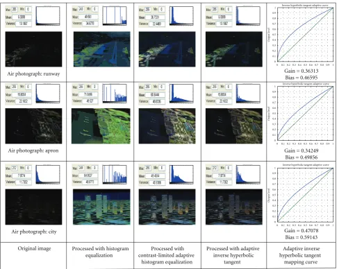
Airphotograph: runway

00.10.20.30.40.50.60.70.80.91 0 1 2 3 4 5 6 7 8 0 0.5 1 1.5 2 2.5 3

00.10.20.30.40.50.60.70.80.91 00.10.20.30.40.50.60.70.80.91 0 1 2 3 4 5 6 7

00.10.20.30.40.50.60.70.80.91 0 1 2 3 4 5 6

Airphotograph: apron

00.10.20.30.40.50.60.70.80.91 0 1 2 3 4 5 6 0 0.5 1 1.5 2 2.5

00.10.20.30.40.50.60.70.80.91 00.10.20.30.40.50.60.70.80.91 0 1 2 3 4 5

00.10.20.30.40.50.60.70.80.91 0 1 2 3 4 5

Airphotograph: city

00.10.20.30.40.50.60.70.80.91 0 1 2 3 4 5 6 0 0.5 1 1.5 2 2.5

00.10.20.30.40.50.60.70.80.91 00.10.20.30.40.50.60.70.80.91 0 0.5 1 1.5 2 2.5 3 3.5 4 4.5 5

Original image Processed with histogram equalization

tangent

mapping curve Gain = 0.36313 Bias = 0.46595

Gain = 0.34249 Bias = 0.49856

Gain = 0.47078

Bias = 0.59143

×104

×104 Histgram of original image Histgram of processed with histgram Histgram of processed with AIHT

Histgram of original image Histgram of processed with histgram Histgram of processed with AIHT

×104 ×104

×104

limited adaptive histogram equalization, and our method (aerial images).

advantage of this function is that it supports an approxi-mately inverse hyperbolic tangent mapping for intermediate luminance, or luminance distributed between dark and

bright values.Figure 9shows an example where the middle

section of the curve is approximately linear.

The form of the AIHT fits data obtained from measuring the electrical response of photo-receptors to flashes of light in

various species [18]. It has also provided a good fit to other

electro-physiological and psychophysical measurements of

human visual function [19–21].

The contrast of an image can be enhanced using inverse hyperbolic function by

tanh−1(x)=1

2log

1 +x

1−x

. (7)

Replace the variable x in (7) with xi j, where xi j is the

image gray level of theith row and jth column. We also put

the bias(x) to the power of xi j to speed up the changing.

The gain function is a weighting function which is used to determine the steepness of the AIHT curve. A steeper slope

narrows a smaller range of input values to the display range. The gain function is used to help shape how fast the mid-range of objects in a soft region goes from 0 to 1. A higher gain value means a higher rate in change. The enhanced pixel

xi jis defined as follows:

Enhancexi j

=

⎛ ⎝_log

⎛ ⎝1 +x

bias(x) i j

1−xbias(x)i j ⎞ ⎠₋₁

⎞

⎠_×_gain(x). ₍₈₎

Therefore the steepness of the inverse hyperbolic tangent curve can be further dynamically adjusted.

Figure 10(a)plots the inverse hyperbolic tangent

func-tion over the domain−1< x < 1 with a shift to 0 < x <1

domain inFigure 10(b).

3.2. Bias Power Function. Figure 11 shows that the bias(x) value of the inverse hyperbolic tangent function determines the turning points of the curve. If the bias(x) is greater

than mean = 0.5, then the curve forms a straight line

(15)

Original image

AM 07:30 PM 02:00 PM 10:00

Processed with adaptive inverse hyperbolic tangent

Original image

AM 06:00 PM 01:00 PM 08:00

Original image

AM 04:00 PM 01:00 PM 08:30

Figure19: Capture images at diﬀerent times of the contrast enhancement by our method.

value is mapped to a higher value. A bias(x) value less than

mean = 0.5 shifts the straight-line portion of the inverse

hyperbolic tangent toward lower levels of light.Figure 11(a)

illustrates these relationships where gain(x)=0.5. Similarly,

a family of inverse hyperbolic tangent remapping curves can be generated by having the bias(x) parameter fixed such as

at mean=0.5 and varying the gain(x) parameter as shown

in Figure 11(b). Decreasing the gain(x) value increases the

contrast of the remapped image. Shifting the distribution toward lower levels of light (i.e., decreasing bias(x)) decreases the highlights. By adjusting the bias(x) and gain(x), it is possible to tailor a remapping function with appropriate amounts of image contrast enhancement, highlights, and

(16)

1 0.8 0.6 0.4 0.2 0 0 1 2 3 4 5 6 ×104

1 0.8 0.6 0.4 0.2 0 0 0.5 1 1.25 2.35 3.45 4.55

×104

1 0.8 0.6 0.4 0.2 0 0 1 2 3 4 5 6 ×104

Original histogram

Histogram after map with AIHT

Processed with histogram equalization of histogram Histogram shape change

Blocking eﬀect

Edge is un-smooth

Details missing

Chromatic aberration

Figure20: Histogram equalization problems.

To make the inverse hyperbolic tangent curve produce a

smooth mapping, we rely on Perlin and Hoﬀert “bias”

func-tion [22]. Bias was first presented as a density modulation

function to change the density of the soft boundary between the inside and the outside of a procedural hyper texture. It is a standard tool in texture synthesis and is also used for

many diﬀerent computer graphics tasks. The bias function

is a power function defined over the unit interval which

remapsx according to the bias transfer function. The bias

function is used to bend the density function either upwards or downwards over the [0, 1] interval.

The bias power function is defined by

bias(x)=

mean(x) 0.5

0.25

=

(1/(m×n))mi=1

n j=1xi j

0.5

0.25

.

(9)

(17)

Original image

(a)

Bias=0.6 processed of image

(b)

(c) Bias=1 processed of image

(d)

(e)

(f) Bias=1.6 processed of image

(g)

(h)

Bias=2 processed of image

(i)

Figure21: (a) is a bad contrast image, (b)–(i) illustrate results using the proposed method with diﬀerent factors, yielding diﬀerent scales of

enhanced image details.

3.3. Gain Function. The gain function determines the steep-ness of the AIHT curve. A steeper slope maps a smaller range of input values to the display range. The gain function is used to help to reshape the object’s midrange from 0 to 1 of its soft region.

The gain function is defined by

gain(x)=0.1×(variance(x))0.5

=0.1× ⎛ ⎝ 1

m×n

m

i=1 n

j=1

xi j−μ ⎞

⎠ 0.5

, (10)

where

μ= 1

m×n

m

i=1 n

j=1

xi j. (11)

Figure 13shows the gain curve for diﬀerent mean values.

The gain function determines the steepness of the AIHT curve.

Figure 14shows the gain curve for diﬀerent gain values

of mapping curves and processed images. There are a total of eight gain values (1, 0.99, 0.97, 0.93, 0.85, 0.69, 0.37),

mapping curves as shown inFigure 14(a). The

correspond-ing results are shown inFigure 14(b).

Figure 15shows processed images and the bias curve for

diﬀerent bias values used by mapping curves. There are a

total of nine bias values (0.4, 0.5, 0.65, 0.8, 1.0, 1.25, 1.6,

2.1, 2.8), mapping curves as shown in Figure 15(a). The

corresponding results are shown inFigure 15(b).

4. Implementation and Experimental Results

Images with diﬀerent types of histogram distributions were

tested for experiments. These include some daily life images that may arise in contrast to the poor image and demonstrate the enhanced results. The images are categorized into out-door, inout-door, and aerial images. The outdoor images include dawn, afternoon, and night images. The indoor images include park, hall, and studio images. The aerial images include runway, apron, and city images. There are four types of extreme images: dark image, bright image, back-lighted

image, and low-contrast image. Figures16,17, and18show

various types of images with bad contrast enhancement.

Figures 16, 17, and 18 display the results of the enhanced

image processing by histogram equalization, contrast limited adaptive histogram equalization, and the proposed AIHT

method. Figures16–18show outdoor images, indoor images,

and aerial images, respectively. Table 1 lists the values of

gain and bias parameters used for the AIHT method.Table 2

compares results by histogram equalization, contrast limited adaptive histogram equalization with that produced by the AIHT method using the measures of MSE, SNR, and PSNR, where the AIHT method was better than histogram equalization and contrast limited adaptive histogram equal-ization.

The comparative analysis between the proposed methods and currently frequently used methods has showed the

(18)

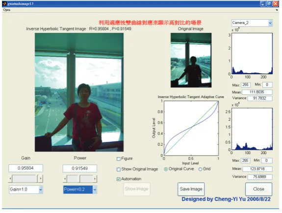
(a)

(b)

Figure22: The user interface of the AIHT system: (a) automatic mode, (b) manual mode.

Table1: Gain and bias parameters.

Type Name Gain Bias

Outdoor images

Dawn 0.684 1.149

Afternoon 0.944 1.026

Night 0.396 0.632

Indoor images

Park 0.705 0.796

Hall 0.855 0.946

Studio 0.884 0.937

Aerial images

Runway 0.363 0.466

City 0.342 0.499

Apron 0.470 0.591

contrast of the poor images. The AIHT technique can keep the sharpness of defects’ edges well. Therefore, CLAHE and AIHT can greatly enhance poor image and they will be helpful for defect recognition.

Figure 19 shows images captured at diﬀerent times of

the contrast enhancement by the AIHT method. Comparing these ongoing processing results, we can see that his-togram equalization and contrast limited adaptive hishis-togram equalization produces grave chromatic aberration, blocking

eﬀects, missing details, rough edges. Furthermore, there is

also a histogram shape change issue as well (Figure 20).

Our approach has no chromatic aberration, blocking eﬀects,

(19)

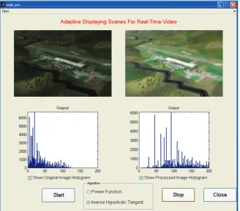
Figure23: Enhancing the real-time image using the AIHT system.

Table2: MSE, SNR, and PSNR.

Type Name Adaptive inverse hyperbolic tangent Histogram equalization

Contrast limited adaptive histogram equalization

MSE SNR PSNR MSE SNR PSNR MSE SNR PSNR

Outdoor images

Dawn 0.0386 22.1137 25.8902 0.16913 5.0272 5.9127 0.0432 10.316 23.143 Afternoon 0.0099 45.0963 101.170 0.00961 46.391 104.08 0.0432 10.316 23.143 Night 0.0174 0.85413 57.3469 0.16739 0.0890 5.9741 0.0596 0.2499 16.780

Indoor images

Park 0.0034 28.8848 295.286 0.05862 1.6688 17.060 0.0339 2.8852 29.495 Hall 0.0163 22.1386 61.4400 0.00206 175.15 486.08 0.0492 7.3229 20.323 Studio 0.0157 21.0555 63.6445 0.02702 12.245 37.013 0.0561 5.8972 17.825

Aerial images

Runway 0.0125 1.78040 79.7332 0.07680 0.0533 13.021 0.0369 0.1109 27.098 City 0.0214 0.18545 46.6504 0.11459 0.0347 8.7265 0.0575 0.0691 17.381 Apron 0.0125 1.07540 80.3171 0.12156 0.1102 8.2265 0.0585 0.2289 17.098

Finally,Figure 21demonstrates the multiscale property

of the AIHT method. The original image (Figure 21(a))

has bad contrast. Figures 21(b)–21(i) presents the results

produced by the AIHT method using diﬀerent factors to yield

diﬀerent scales of enhanced image details.Figure 22shows

the AIHT system interface in manual and automatic mode.

The automatic mode adjusts the best parameters (gainand

bias) based on the automatic calculation of characteristics of

images (meanandvariance) (Figure 22(a)). In manual mode,

users can select their own personal preference to adjust

the parameters (Figure 22(b)). The AIHT method can also

adjust the contrast of real-time-processed images as shown

inFigure 23.

5. Conclusions

This paper presents an eﬀective approach to image contrast

enhancement. The proposed algorithm uses an Adaptive Inverse Hyperbolic Tangent algorithm as a contrast function to map from the original image into a transformed image. This algorithm can improve the displayed quality of contrast

(20)

Experimental results show that it is possible to maintain a large portion, if not all, of the perceived contrast of lightness while enhancing the image contrast significantly. The form of these curves used for enhancement was determined based on a simple series of interpolations from a set of optimized reference curves. The proposed algorithm can make the user correctly identify the target as well as dynamically adjust the parameter by using the multiscale method. Experimental results also show that the new algorithm can adaptively enhance image contrast and produce better visual quality than histogram equalization and contrast-limited adaptive histogram equalization. In addition, it can also be implemented in real time in various monitor systems. For overexposed and underexposed images the proposed algorithm also shows great benefit in improving contrast

enhancement with no eﬀects resulting from environments.

It is our belief that these functions will play a crucial role in developing a more universal approach to color gamut mapping.

Acknowledgments

This work was supported by National Science Council (NSC) of Taiwan, R.O.C. (NSC 98-2221-E-005-064).

References

[1] Y. Monobe, H. Yamashita, T. Kurosawa, and H. Kotera, “Dynamic range compression preserving local image contrast for digital video camera,” IEEE Transactions on Consumer

Electronics, vol. 51, no. 1, pp. 1–10, 2005.

[2] F. A. Dunn, M. J. Lankheet, and F. Rieke, “Light adaptation in cone vision involves switching between receptor and post-receptor sites,”Nature, vol. 449, no. 7162, pp. 603–606, 2007. [3] G. Osterberg, “Topography of the layer of rods and cones in

the human retina,”Acta Ophthalmologica, vol. 13, supplement 6, pp. 1–103, 1935.

[4] C. Y. Yu, Y. Y. Chang, T. W. Yu, Y. C. Chen, and D. Y. Jiang, “A local-based adaptive adjustment algorithm for digital images,”

inProceedings of the 2nd Cross-Strait Technology, Humanity

Education and Academy-Industry Cooperation Conference, pp.

637–643, 2008.

[5] T. W. Yu, S. S. Su, C. Y. Yu, C. Y. Lin, and Y. Y. Chang, “Adaptive displaying scenes for real-time image,” inProceedings of the 3rd

Intelligent Living Technology Conference, pp. 731–737, 2008.

[6] Z. Wang, A. C. Bovik, H. R. Sheikh, and E. P. Simoncelli, “Image quality assessment: from error visibility to structural similarity,”IEEE Transactions on Image Processing, vol. 13, no. 4, pp. 600–612, 2004.

[7] D. Garvey, “Perceptual strategies for purposive vision,” Tech-nical Note 117, AI Center, SRI International, 1976.

[8] C. Y. Yu, Y. C. Ouyang, C. M. Wang, C. I. Chang, and Z. W. Yu, “Contrast adjustment in displaying scenes using inverse hyperbolic function,” inProceedings of the 22th IPPR

Confer-ence on Computer Vision, Graphics, and Image Processing, pp.

1020–1027, 2009.

[9] R. C. Gonzalez and R. E. Woods, “Digital Image Processing,” Prentice Hall, Upper Saddle River, NJ, USA, 3rd edition, 2008. [10] ERDAS, Inc., Overview of ERDAS IMAGINE 8.2, ERDAS,

Atlanta, Ga, USA, 1995.

[11] J. Duan and G. Qiu, “Novel histogram processing for colour image enhancement,” inProceedings of the 3rd International

Conference on Image and Graphics (ICIG ’04), pp. 18–22, Hong

Kong, December 2004.

[12] J. Rosenman, C. A. Roe, R. Cromartie, K. E. Muller, and S. M. Pizer, “Portal film enhancement: technique and clinical utility,” International Journal of Radiation Oncology Biology

Physics, vol. 25, no. 2, pp. 333–338, 1993.

[13] K. Zuiderveld, “Contrast limited adaptive histogram equaliza-tion,” inGraphics Gems IV, P. S. Heckbert, Ed., chapter 8.5, pp. 474–485, Academic Press, Cambridge, Mass, USA, 1994. [14] T. G. Stockham, “Image processing in the context of a visual

model,”Proceedings of the IEEE, vol. 60, no. 7, pp. 828–842, 1972.

[15] F. Drago, K. Myszkowski, T. Annen, and N. Chiba, “Adaptive logarithmic mapping for displaying high contrast scenes,” in

Proceedings of European Association for Computer Graphics

24th Annual Conference (EUROGRAPHICS ’03), vol. 22, pp.

419–426, Granada, Spain, September 2003.

[16] E. P. Bennett and L. McMillan, “Video enhancement using per-pixel virtual exposures,”ACM Transactions on Graphics, vol. 24, no. 3, pp. 845–852, 2005, ACM SIGGRAPH 2005 Paper SIGGRAPH ’05.

[17] P. Whittle, “Increments and decrements: luminance discrimi-nation,”Vision Research, vol. 26, no. 10, pp. 1677–1691, 1986. [18] K. I. Naka and W. A. Rushton, “S-potentials from luminosity units in the retina of fish (cyprinidae),”Journal of Physiology, vol. 185, no. 3, pp. 587–599, 1966.

[19] J. Kleinschmidt and J. E. Dowling, “Intracellular recordings from gecko photoreceptors during light and dark adaptation,”

Journal of General Physiology, vol. 66, no. 5, pp. 617–648, 1975.

[20] D. C. Hood and M. A. Finkelstein, “A comparison of changes in sensitivity and sensation: implications for the response-intensity function of the human photopic system,”Journal of

Experimental Psychology: Human Perception and Performance,

vol. 5, no. 3, pp. 391–405, 1979.

[21] D. C. Hood, M. A. Finkelstein, and E. Buckingham, “Psy-chophysical tests of models of the response function,”Vision

Research, vol. 19, no. 4, pp. 401–406, 1979.

[22] K. Perlin and E. M. Hoﬀert, “Hypertexture,”ACM SIGGRAPH

Computer Graphics, vol. 23, no. 3, pp. 253–262, 1989,