Research Article
A Forward-Backward Kalman Filter-based
STBC MIMO
OFDM
Receiver
T. Y. Al-Naffouri and A. A. Quadeer
Electrical Engineering Department, King Fahd University of Petroleum and Minerals, Dhahran 31261, Saudi Arabia
Correspondence should be addressed to A. A. Quadeer,[email protected]
Received 5 May 2008; Accepted 11 December 2008
Recommended by Kostas Berberidis
Orthogonal frequency division multiplexing (OFDM) has emerged as a modulation scheme that can achieve high data rates over frequency selective fading channel by efficiently handling multipath effects. This paper proposes receiver design for space-time block codedMIMO OFDMtransmission over frequency selective time-variant channels. Joint channel and data recovery are performed at the receiver by utilizing the expectation-maximization (EM) algorithm. It makes collective use of the data constraints (pilots, cyclic prefix, the finite alphabet constraint, and space-time block coding) and channel constraints (finite delay spread, frequency and time correlation, and transmit and receive correlation) to implement an effective receiver. The channel estimation part of the receiver boils down to anEM-based forward-backward Kalman filter. A forward-only Kalman filter is also proposed to avoid the latency involved in estimation. Simulation results show that the proposed receiver outperforms other least-squares-based iterative receivers.
Copyright © 2008 T. Y. Al-Naffouri and A. A. Quadeer. This is an open access article distributed under the Creative Commons Attribution License, which permits unrestricted use, distribution, and reproduction in any medium, provided the original work is properly cited.
1. INTRODUCTION
Orthogonal frequency division multiplexing (OFDM) is a technique that enables high speed transmission over fre-quency selective channels with simple equalizers. It does this by creating a set of parallel frequency-flat channels over which large constellation signals can be transmitted. For frequency flat fading channels, space-time codes provide diversity and coding gain benefits compared with single-input single-output (SISO) systems improving theBER per-formance of the system [1]. (We concentrate in this work on space-frequency codes. We note however that a very similar approach can be used for space-time block codes (STBC). Given the similarity between the two approaches and the fact that the abbreviationSTBCis more familiar, we continue to use this abbreviation to refer to our frequency-space codes.) When multiple antennas (MIMO) are combined withOFDM, space-time codes can be used per tone, providing the benefit of multiple antennas with simple channel equalization.
AnOFDMreceiver needs channel state information (CSI) to detect the data. With no CSI at the receiver, both the channel and the data are unknowns that have to be recovered. The estimation process can be carried out jointly
1.1. Paper contributions
This paper considers receiver design forOSTBC-OFDM trans-mission over a frequency selective, time-variant channel. We propose a semiblind iterative receiver using theEMalgorithm for joint channel and data recovery. The main contributions of the work are summarized below.
(1) We make a collective use of the structure of the communication problem (i.e., the constraints on the data and on the channel) in a transparent manner. The data constraints include the finite alphabet constraint [13], the cyclic prefix [8], pilots [6,7], and theOSTBC. In addition, the receiver uses the following constraints on the channel: the finite delay spread, frequency and time correlation [22–24], and spatial correlation (it is also straightforward to incorporate channel sparsity [15, 25, 26]). This is in contrast to the work done by other researchers as none has used all the above mentioned constraints in such a collective and transparent manner.
(2) The channel estimation and data detection as well as the exploitation of the system constraints is done in a semioptimal manner through theEMalgorithm. This guarantees a simple receiver structure.
(3) In spite of the complexity of the problem that we address here and the many constraints we incorpo-rate, our algorithm maintains its transparency:
(a) the maximization step is used for channel estimation and makes use of the channel constraints by employing a forward-backward Kalman filter.
(b) the expectation step is used for data detection and makes use of the data constraints.
(4) In contrast to prior approaches, we take a channel estimation centric viewpoint and reverse the roles of the channel and the transmitted signal in our implementation of theEMalgorithm [19] using the estimation step for data detection and maximization step for channel estimation. We do so because it is difficult to employ the expectation step for channel estimation while simultaneously incorporating the various constraints on the channel (most notably, the time-correlation constraint).
A similar algorithm was proposed by the first author in [27] for theSISOcase. Extending this algorithm to the
MIMO case is nontrivial. For in addition to the scale up in the number of transmit and receive antennas, this paper (1) makes use of the space-time code and (2) makes full use of the frequency and time correlation as well as transmit and receive spatial correlation (see Section 2.2andAppendix A
where we derive the channel model). Moreover, and in spite of the many dimensions we deal with, we maintain the transparency of the presentation.
1.2. Paper organization
The paper is organized as follows. After introducing our notation, we give an overview of the transceiver inSection 2.
Section 3 then derives the input/output (I/O) equations
for MIMO-OFDM with STcoding (the equations are needed for channel and data recovery). Channel estimation using the forward-backward (FB) Kalman filter is derived in
Section 4at the end of which we summarize the transceiver
algorithm with an extension/modification of the algorithm.
Section 5 presents our simulations and Section 6 presents
our conclusions.
1.3. Notation
Proper choice of notation is essential for clarity and con-sistency. One challenge in choosing notation is the many dimensions we deal with in this paper including sample time, (frequency) tone, (channel) tap, (OFDM) symbol index, and space.
In this paper, we denote scalars with small-case letters (e.g., x), vectors with small-case boldface letters (e.g., x), and matrices with uppercase boldface letters (e.g., X). Calligraphic notation (e.g.,X) is reserved for vectors in the frequency domain. A hat over a variable indicates an estimate of the variable (e.g.,his an estimate ofh). We use∗to denote conjugate transpose,⊗to denote Kronecker product,IN to
denote the sizeN×Nidentity matrix, and0M×N to denote
the all zeroM×Nmatrix. Given a sequence of vectorshtx
rx
forrx =1· · ·Rxandtx =1· · ·Tx, we define the following
stack variables:
hrx=
⎡ ⎢ ⎢ ⎢ ⎣
h1
rx
.. .
hTx
rx
⎤ ⎥ ⎥ ⎥
⎦, h=
⎡ ⎢ ⎢ ⎣
h1 .. .
hRx
⎤ ⎥ ⎥
⎦. (1)
The notation vec(X) denotes a column vector consisting of the concatenation of all column vectors of X while the operation diag(X) transforms the vectorX into a matrix with diagonalX.
2. AN OVERVIEW OF THE COMMUNICATION SYSTEM
In this section, we give an overview of the communications system: transmitter, channel, and receiver.
2.1. Transmitter
Pilot
insert. encodeSTBC r
IFFT
IFFT
IFFT
Cyclic
prefix
Cyclic
prefix
Cyclic
prefix
Puncturer
Encoder Interleaver Modulator
Figure1:OSTBC OFDMtransmitter.
symbols to construct theSTblock by mapping the various
OFDM symbols to a specific antenna and specific time slot depending on theSTcode used. Each antenna performs an
IFFToperation on theOFDM symbols to produce the time-domainOFDMsymbols and adds a cyclic prefix to each prior to transmission.
2.2. Channel model
We consider a time-variant and frequency selective MIMO channel. For a general MIMO system, theI/Otime-domain relationship is described by
y(m)=
P
p=0
H(p)x(m−p), (2)
where H(p) is the Rx×Tx MIMO impulse response at tap
p and wheremrepresents the sample time index. The taps
H(p) usually incorporate the effect of the transmit filter and the effects of the transmit and receive correlation making
H(p) correlated across space and tap. We will assume for simplicity that H(p) is iid for all p (In Appendix A we consider the general case where the channel exhibits transmit and receive correlation). We will also assume that the tap
H(p) remains constant over a single STblock (and hence over the constituent OFDM symbols) and changes from the current block (Ht(p)) to the next (Ht+1(p)) according to the dynamical equation (We will at times suppress the time dependence for notational convenience.)
Ht+1(p)=α(p)Ht(p) +
(1−α2(p))e−βpU
t(p). (3)
Here,Ut(p) is an iid matrix with entries that are N(0, 1),
and α(p) is related to the Doppler frequency fD(p) by
α(p)=J0(2π fD(p)T), whereTis the time duration of oneST
block. The variableβin (3) corresponds to the exponent of the channel decay profile while the factor
(1−α2(p))e−βp
ensures that each link maintains the exponential decay profile (e−βp) for all time.
This channel model allows the channel to be time variant (as the channel can change arbitrarily from one ST block to the next) while avoiding intercarrier interference and ensuring the proper operation of the space-time code (as the channel remains fixed over any one OFDM symbol or
ST block). This model was adopted in [23,28,29] in an
SISO context. (This model is based on approximating the nonrational Jakes model by a first-orderARmodel. It is also possible to have a better approximation by employing higher-orderARmodels but this would increase the latency of the receiver.)
In this paper, we scale up the model to theMIMO case and also show how to incorporate transmit and receive correlation in Appendix A (see [27, 30] where we also incorporate the effect of the receive filter).
Using this dynamical model, we can obtain the state-space model for the impulse responsehtx
rxbetween transmit
antennatxand receive antennarx. From (3), we can write
htx
rx,t+1(p)=α(p)h
tx
rx,t(p) +
1−α2(p)e−βputx
rx,t(p). (4)
By stacking (4) over the taps p = 0, 1,. . .,P, we obtain the dynamical model
htx
rx,t+1=Fh
tx
rx,t+Gu
tx
rx,t, (5)
where
F= ⎡ ⎢ ⎢ ⎣
α(0) . ..
α(P)
⎤ ⎥ ⎥ ⎦,
G=
⎡ ⎢ ⎢ ⎢ ⎣
1−α2(0) . ..
1−α2(P)e−βP ⎤ ⎥ ⎥ ⎥ ⎦.
(6)
By further stacking (5) over all transmit and receive antennas (refer to our stacking notation in (1)), we obtain
ht+1=
ITxRx⊗F
ht+
ITxRx⊗G
ut, (7)
whereht+1,ht, andut, are vectors of sizeTxRx(P+ 1)×1.The
dynamical equation (7) shows explicit dependence on the space-time indext(sot=1 for the first space-time symbol which consists of twoOFDM symbols in the Alamouti case, t=2 for the second space-time symbol, etc.).
covariance of the channel at the first time instant. It is easy to show that
Eutu∗t
=IRx⊗E
urxu∗rx
=IRx⊗
ITx⊗E
utx
rxu
tx∗
rx
=IRx⊗ITx⊗IP+1=ITxRx(P+1).
(8)
We can similarly show that the channel covariance at the first time instant is given by
Eh0h∗0
=ITxRx⊗GG∗. (9)
The covariance information is important for employing the Kalman filter which is used for channel estimation. We finally note that while (3) and (7) are equivalent, the latter model is in vector form and hence lends itself more to the Kalman filter operations, which are used for channel estimation.
A note about time variation
One drawback of the approach in this paper is the block fading model that we adopt. For it is more realistic to assume that the channel continuously varies with time. There are 3 justifications for using the block fading model.
(1) While it is more realistic to assume that the channel continuously varies over theOFDMsymbol, the model we assume is more valid than the block-fading model that is widely used in literature. For in the block-fading model, it is usually assumed that the channel remains constant over any one symbol and varies independentlyfrom one symbol to another. Here, we account for the time correlation across symbols. (2) The purpose of this paper is to design an algorithm
that makes a collective use of the underlying structure of the communication problem to lower the training overhead required in the time-variant case. Solving the general time-variant case is a future research problem that builds upon the findings in this paper [31].
(3) One could still envision applications where the channel is constant over an ST block, but varies substantially from one symbol to the next. Consider, for example, a multiuser application in which the wireless channel is time shared. Imagine also that the channel is very slowly time variant but the duty cycle is very large. In that case, the channel that each user experiences during his transmission burst is very slow, but from one burst to another, the channel would change substantially due to the long duty cycle. This situation would also make sense in random access scenarios.
2.3. Receiver
This paper is concerned with designing a receiver for the system described above. For completeness and as an allusion to the developments further ahead,Figure 2shows a block diagram of the proposed receiver. As we will show, the receiver’s core operation is based on theEMalgorithm which performs joint channel and data recovery.
2.3.1. STBCdecoder/data detector (estimation step)
The STBC decoder/data detector calculates the conditional first and second moments of the transmitted data (soft estimate) to be used by the channel estimator.
2.3.2. channel estimator (maximization step)
Pilots are used to initialize channel estimation. The channel estimator then uses the soft data estimates together with the data and channel constraints to improve the channel estimate. These two processes (channel estimation and data detection) go on iteratively until a stopping criterion is satisfied.
3. INPUT/OUTPUT EQUATIONS FORMIMO-OFDM
As pointed out in Section 2.3, the receiver performs two operations, channel estimation and data detection. As such, we need to derive two forms of theI/Oequations: one that lends itself to channel estimation (i.e., treats the channel impulse response as the unknown) and a dual version that lends itself to data detection (i.e., treats the input in its uncoded form as the unknown). To this end, let Xtx be
theOFDMsymbol transmitted through antennatxwhich first
undergoes an IDFT xtx = 1/NQXtx where Q is the N ×
N IDFT matrix. The system then appends a cyclic prefix before transmission. At the receiver end, the receiver strips the cyclic prefix to obtain the time domain symbolytx
rx.The
I/Oequation of theOFDMsystem between transmit antenna txand receive antennarx is best described in the frequency
domain
Ytx
rx=diag(Xtx)Q∗P+1htrxx+Nrx, (10)
where Ytx
rx,Xtx,H
tx
rx, and N
tx
rx are the (length-N)DFTs of
ytx
rx,xtx,h
tx
rx,nrx, respectively, and where (10) follows from the
fact that
Htx
rx =Q
∗
htx
rx
O(N−P−1)×1
=Q∗P+1htrxx. (11)
Here, QP+1 represents the first P + 1 rows of Q. By superposition and using the stacking notation (1), we can express theI/Oequation at receive antennarxas
Yrx=
diagX1
· · ·diagXTx
ITx⊗Q∗P+1
hrx+Nrx.
(12)
3.1. I/Oequations: channel estimation version
Consider a set of Nu uncoded OFDM symbols {S(1),. . .,
S(Nu)} which we would like to transmit over Tx
anten-nas and Nc time slots. Following [32], we can
per-form ST coding using the set of Tx × Nc matrices
{A(1),B(1),. . .,A(Nu),B(Nu)} which characterizes the ST
code. We can now show that theOFDM symbol transmitted from antennatxat timencis given by [32]:
Xtx
nc
=
Nu
nu=1
atx,nc
nu
ReSnu
+jbtx,nc
nu
ImSnu
,
Cyclic
prefix removal
Cyclic
prefix removal
Cyclic
prefix removal
STBC
decoder removalPilot modulatoDe- r
De-interleaver punctuDe-rer Decoder
Initial channel estimator FFT FFT FFT Channel estimator
E[X] E[X2] hest
hest, final hest, initial
Figure2:OSTBC OFDMreceiver.
whereatx,nc(nu) is the (tx,nc) element ofA(nu) andbtx,nc(nu)
is the (tx,nc) element ofB(nu). Thus, in the presence ofST
coding, (12) reads Yrx
nc
=diagX1
nc
· · ·diagXTx
nc
×ITx⊗Q
∗
P+1
hrx+Nrx
nc
. (14)
(It should be clear that by using anSTcode, a diversity ofTx×
Rx is achieved by spreading each symbol in time and space
at the transmitter antenna. The symbols are not spread in frequency and thus, (multipath) diversity is lost at the price of decoding simplicity (i.e., bin by bin decoupling).) This represents theI/Oequation at antennarxatOFDMsymbolnc
of anSTblock. Collecting this equation for all such symbols yields
Yrx=Xhrx+Nrx, (15)
where
Yrx=
⎡ ⎢ ⎢ ⎣
Yrx(1)
.. . Yrx(Nc
⎤ ⎥ ⎥ ⎦, X= ⎡ ⎢ ⎢ ⎢ ⎢ ⎣
diagX1(1)
· · ·diagXTx(1)
ITx⊗Q
∗
P+1
diagX1(2)
· · ·diagXTx(2)
ITx⊗Q∗P+1
.. .
diagX1
Nc
· · ·diagXTx
Nc
ITx⊗Q
∗ P+1 ⎤ ⎥ ⎥ ⎥ ⎥ ⎦. (16)
Now, by further collecting this relationship over all receive antennas, we obtain
Yt=
IRx⊗Xt
ht+Nt. (17)
This equation captures theI/Orelationship atallfrequency bins, for all input and output antennas, and for all OFDM symbols of thetthSTblock.
To perform initial channel estimation, we select those equations where the pilots are present. Let Ip denote the
index set of the pilots bins. Then, the pilot/output equation takes the form
YtIp=
IRx⊗XtIp
ht+NtIp. (18)
As can be seen, (17) and (18) are quite similar and using them in a Kalman filter context will be similar as well.
3.2. I/Oequations: data detection version
Signal detection inST-codedOFDMis done on a tone-by-tone basis (as inSISO OFDM), except that the tones are collected for the wholeSTblock (i.e., forRxreceive antennas and over
Nctime slots). From (10), we can construct the followingI/O
equationat any tonenbelonging to theOFDMsymbolnc:
Yrx
nc
=H1
rx · · · H
Tx rx ⎡ ⎢ ⎢ ⎣ X1 nc .. . XTx
nc ⎤ ⎥ ⎥ ⎦+Nrx
nc
.
(19)
We suppress the dependence on n for notational conve-nience. Collecting this relationship for all receive antennas yields ⎡ ⎢ ⎢ ⎣ Y1 nc .. . YRx
nc ⎤ ⎥ ⎥ ⎦= ⎡ ⎢ ⎢ ⎣ H1
1 · · · H
Tx
1 ..
. · · · ... H1
Rx · · · H
Tx Rx ⎤ ⎥ ⎥ ⎦ ⎡ ⎢ ⎢ ⎣ X1 nc .. . XTx
nc ⎤ ⎥ ⎥ ⎦+ ⎡ ⎢ ⎢ ⎣ N1 nc .. . NRx
nc ⎤ ⎥ ⎥ ⎦, (20)
or, more succinctly,
Y(nc)=HX(nc) +N(nc). (21)
By further concatenating this relationship fornc=1,. . .,Nc,
we can show that the following relationship holds (see [32]):
Y=C
ReS ImS
+N, (22)
where Y= ⎡ ⎢ ⎢ ⎣ Y(1) .. . Y(Nc)
⎤ ⎥ ⎥
⎦, S=
⎡ ⎢ ⎢ ⎣ S(1) .. . S(Nu)
⎤ ⎥ ⎥
⎦, C=Ca Cb
,
with Ca = [ vec(HA(1)) · · · vec(HA(Nu)) ] and Cb =
[ vec(HB(1)) · · · vec(HB(Nu)) ].We finally note that the
STBCcode is orthogonal if and only if the matrixCsatisfies [32]
Re[C∗C]= H2
I2Nu ∀H. (24)
This property is essential to perform data detection. We stress that the relationships (19) through (24) apply at a particular tonenand that this dependence has been omitted for notational convenience.
4. JOINT CHANNEL AND DATA ESTIMATION: ANEMAPPROACH
4.1. TheEMalgorithm
Consider theI/Oequation (17) reproduced here for conve-nience
Yt=
IRx⊗Xt
ht+Nt. (25)
Ideally, we estimate ht by maximizing some log-likelihood
function, for example,
hMAPt =max
ht
lnpYt|Xt,ht
+ lnpht
. (26)
In our case, however, the inputXtis not available. Thus, we
use theEMalgorithm and maximize instead an averaged form of the log-likelihood function. Specifically, starting from an initial estimateh(0)t , the estimateht is calculated iteratively,
with the estimate at thejth iteration given by
h(tj)=arg max ht
EX
t|Yt,h
(j−1)
t lnp
Yt|Xt,ht
+ lnpht
.
(27)
For example, when the system obeys theI/Orelationship (25) andhtisN(0,Π), theEM-based estimate (at thejth iteration)
is given by
h(tj)=arg min ht
Yt−
IRx⊗E
Xt
ht21/σ2
n
+ht2I⊗Cov[X∗t]+ht
2 Π−1,
(28)
where the two moments ofXtare taken given the outputYt
and the most recent channel estimateh(tj−1).(The weighted
norm notationh2
Astands forh∗Ah.) We now derive theEM
algorithm for the time-variant case.
4.2. Channel estimation: anEM-based forward-backward Kalman
Consider theOFDMsystem of this paper, essentially described by the state-space model
ht+1=
ITxRx⊗F
ht+
ITxRx⊗G
ut, (29)
Yt=
IRx⊗Xt
ht+Nt, (30)
withh0 ∼ N(0,Π) andut ∼ N(0,Ru).Given a sequence
ofT+ 1 input and outputSTsymbolsXT
0 andYT0, (we use
XT0 to denote the sequenceX0,X1,. . .,XT) we obtain theMAP
estimate of the channel sequencehT0 by maximizing the log-likelihood
L=lnpYT
0 |XT0,hT0
+ lnphT
0
. (31)
Now, using (30), we can express the first term of the log-likelihood (up to some additive constant) as
lnpYT
0 |XT0,hT0
=
T
t=0
lnpYt|Xt,ht
= −
T
t=0
Yt−
IRx⊗Xt
ht21/σ2
n.
(32)
Similarly, using (29), we can express the second term of (31) (again up to some additive constant) as
lnphT0=
T
t=1
lnpht|ht−1
+ lnph0
= −
T
t=1
ht−
ITxRx⊗F
ht−12(GRuG∗)−1−h0
2 Π−1
0 .
(33)
Combining these two expressions yields
L= −
T
t=1
Yt−
IRx⊗Xt
ht21/σ2
n
−
T
t=1
ht−
ITxRx⊗F
ht−1
2
(GRuG∗)−1−h0
2 Π−1
0 .
(34)
Since the channel sequencehT
0 is jointly Gaussian, the MAP estimate of the channel sequence given the input and output sequencesXT
0 andYT0 is the same as theMMSEestimate given the same sequences. TheMMSEestimate itself is obtained by the forward-backward (FB) Kalman filter. This allows us to state the following theorem. (For a proof, see [33, problem 10.9].)
Theorem 1(channel estimation-known input case). Con-sider the state-space model (29)-(30). Given the input and output sequencesXT0 andYT0,theMAP(or equivalentlyMMSE)
estimate ofhT0 is obtained by applying the following
(forward-backward Kalman) filter to the state-space model(29)-(30).
Forward run
Fori=1,. . .,T,calculate
Re,t=σn2ITxRxN+
IRx⊗Xt
Pt|t−1
IRx⊗X∗t
P0|−1=Π0,
(35)
Kt=Pt|t−1
IRx⊗X
∗
t
R−1
e,t, (36)
ht|t=
ITxRx(P+1)−Kt
IRx⊗Xtht|t−1+KtYt, (37)
ht+1|t=
ITxRx⊗Fht|t, h0|−1=0, (38)
Pt+1|t=(ITxRx⊗F)(Pt|t−1−KtRe,tK∗t)(ITxRx⊗F∗)
+GRuG∗.
Backward run
Starting fromλT+1|T=0and fort=T,T−1,. . ., 0,calculate
λt|T=
IP+N−
IRx⊗X
∗
t
K∗tI⊗F∗λt+1|T
+I⊗Xt
R−1
e,t
Yt−
I⊗Xtht|t−1
, (40)
ht|T=ht|t−1+Pt|t−1λt|T. (41)
The desired estimate isht|T.
(The Kalman filter has been initialized with zero in (38) as we are dealing with Rayleigh channel. For the case of Ricean channel, we only need to initialize the Kalman filter with nonzero mean corresponding to the direct line-of-sight (LOS) signal present in Ricean channel.) This theorem allows us to obtain the estimate of hT
0 when the input sequence XT
0 is not available. For in this case, we maximize the log-likelihood (34)averagedover the sequenceXT0.Thus, thejth iteration of theEMalgorithm is now obtained by maximizing the averaged log-likelihood
L=EXT
0|YT0,h
T(j−1)
0 [L]. (42)
By inspecting (34), we note that the only term that is modified under expectation is the first summand, and its expectation is given by
EYt−
IRx⊗Xt
ht21/2σ2
n
=Yt−
IRx⊗E
Xt
ht21/2σ2
n+
ht2 (1/2σ2
n)IRx⊗Cov[Xt∗]
=
Yt 0TxRx(P+1)×1
−
IRx⊗E
Xt
IRx⊗Cov
X∗t
1/2
ht 2
1/2σ2
n
,
(43)
where the expectations are taken given the previous estimate
h(0j−1)and the output symbolsYT0.We thus have
L= −
T
t=0
Yt 0TxRx(P+1)×1
−
IRx⊗E
Xt
IRx⊗Cov
X∗t
1/2
ht 2
1/2σ2
n
−
T
t=1
ht−Fht−12(GRuG∗)−1−h0
2 Π−1
0 .
(44)
Note that we can obtain the averaged likelihood (44) from the original likelihood (34) by performing the substitution
IRx⊗Xt−→
IRx⊗E
Xt
IRx⊗Cov
X∗t
1/2
,
Yt−→
Yt 0TxRx(P+1)×1
,
(45)
we can thus state the following theorem.
Theorem 2(channel estimation-unknown input case). Con-sider the state-space model (29)-(30) and assume that the receiver does not have access to the transmitted dataXT
0.The
channel estimate at the jth iterationh0 of theEMalgorithm is
obtained by applying the forward-backward Kalman(35)–(41) to the following state-space model
ht+1=
ITxRx⊗F
ht+
ITxRx⊗G
ut, (46)
Yt 0TxRx(P+1)×1
=
IRx⊗E
Xt
IRx⊗Cov
X∗t
1/2
ht+
Nt nt
, (47)
wherentis virtual noise that is not physically present and that is independent of the physical noiseNt.
The virtual noise results from having a norm of the following form: Yt 0TxRx(P+1)×1
−
IRx⊗E
Xt
IRx⊗Cov
X∗t
1/2
ht 2
(1/σ2)I
. (48)
Note that the weighting matrixI is now of size N +P.To account for this, we assume the presence of virtual noisent
which is independent of the actual physical noiseNt in the
I/Oequation (47).
To fully implement theEMalgorithm, we need to initialize the algorithm and calculate the first and second moments of the input, which we do next.
4.3. Initial channel estimation
We obtain the initial channel estimate from the pilot/output equation (18) together with the dynamical channel model (7). Specifically, we do this by applying theFBKalman to the following state-space model
ht+1=
ITxRx⊗F
ht+
ITxRx⊗G
ut, (49)
YtIp =
IRx⊗XtIp
ht+NtIp, (50)
that is, by applying theFBKalman filter (35)–(41) with the following substitution:
Yt−→YtIp, Xt−→XtIp, ITxRxN −→ITxRx|Ip|. (51)
4.4. Data detection
To detect the data, we use the data detection version of the
I/Oequation (22). Upon multiplying both sides byC∗ and taking the real part, we obtain
Y= H2
ReS ImS
+N, (52)
where Y and N are 2Nu ×1 vectors defined by Y =
ReC∗Y and N = ReC∗N. Since C is orthogonal, the noise N remains white, and the input can be detected on an element-by-element basis. (Equation (13) holds for every
conditional pdf f(ReS(nu)|Y(nu),H) by applying Bayes
rule on it which yields
fri|Y
nu
,H= f(ri,Y(nu)|H) f(Y(nu)|H)
=|Rf(|ri,Y(nu)|H)
i=1f(Y(nu),ri|H)
=|Rf(|Y(nu)|ri,H)f(ri|H)
i=1f(Y(nu)|ri,H)f(ri|H)
,
(53)
fri|Y
nu
,H= e
−(|Y(nu)−H2ri|2)/2σn2
|R|
i=1e−(|Y(nu)−H
2r
i|2)/2σn2
. (54)
We can use this pdf to calculate conditional expectation of ReS(nu) and its second moment given the outputY(nu):
EReSnu
|Ynu
,H=
|R|
i=1rie−(|Y(nu)−H 2r
i|2)/2σn2
|R|
i=1e−(|Y(nu)−H
2r
i|2)/2σn2
,
E|ReSnu
|2|Ynu
,H=
|R|
i=1ri2e−(|Y(nu)−H 2r
i|2)/2σn2
|R|
i=1e−(|Y(nu)−H
2r
i|2)/2σn2
.
(55)
We can similarly calculate the two moments of the imaginary part. Now (55), just like (19)–(24), apply at a certain frequency tone n. So collecting (55) for all tones (n = 1,. . .,N) produces the two moments of the uncoded
OFDMsymbols. Specifically, we can calculate
E[ReS(nu)], E[ImS(nu)],
E[diag(ReS(nu))2], E[diag(ImS(nu))2].
(56)
We show inAppendix Bthat these moments are enough to characterize the first and second momentsE[X] andE[X∗X], which are needed for channel estimation.
4.5. Summary of theEM-based receiver
We now have all the elements for the iterative receiver for channel and data recovery, and for ease of reference, we summarize the receiver algorithm in the following. Given a sequence of input and output symbolsXT0 andYT0 perform the following operations.
(1) Calculate the initial channel estimatehT0(0) by apply-ing the FB Kalman filter to the state-space model (49)-(50), that is, by applying (35)–(41) with the following substitutions:
Yt−→YtIp, Xt−→XtIp, ITxRxN −→ITxRx|Ip|.
(57)
(2) Iterate between the expectation and maximization steps forj=1,. . .,Niter:
(a) expectation:
(i) use (55) to compute the first two moments of the uncodedOFDMsymbolsS(1),. . .,S(nu),
given the output YT0 and the most recent estimate of the channel,hT0(j−1);
(ii) use these moments to calculate the moments of
Xthrough the relationships (13) and (55).
(b) maximization:
obtain the channel estimate hT0(j) by employing the FBKalman to the state-space model (46)-(47), that is, by applying (35)–(41) with the following substitutions:
IRx⊗Xt−→
IRx⊗E
Xt
IRx⊗Cov
X∗t
1/2
,
Yt−→
Yt 0TxRx(P+1)×1
,
ITxRxN−→ITxRx(N+P+1).
(58)
The algorithm can be stopped when the maximum number of iterationsNiteris reached or when the difference between two consecutive estimateshT0(j)−h
T(j−1)
0 2is below a certain threshold.
4.6. Modification: Kalman- (forward-only) based estimation
One disadvantage of the FB Kalman (summarized in
Section 4.5above) is the storage and latency involved. The
algorithm needs to wait for all T+ 1STsymbols before it can execute the backward run and hence obtain the channel estimate. One way around this is to reduce the window size T.Alternatively, we can run the filter in the forward direction only (i.e., run (35)–(39)) for both the initial estimation and theEMiteration. The algorithm then collapses to the Kalman-based filter proposed in [34] where the data and channel are recovered within oneSTsymbol.
5. SIMULATION RESULTS
In the following simulations, we test the performance of the forward and forward-backward Kalman filters.
5.1. The forward-only Kalman
The transmitter and receiver illustrated in Figures 1 and
OurMIMO channel model is simulated using the state-space model (7) with parameters,α = 0.985,β = 0.2, and P=7. The number of receive antennas is set toRx=2.
Three thousand packets were simulated perSNR-value. Each packet is comprised of 12 OFDM symbols transmitted over six ST blocks. Each OFDM symbol consists of 64 frequency tones and a cyclic prefix of length 16. The length of cyclic prefix is always kept greater than or equal to the channel lengthP+ 1 to avoid anyISI. We employ 16 pilots in theOFDMsymbols making up the firstSTblock, while the number of pilots we use in subsequent symbols vary between two, six, and ten.
In the following, we discuss the effect of various parame-ters on theBERperformance of the receiver design.
5.1.1. Bench marking
We compare our algorithm with anEM-based iterativeMMSE receiver such as the one proposed in [17, 21]. In contrast to our work, the authors in [17, 21] take a data-centric approach, treating the transmitted signal as the desired parameter and the channel as the unobserved data. This algorithm further confines its pilots to the first ST block. The pilots are used to produce an initial channel estimate for the firstST block. This estimate is in turn used to predict the initial channel estimate for the subsequent ST blocks by employing a time correlation filter [17]. These initial estimates are used to kick-start theEMalgorithm.
In this algorithm, theE-step is calculated by a conditional expectation of the channel given the received symbol and the current estimate of the transmitted data (i.e., through
MMSEestimation). The maximization step is simply the hard decision, that is, theMLestimate of the transmitted data.
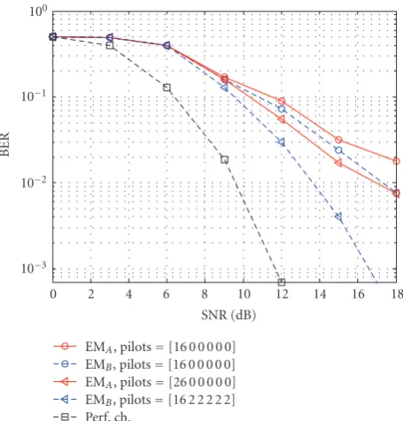
InFigure 3, we compare both schemes with 16 pilots in
the initialSTblock and zero pilots in the subsequent blocks. EMA refers to the iterative MMSE scheme whileEMB refers
to the Kalman filter-based scheme proposed in this paper. We also implement both schemes with a total of 26 pilots as shown inFigure 3. TheEMAconfines the pilots to the first
STblock while inEMB, we place 16 pilots in the firstSTblock
and 2 pilots each in subsequent blocks. This ensures that both schemes incur the same pilot overhead.
Our algorithm (EMB) outperformsEMAof [17] in both
pilot scenarios. One reason for this performance improve-ment is that our algorithm incorporates the time correlation information and the most recent channel estimate inevery iteration of theEMalgorithm, while that of [17] does not.
5.1.2. Effect of number of iterations
In this section, we test the sensitivity of our algorithm to the number of EM iterations used. Here, we employ six pilots per OFDM symbol (in addition to the 16 pilots per symbol employed in the firstSTblock). FromFigure 4, we see that the first iteration yields substantial improvement over the pilot-based estimation. The enhanced performance with increased number of EM iterations is also evident from
Figure 4. This improved performance comes at the cost of
increased computational complexity.
0 2 4 6 8 10 12 14 16 18
SNR (dB) 10−3
10−2 10−1 10
BER
EMA, pilots=[16 0 0 0 0 0]
EMB, pilots=[16 0 0 0 0 0]
EMA, pilots=[26 0 0 0 0 0]
EMB, pilots=[16 2 2 2 2 2]
Perf. ch.
Figure 3: Comparison of EM-MMSE(EMA) and EM-FB-Kalman
(EMB) algorithms.
0 5 10 15
SNR (dB) 10−5
10−4 10−3 10−2 10−1 100
BER
Pilots only Iter=1
Iter=4 Perf. ch.
Figure4:BERperformance with different number ofEMiterations.
5.1.3. Effect of incorporating frequency and time
correlation in the channel estimation
The impact of using both frequency and time correlations in channel estimation is shown inFigure 5for the six-pilot scenario. In this figure,Ie = 1 (whereIe stands for
“infor-mation used in esti“infor-mation”) refers to channel esti“infor-mation using either frequency or time correlation information only while Ie = 2 implies the use of both frequency and time
0 5 10 15 20 SNR (dB)
10−4 10−3 10−2 10−1 100
BER
Pilots only,Ie=1 (time)
Iter=1,Ie=1 (time)
Pilots only,Ie=1 (frequency)
Iter=1,Ie=1 (frequency)
Pilots only,Ie=2
Iter=1,Ie=2
Perf. ch.
Figure5: Effect of a priori correlation knowledge on the
perfor-mance of the receiver.
used in channel estimation. (By using frequency correlation only, we mean a receiver that estimates the channel using least squares, i.e., by performing the minimization in (28). This could equivalently be performed by implementing the FB-Kalman (35)–(41) with the matrix F set to zero. Similarly, the time correlation only case can be performed by implementing theFB-Kalman (35)–(41) with the matrix
Gset to1−α2(p)I. It should be clear that it is not possible to ignore the frequency correlation completely but by using this setting, its effect is only decreased as the channel taps do not follow the exponential channel decay profile and become identically distributed.) This error floor remains regardless of the number of iterations. However, when we incorporate both frequency and time correlation information, we observe a significant improvement in BER. We also note that a single EMiteration provides substantial improvement when compared to the pilot-based estimation case. We conclude that including both time and frequency correlations in the channel estimation process (especially for channels with high time correlation) increases the amount of information that can be harnessed by iterating.
5.1.4. Effect of time variation
In this section, we test the performance of our receiver against different degrees of time variation. This is parameter-ized byα(0≤α≤1) with lower values ofαindicating a more time-variant channel. (According to IEEE 802.16 standards, the typical range forαis 0.677 to 0.9398 for a vehicle speed decreasing from 120 km/h to 50 km/h, resp.) In Figure 6, we show theBERcurves for a system that employs six pilots perOFDMsymbol. We observe an error floor as the channel variation increases. So, we are unable to capture the time
0 5 10 15
SNR (dB) 10−6
10−5 10−4 10−3 10−2 10−1 100
BER
Iter=1,α=0.7 Iter=1,α=0.8 Iter=1,α=0.985
Perf. ch.,α=0.985 Perf. ch.,α=0.8 Perf. ch.,α=0.7
Figure6:BERperformance with varying time correlation with six pilots.
0 2 4 6 8 10 12
SNR (dB) 10−7
10−6 10−5 10−4 10−3 10−2 10−1 100
BER
Iter=1,α=0.985 Iter=1,α=0.7 Iter=1,α=0.8 Iter=1,α=0.3
Perf. ch.,α=0.985 Perf. ch.,α=0.8 Perf. ch.,α=0.7 Perf. ch.,α=0.3
Figure7:BERperformance with varying time correlation with ten pilots.
diversity. More pilots are thus needed to capture diversity and improve performance.
0 2 4 6 8 10 12 14 SNR (dB)
10−7 10−6 10−5 10−4 10−3 10−2 10
BER
Kalman with hard data FB Kalman with hard data Kalman with soft data
FB Kalman with soft data Perf. ch.
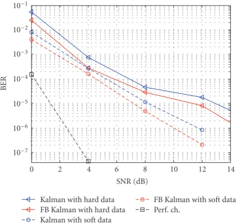
Figure8:BERperformance of Kalman andFB-Kalman using hard and soft estimate of data.
5.2. TheFBKalman
To test the FB Kalman filter, we use an input similar to the one employed in the forward-only Kalman case. The outer encoder in this case is a rate 1/2 convolutional encoder. The number of transmitters is two as Alamouti code is used in this case also and the number of receivers is also fixed at two. We use twoMIMOchannel models in this case. One is spatially white while the other one is spatially correlated with transmit and receive correlation matrices
T(p)=
1 ζ ζ 1
, R(p)=I, (59)
whereζ = 0.2. All other parameters are the same in both channel models, that is,α=0.8,β=0.2, andP=16.
Packets are transmitted at eachSNR-value until a mini-mum number of errors (five in this case) occur. Similar to the forward-only Kalman case, each packet consists of sixST blocks. The firstSTblock contains 16 pilots while the number of pilots in subsequent blocks remains fixed at 12.
Figure 8compares the Kalman and theFB-Kalman over
spatially white channel. The results are shown for two scenarios. In one, hard estimate of data (the estimated data) is used while in the other soft estimate (expected value of the data) is used. The figure clearly illustrates that theFB-Kalman is better than the Kalman for both scenarios. It can also be observed from this figure that theFB-Kalman using soft estimate of data outperforms the one using hard estimate.
The performance of Kalman and the FB-Kalman is compared in Figure 9 over the two channel models, that is, spatially correlated and spatially white channel model. In both cases, soft estimate of data is used. In the perfect channel scenario, the increased diversity in uncorrelated (white) case gives a betterBERcompared to the correlated case. However, in the estimated channel case, diversity is
0 2 4 6 8 10 12
SNR (dB) 10−7
10−6 10−5 10−4 10−3 10−2 10−1 10
BER
Kalman over spatially correlated ch. FB Kalman over spatially correlated ch. Kalman over spatially white ch. FB Kalman over spatially white ch. Perf. spatially correlated ch. Perf. spatially white ch.
Figure9:BERperformance of Kalman andFB-Kalman using soft data over spatially white and correlated channel models.
a two-edged sword. On the one hand, increased diversity should improve performance if we manage to have a good estimate of the channel. On the other hand, increased diversity also increases the channel’s degrees of freedom giving an inferior estimate to the uncorrelated case for the same number of pilots used. This explains why in the estimated case, the correlated channel performs better than the uncorrelated channel for the channel estimate quality in the former is better than the channel quality in the latter.
6. CONCLUSION
In this paper, we have proposed a receiver for MIMO-OFDM transmission over time-variant channels. While the paper assumed the channel to be constant within any ST block, the channel was allowed to vary from one block to the next. This makes the receiver suitable for operation in high-speed environments.
correlation in (A.16), and space-time coding. It is also straightforward to incorporate the effect of an outer code, sparsity, and the cyclic prefix (see [27,36]). Our simulations show the favorable behavior of the two Kalman filters as compared to other receivers.
APPENDICES
A. CHANNEL MODEL IN THE PRESENCE OF SPATIAL CORRELATION
In what follows, we derive the dynamical model for the channel impulse response in the transmit correlation case, and then generalize our results ofSection 2.2 to deal with the general (transmit and receive) correlation case. In the transmit correlation case, H(p), theMIMOimpulse response at tapp, is given by
H(p)=W(p)T1/2(p), (A.1)
whereT1/2(p) is the transmit correlation matrix (of sizeT
x)
at tappand whereW(p) consists of iid elements. The matrix
W(p) remains constant over a single STblock and varies from oneSTblock to the next according to
Wt+1(p)=α(p)Wt(p) +1−α2(p)
e−βpU
t(p), (A.2)
where α(p),β, and Ut(p) are as defined in Section 2.2.
(We suppress the time dependence at times for notational convenience.)
Just as we did inSection 2.2, we would like to construct a recursion for the tap htx
rx(p) and subsequently scale it up
for theSISOandMIMOcases. Now sincehtx
rx(p) is the (rx,tx)
element ofH(p), we deduce from (A.1) that it is the inner product of therxrow ofW(p) and thetxcolumn ofT1/2, that
is,
htx
rx(p)=wrx(p)t
tx(p). (A.3)
Moreover, from (A.2), we have the following recursion for
wrx(p):
wrx,t+1(p)=α(p)wrx,t(p) +
1−α2(p)e−βpu rx,t(p).
(A.4)
Postmultiplying both sides byttx(p) yields
wrx,t+1(p)t
tx(p)=α(p)w
rx,t(p)t
tx(p)
+1−α2(p)e−βpu rx,t(p)t
tx(p).
(A.5)
This means thathtx
rx(p) satisfies the dynamical equation
htx
rx,t+1(p)=α(p)h
tx
rx,t(p) +
1−α2(p)e−βputtx
rx,t(p),
(A.6)
whereuttx
rxis defined by
uttx
rx(p)=urx(p)t
tx(p). (A.7)
Concatenating (A.6) for p = 1, 2,. . .,P yields a dynamic equation for the impulse response
htx
rx=
⎡ ⎢ ⎢ ⎢ ⎣
htx
rx(0)
.. .
htx
rx(P)
⎤ ⎥ ⎥ ⎥ ⎦= ⎡ ⎢ ⎢ ⎢ ⎣
wrx(0)t
tx(0)
.. .
wrx(P)ttx(P)
⎤ ⎥ ⎥ ⎥
⎦, (A.8)
which is the same as the dynamic equation (see (5)) for the spatially uncorrelated case
htx
rx,t+1=Fh
tx
rx,t+Gut
tx
rx,t. (A.9)
The only difference from the uncorrelated case is thatuttx
rxis
no more white. Rather, we have
Euttx
rxut
tx∗
rx Δ =E ⎡ ⎢ ⎢ ⎢ ⎢ ⎢ ⎣
urx(0)t
tx(0)
urx(1)t
tx(1)
.. .
urx(P)t
tx(P)
⎤ ⎥ ⎥ ⎥ ⎥ ⎥ ⎦
×ttx∗(0)u∗
rx(0) t
tx∗(1)u∗
rx(1) · · · t
tx∗(P)u∗
rx(P)
= ⎡ ⎢ ⎢ ⎢ ⎢ ⎢ ⎣
tttx
tx(0)
tttx
tx(1)
. ..
tttx
tx(P)
⎤ ⎥ ⎥ ⎥ ⎥ ⎥ ⎦ Δ
=diagtttx
tx
,
(A.10)
where
tttx
rx=
⎡ ⎢ ⎢ ⎢ ⎢ ⎣
trx∗(0)ttx(0)
trx∗(1)ttx(1)
.. .
trx∗(P)ttx(P)
⎤ ⎥ ⎥ ⎥ ⎥ ⎦= ⎡ ⎢ ⎢ ⎢ ⎢ ⎣
trx(0)ttx(0)
trx(1)t
tx(1)
.. .
trx(P)ttx(P)
⎤ ⎥ ⎥ ⎥ ⎥
⎦, (A.11)
and where the second line follows from the fact thattrx∗(p)=
ttx(p) sinceT1/2(p) is conjugate symmetric. In general, we
can show that
Eutrxut∗rx
= ⎡ ⎢ ⎢ ⎢ ⎢ ⎢ ⎣
diagtt11
diagtt21
· · · diagttTx
1
diagtt1 2
diagtt2 2
· · · diagttTx
2
..
. ... · · · ... diagtt1
Tx
diagtt2
Tx
· · · diagttTx
Tx ⎤ ⎥ ⎥ ⎥ ⎥ ⎥ ⎦, (A.12)
forrx=rxand is zero otherwise. Alternatively, we can write
this as
Eutrxut∗rx
= ⎧ ⎪ ⎪ ⎪ ⎪ ⎨ ⎪ ⎪ ⎪ ⎪ ⎩ P
p=0
T(p)⊗IpBIp forrx=rx,
O otherwise,
where
B =
⎡ ⎢ ⎢ ⎢ ⎢ ⎣
1 0 · · · 0 0 0 · · · 0
..
. ... · · · ... 0 0 · · · 0
⎤ ⎥ ⎥ ⎥ ⎥ ⎦,
I =
⎡ ⎢ ⎢ ⎢ ⎢ ⎢ ⎢ ⎢ ⎢ ⎣
0 1 0
1 . .. . .. 0
1 0
⎤ ⎥ ⎥ ⎥ ⎥ ⎥ ⎥ ⎥ ⎥ ⎦
,
I =
⎡ ⎢ ⎢ ⎢ ⎢ ⎢ ⎢ ⎢ ⎢ ⎣
0 1
0 . .. . .. 1
0 1 0
⎤ ⎥ ⎥ ⎥ ⎥ ⎥ ⎥ ⎥ ⎥ ⎦
.
(A.14)
Collecting (A.9) for all transmit and receive antennas yields
ht+1=
ITxRx⊗F
ht+
ITxRx⊗G
utt, (A.15)
where
Euu∗=IRx⊗E
utrxut
∗
rx
=
P
p=0
IRx⊗T(p)⊗
IpBIp. (A.16)
When the channel exhibits both transmit and receive corre-lations, the IRhcontinues to satisfy the dynamical equation (A.15) except that the correlation of the innovationuis now given by
Euu∗=
P
p=0
R(p)⊗T(p)⊗IpBIp. (A.17)
B. CALCULATING THE MOMENTS OFX
In this appendix, we demonstrate that the four moments (56) of the uncodedOFDMsymbolS(nu) are enough to calculate
the first two moments of X,E[X], and E[X∗X]. Since X
depends linearly on ReS(nu) and ImS(nu) (see (13) and
(16)), it is straight forward to calculate the mean ofXstarting from the means of ReS(nu) and ImS(nu).Now from (16),
we note that evaluatingE[X∗X] boils down to evaluating the cross correlation E[diag(Xi∗(nc))diag(Xj(nc))], recall also
that
Xtx
nc
=
Nu
nu=1
atx,nc
nu
ReSnu
+jbtx,nc
nu
ImSnu
.
(B.1)
This means that calculating the cross expectation boils down to calculating the cross correlation of ReS(nu), ImS(nu),
ReS(nu), and ImS(nu) for nu,nu = 1,. . .,Nu. It is easy
to see that these variables are independent for nu=/ nu.
Moreover, since the noise in (52) is white, one can also see that ReS(nu) and ImS(nu) are independent. As a
result, we can completely characterize the cross correlation E[diag(Xi∗(nc))diag(Xj(nc))] and hence the expectations
E[X] and E[X∗X] starting from the first and second moments of (56).
ACKNOWLEDGMENTS
This work was supported by King Abdul Aziz City for Science and Technology (KACST), Saudi Arabia, Project no. AR 27-98. Earlier versions of this work appeared at Signal Processing Advances for Wireless Communications Workshop (SPAWC), Helsinki, Finland, June 2007 [37] and IEEE Global Telecommunications Conference (GLOBE-COM), Texas, USA, December 2004 [38].
REFERENCES
[1] A. Paulraj, R. Nabar, and D. Gore, Introduction to Space Time Wireless Communications, Cambridge University Press, Cambridge, UK, 2003.
[2] Y. Li, N. Seshadri, and S. Ariyavisitakul, “Channel estimation for OFDM systems with transmitter diversity in mobile wireless channels,”IEEE Journal on Selected Areas in Commu-nications, vol. 17, no. 3, pp. 461–471, 1999.
[3] R. Negi and J. Cioffi, “Pilot tone selection for channel estimation in a mobile OFDM system,”IEEE Transactions on Consumer Electronics, vol. 44, no. 3, pp. 1122–1128, 1998. [4] F. Tufvesson and T. Maseng, “Pilot assisted channel estimation
for OFDM in mobile cellular systems,” inProceedings of the 47th IEEE Vehicular Technology Conference (VTC ’97), vol. 3, pp. 1639–1643, Phoenix, Ariz, USA, May 1997.
[5] S. Ohno and G. B. Giannakis, “Optimal training and redun-dant precoding for block transmissions with application to wireless OFDM,”IEEE Transactions on Communications, vol. 50, no. 12, pp. 2113–2123, 2002.
[6] Y. Li, “Pilot-symbol-aided channel estimation for OFDM in wireless systems,” in Proceedings of the 49th IEEE Annual Vehicular Technology Conference (VTC ’99), vol. 2, pp. 1131– 1135, Houston, Tex, USA, May 1999.
[7] I. Barhumi, G. Leus, and M. Moonen, “Optimal training design for MIMO OFDM systems in mobile wireless chan-nels,”IEEE Transactions on Signal Processing, vol. 51, no. 6, pp. 1615–1624, 2003.
[8] R. W. Heath Jr. and G. B. Giannakis, “Exploiting input cyclostationarity for blind channel identification in OFDM systems,”IEEE Transactions on Signal Processing, vol. 47, no. 3, pp. 848–856, 1999.
[9] B. Muquet, M. de Courville, P. Duhamel, and V. Buzenac, “A subspace based blind and semi-blind channel identification method for OFDM systems,” inProceedings of the 2nd IEEE Workshop on Signal Processing Advances in Wireless Communi-cations (SPAWC ’99), pp. 170–173, Annapolis, Md, USA, May 1999.
[10] H. B¨olcskei, R. W. Heath Jr., and A. J. Paulraj, “Blind chan-nel identification and equalization in OFDM-based multi-antenna systems,”IEEE Transactions on Signal Processing, vol. 50, no. 1, pp. 96–109, 2002.