Volume 2009, Article ID 917354,22pages doi:10.1155/2009/917354
Research Article
A Reconfigurable Architecture for Rotation Invariant Multi-View
Face Detection Based on a Novel Two-Stage Boosting Method
Jinbo Xu,
1Yong Dou,
1and Zhengbin Pang
21National Laboratory for Parallel and Distributed Processing, National University of Defense Technology, Changsha 410073, China 2Institute of Computer, School of Computer, National University of Defense Technology, Changsha 410073, China
Correspondence should be addressed to Jinbo Xu,[email protected]
Received 30 December 2008; Revised 9 May 2009; Accepted 19 August 2009
Recommended by Liang-Gee Chen
We present a reconfigurable architecture model for rotation invariant multi-view face detection based on a novel two-stage boosting method. A tree-structured detector hierarchy is designed to organize multiple detector nodes identifying pose ranges of faces. We propose a boosting algorithm for training the detector nodes. The strong classifier in each detector node is composed of multiple novelly designed two-stage weak classifiers. With a shared output space of multicomponents vector, each detector node deals with the multidimensional binary classification problems. The design of the hardware architecture which fully exploits the spatial and temporal parallelism is introduced in detail. We also study the reconfiguration of the architecture for finding an appropriate tradeoffamong the hardware implementation cost, the detection accuracy, and speed. Experiments on FPGA show that high accuracy and marvelous speed are achieved compared with previous related works. The execution time speedups range from 14.68 to 20.86 for images with size of 160×120 up to 800×600 when our FPGA design (98 MHz) is compared with software solution on PC (Pentium 4 2.8 GHz).
Copyright © 2009 Jinbo Xu et al. This is an open access article distributed under the Creative Commons Attribution License, which permits unrestricted use, distribution, and reproduction in any medium, provided the original work is properly cited.
1. Introduction
Over the years, great advances have been achieved on face detection research [1], which has already been widely applied in many real-world applications, such as biometrics, visual surveillance, human-computer interaction, to name a few. Some early works on face detection, for instance, Rowley’s
ANN method [2] and Schneiderman’s method based on
Bayesian decision rule [3], have achieved high accuracy, but their applications are very limited due to the tremendous computational load. The break through happened in 2001
when Viola and Jones [4] developed their Boosted Cascade
Framework whose remarkable performance owes to the fast speed of Haar-like feature calculation based on the integral image, the high accuracy of boosted strong classifiers, and the asymmetric decision making of the cascade structure.
Frontal face images at 384×288 resolutions were reported
to be fairly reliably detected at 15 frames per second by using PC with PIII 700 MHz CPU.
Although many early researches have good performance in detection of frontal faces, multiv-iew face detection (MVFD) remains a challenging problem that needs more
attention due to the much more complicated variation within the multi-view face class. MVFD is used to detect upright faces in images that with±90◦rotation-out-of-plane (ROP) pose changes. Rotation Invariant MVFD (RIMVFD)
means to detect faces with both ±90◦ ROP and 360◦
rotation-in-plane (RIP) pose changes. Statistics show that most of the faces in images and videos of real world are nonfrontal [5], and therefore, the ability to deal with multi-view faces is important for many face-related applications.
In the past few years, many derivatives of Viola’s work have been proposed for rotation invariant frontal face detection and MVFD. These derivatives can be categorized into four aspects: the detector structure, designing of strong classifiers, training of weak classifiers, and selecting of features. For the detector structure, Viola’s cascade detector structure is extended by Wu’s parallel cascades structure [6],
Li’s pyramid structure [7], Jones’s decision tree [8], and
Huang’s WFS (width-first-search) tree in [9]. For designing
strong classifiers, the discrete AdaBoost was replaced by real
AdaBoost [10], Gentle Boost [11], boosting chain learning
replaced by finer partition of the feature space such as piece-wise functions [6] or joint binarizations of Haar-like features [14]. As for the feature level in particular, there are works of Lienhart’s extended Haar-like feature set [15], Liu’s Kullback-Leibler Boosting [16], Baluja’s pair-wise points [17], Wang’s
RNDA algorithm [18], and Abramson’s control point [19].
Most of these works focus on increasing the detection accuracy. However, these methods are only evaluated by using software solution, which can hardly achieve real-time MVFD for some time-constraint applications. There is still much work to do from the algorithm design to the ultimate practical systems.
In order to meet the needs of various applications, using
dedicated hardware to accelerate RIMVFD is an effective
solution. Without losing detection accuracy, there are several valuable advantages with dedicated hardware solution: (1) compared with the software solution, significant speedups of execution time could be achieved by fully exploiting tempo-ral and spatial patempo-rallelism; (2) the system can be dynamically
reconfigured to meet different requirements on accuracy,
speed, and resources for various applications; (3) low power consumption and high mobility can be achieved, which is very useful for small battery driven devices and handheld devices; (4) the cost could be low for commercial perspective. In literature, there are hardware implementations of frontal
face detection based on tone color detection [20, 21],
Neural Networks [22], and AdaBoost [23]. However, few
researches focus on hardware implementation of RIMVFD.
Since different applications have different demands on the
accuracy, speed, and resources cost, it is necessary to research on the reconfigurable hardware architecture for RIMVFD.
In this paper, a fine-classified method and an FPGA-based reconfigurable architecture for RIMVFD are presented. Firstly, a tree-structured detector hierarchy for RIMVFD is designed to organize detector nodes for both RIP and ROP pose changes. To train branching nodes of the detector tree, a fine-classified boosting algorithm with a novel two-stage weak classifier design is proposed. Then, the temporal and spatial parallelism of the proposed RIMVFD method is fully exploited. Next, the reconfigurable architecture for RIMVFD is designed and implemented on FPGA. The correlation among the hardware implementation cost, the detection accuracy and speed is evaluated, so that the system can
be correctly reconfigured for different applications with
different requirements. The main contributions of this paper
are
(i) RIMVFD with all ±90◦ ROP and 360◦ RIP pose
changes is achieved by using tree-structured detector hierarchy and fine-classified boosting method;
(ii) the execution time of the classification procedure is significantly reduced by fully exploiting the paral-lelism;
(iii) by dynamically reconfiguring the hardware
architec-ture, the tradeoffamong the hardware
implementa-tion cost, the detecimplementa-tion accuracy, and speed is well tuned, so that the proposed design can easily meet the demands of different applications.
The remainder of this paper is organized as follows. In Section 2, the proposed RIMVFD method is described.
Section 3presents the hardware architecture model for the proposed RIMVFD on FPGA. The reconfigurable character-istics of architecture are analyzed inSection 4.Section 5gives the experimental results. Concluding remarks are presented inSection 6.
2. Proposed RIMVFD Method
2.1. Review of AdaBoost. The basic idea introduced by
Schapire and Freund [24–26] is that a combination of
single rules or “weak classifiers” gives a “strong classifier.” A training procedure uses a training sample set to obtain multiple weak classifiers iteratively.
We define the weighted learning setSofpsamples as
S=x1,y1,w1
,x2,y2,w2
,. . .,xp,yp,wp
. (1)
The ith sample is defined by a feature vector xi =
(c1,c2,. . .,cD)T in aD-dimensional space, its corresponding
class C(xi) = yi ∈ {−1, +1} in the binary case, and the
weight of the samplewi, wherecjinxi,i = 1, 2,. . .,p, and
j = 1, 2,. . .,D, represents theith sample’s feature value at thejth dimension.
A weak classifierhtobtains a hypothesis whether a sample
belongs to a class,ht(x), according to the feature values in
the D-dimensional space. For example, whether a sample
belongs to a subwindow in an image can be hypothesized by using the horizontal and vertical coordinates (c1,c2)T as
feature values in a 2-dimensional space. If yi=/ht(xi), the
weak classifierhtmakes a wrong decision on theith sample;
otherwise, the decision is right.
Each iteration of the process consists in finding the best possible weak classifier, that is, the classifier for which the error is minimum. After each iteration, the weights of the misclassified samples are increased, and the weights of the well-classified sample are decreased. The iterative procedure stops ifεt=0 orεt≥1/2. The reason is in [25]: in the case of
binary classification (k=2), a weak hypothesishtwith error
significantly larger than 1/2 is of equal value to one with error significantly less than 1/2 sinceht can be replaced by 1–ht;
and fork >2, a hypothesishtwith errorεt≥1/2 is useless to
the boosting algorithm. If such a weak hypothesis is returned by the weak learner, the algorithm simply halts, using only the weak hypotheses that were already computed (i.e., set the number of weak classifiers in the strong classifierT=t–1).
The final strong classifier f is given by
f(x)=sgn
⎛ ⎝T
t=1
atht(x)
⎞
⎠, (2)
where both αt and ht are to be learned by the boosting
procedure presented inAlgorithm 1.
(1) InputS= {(x1,y1,w1), (x2,y2,w2),. . ., (xp,yp,wp)}, number of iterationsT. (2) Initializew(0)i =1/ pfor alli=1,. . .,p.
(3) Do fort=1,. . .,T
(3.1) Train classifier with respect to the weighted samples set and obtain hypothesis ht: S→ {−1, +1}.
(3.2) Calculate the weighted errorεtofht: εt
p i=1w
(t)
i I(yi=/Ht(xi)). (3.3) Compute the coefficientαt:
αt=1
2log
(1−εt)
εt
.
(3.4) Update the weights
wi(t+1)= wi(t)
Zt exp{−αtyiht(xi)}, whereztis a normalization constant:
Zt=2εt(1−εt) (4) Stop ifεt=0 orεt≥1/2. SetT=t−1.
(5) Output:f(x)=sgn (Tt=1atHt(x)).
Algorithm1: The basic AdaBoost procedure.
Source image Integral
image
Feature pool Image rescaler
Feature values for
all sub-windows
Stage 1 Stage 2 StageN Classifier
Pass
Pass Pass
Fail Fail Fail
Further processing
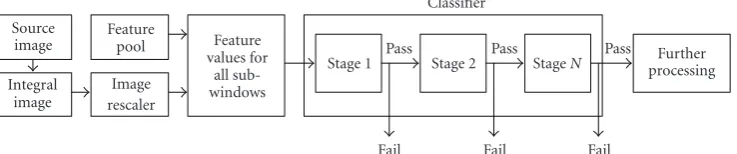
Figure1: Framework of AdaBoost-based face detection.
AdaBoost algorithm presents two significant advantages; it has the ability to quickly eliminate nonface regions, and the classification process itself is extremely fast.
While Haar wavelets were used in [27] for representing
faces and pedestrians, Viola and Jones proposed the use of
Haar-like features which can be computed efficiently with
integral image [28]. Each feature consists of a set of black
and white rectangles. The result of a feature is the sum of the pixels under the white rectangle minus the sum of the pixels under the black rectangle. In Viola’s cascade framework, a group of features composes a classification stage based on AdaBoost. The outcome of a stage determines whether the region of the image examined contains a face or not. The size of the feature determines the size of the image region being searched. When the base size is processed for all regions, the features are then enlarged in subsequent scales, and evaluated for each scale to be able to detect faces of larger sizes. Additional algorithm details can be found in [28]. The algorithm outline is shown inFigure 1.
The difference between our RIMVFD method and the
framework in Figure 1 is mainly reflected in the classifier
part. The integral image computation and image rescaler are the same, which are widely used in face detection domain currently. In this paper, we will focus on the classifying strategy of RIMVFD.
2.3. Tree-Structured Detector Hierarchy for RIMVFD. For
RIMVFD, new detector hierarchy different from the cascaded
structure for frontal face detection has to be designed,
since pose changes should be identified in addition to the
face/nonface classification. Huang et al. [9] reviewed some
traditional structures for organizing detector nodes, such as parallel cascades structure [6], pyramid structure [7],
and decision tree method [8]. After having analyzed the
weaknesses of these structures, Huang proposed a WFS-tree structure, who claimed that the structure can balance the face/nonface distinguishing and pose identification tasks, so as to enhance the detector in both accuracy and speed. Because of limited parallel processing ability in general-purpose processor, Huang’s tree structure only divides all faces into 5 categories according to ROP to control the computational cost, which is not so fine-grained.
In this paper, we extend Huang’s tree structure so as to achieve more accuracy and speed with the aid of reconfigurable hardware acceleration. The extended tree
structure covers all±90◦ ROP and 360◦RIP pose changes.
The coarse-to-fine strategy is adopted to divide the entire face space into smaller and smaller subspaces as shown in
Figure 2.
Whether a face sample belongs to a pose range or not is determined by the output of a detector node corresponding to the current pose range. The output of the detector node is a Boolean valueg(x). InFigure 2, all detector nodes which have the same parent node are trained with the same training sample set belonging to the parent pose range. The outputs
of these detector nodes form a determinative vectorG(x)=
(g1(x),. . .,gk(x)), where k is the number of the detector
360◦RIP, [−90◦, 90◦]
ROP face classifier [−45◦, 45◦]
RIP classifier
[45◦, 135◦] RIP classifier
[135◦,−135◦]
RIP classifier
[−135◦,−45◦]
RIP classifier
[−90◦,−30◦] ROP classifier
[−30◦, 30◦] ROP classifier
[30◦, 90◦] ROP classifier [−90◦,−70◦]
ROP classifier
[−70◦,−50◦]
ROP classifier
[−50◦,−30◦]
ROP classifier
[−45◦,−15◦] RIP classifier
[−15◦, 15◦] RIP classifier
[15◦, 45◦] RIP classifier
· · ·
· · · · · · · · ·
· · · · · ·
Figure2: Illustration of the proposed fine-grained tree structure.
the leaf nodes, the RIP and ROP ranges that the sample lies in are determined, from which the pose of the sample is classified.
The main extensions of the tree structure different from
the one in [9] are that the ROP and RIP granularity are
refined for more accuracy. And the number of detector nodes
as shown inFigure 2can be reduced about 75% (i.e., from
161 to 41 for this contribution) by using the reconfigurable computing techniques, which will be further described in
Section 3.1. With the aid of hardware acceleration, the detection speed is guaranteed.
2.4. Fine-Classified Boosting Method for RIMVFD. After designing the detector hierarchy, we need to research on the classification method for each detector node. Intrinsically,
the determination of vectorG(x) is the key problem. Take
the (−45◦, 45◦), RIP detector node inFigure 2as an example. A sample which passes through this node will be sent into (−90◦,−30◦), ROP, (−30◦, 30◦), ROP and (30◦, 90◦), ROP detector nodes in the subsequent level. At this moment,G(x)
is a 3-dimensional vector. For example, G(x) = (1, 0, 1)
means that the sample may lie in either (−90◦,−30◦), ROP or (30◦, 90◦), ROP pose range. This section proposes a
fine-classified boosting method to getG(x) fast and accurately.
The designing and training of the proposed method are detailed in this section.
Many derivations from the basic AdaBoost method have been proposed to be used for MVFD. Schapire and Singer presented a multiclass multilabel (MCML) version
of the Real AdaBoost [10], which assigns a set of labels for
each sample and decomposes the original problem into k
orthogonal binary ones. Huang et al. proposed the Vector
Boosting [9] in which both its weak learner and its final
output are vectors rather than scalars. In Huang’s method, Vector Boosting will deal with the decomposed binary classification problems in a unified framework by means of a shared output space of multicomponents vector. Each binary problem has its own “interested” direction in this output space that is denoted as its projection vector. For each
binary problem, a confidence value is calculated by using an extended version of the Real AdaBoost. Then the confidence vector composed of these confidence values is compared with
a threshold vectorBto obtain a Boolean output vector, where
each vector element indicates whether a sample belongs to the corresponding class. This kind of method only considers the confidence value for the current class while determining whether a sample belongs to this class, and does not consider confidence values for the other classes. The disadvantage is that the number of the candidate classes that a sample may belong is poorly constrained into an ideal extent, since a sample may be classified into one class by using the threshold in this dimension, and then classified into another class by using the threshold in that dimension. Actually, a face sample should only belong to a single pose class for face detection applications. Take the previous example in the first paragraph, for a sample which lies in (−90◦,−30◦) ROP pose range,G(x) is expected to be (1, 0, 0). However, it may be wrongly calculated as (1, 0, 1), which decreases the detection efficiency obviously.
The fine-classified boosting method proposed in this paper has the advantage of decreasing misclassified cases. For
example,G(x)=(1, 0, 1) mentioned before may be refined
to be (1, 0, 0) by using the proposed method. The novelty of the method is that each weak classifier in the detector tree is trained by using a two-stage boosting mechanism.
The training of all k detector nodes with the same parent
node uses the same training sample set. We useht = {ht(i)|
i=1,. . .,k}to denote the vector composed of thetth weak
classifiers in all these k detector nodes. The first stage of
ht(x) : h
t : χ → Rk is based on piece-wise decision
function, where x belongs to a sample space χ, and Rk
is k-dimensional real-value confidence space. The decision
function in this stage is used to obtain a k-dimensional
real-value confidence vector {ci | i = 1,. . .,k} for each
−150 −100 −50 0 50 100
cB
−150 −100 −50 0 50 100
cA
Figure3: Distribution of the samples in the 2D output space.
frontal and right face class). One Haar-like feature is used
for all k detector nodes with the same parent during each
iteration of training procedure. Thek-dimensional real-value
confidence vector{ci|i=1,. . .,k}is then used as the input
feature vector for the second stage ofht(x). The second stage
ht :Rk → {−1|+1}kis based on hyper-rectangle decision
function. It is trained to more precisely discriminate different dimensions by using the real confidence values generated in the first stage. The output is ak-dimensional Boolean vector,
where the ith element gives the determination whether a
sample belongs to the ith pose class. In this stage, each
output in thek-dimensional Boolean vector depends on allk
elements in the real-value confidence vector. In other words,
while deciding whether a sample belongs to the ith face
class, not only the probability that the sample belongs to the
ith face class but also the probability that the sample does
not belong to the other face classes should be considered. Since the full-mesh mapping strategy between the two stages
considers the correlation of different confidence values in
different dimensions, the pose class where a sample lies can
be classified more precisely. However, ht : χ → Rk and
ht :Rk → {−1|+1}kare combined to form the final weak
classifierht(x) : χ → {−1|+1}k in the current iteration,
which estimates whether a sample belongs to theith class or
not, wherei=1,. . .,k.
Take a 2-dimensional classification problem as an exam-ple. The samples in the training set either belong to face
classAor face classBor nonface. Then each sample will be
assigned a 2D confidence vector (cA,cB), wherecAindicates
the probability that the sample belongs to face class A,
and cB is similar. The distribution of the samples can be
illustrated as shown in Figure 3, where (cA, cB) is treated
as the 2D coordination of each sample. The blue dots are
samples in face classA, and the green ones are samples in
face classB, and the red ones are nonfaces. The vertical and
horizontal dashed lines inFigure 3illustrate the classification criterion based on single threshold, while the two rectangles illustrate the hyper-rectangle-based classification criterion.
Intuitively, the latter generates less misclassified samples than the former. For example, for the green dots which lie in the left rectangle and below the horizontal dashed line, they
are supposed to be classified as classBfaces. However, they
are considered as nonfaces by the single-threshold classifiers, which is misclassified. On the contrary, the hyper-rectangle-based classifiers can give the right decisions.
The weak learner is called repeatedly under the updated distribution to obtain multiple weak classifiers, which finally form a highly accurate classifier. Ak-dimensional shared out-put spaceH(x) is the linear combination of all trained weak
classifiers. Ann×kmatrixAmade up ofnk-dimensional
projection vectors is used to transform the k-dimensional
output space inton-dimensional confidence spaceF(x). Each dimension of the confidence space corresponds to a certain pose class. Finally, the output of the strong classifier is the sign ofF(x).
Take the previous example in the first paragraph, (−90◦,−30◦) ROP, (−30◦, 30◦) ROP, and (30◦, 90◦ ROP detector nodes use the same training sample set to get the classifiers, where the dimension of the shared output space,k, is 3. If we are dealing with the (−90◦,−30◦) ROP
and (30◦, 90◦) ROP classification problems, n is 2, and
n×k = 2×3 matrix A is ((1,0,0),(0,0,1)) consequently.
The projection vector (1,0,0) extracts 1st element from H(x) for (−90◦,−30◦) ROP pose classification. Similarly, the projection vector (0,0,1) extracts third element fromH(x) for (30◦, 90◦) ROP pose classification.
Algorithm 2gives the generalized description of the fine-classified boosting method. We define the sequence of train-ing set ofmsamples as S = {(x1,ν1,y1),. . ., (xm,νm,ym)},
wherexibelongs to a sample spaceχ,νibelongs to a finitek
-dimensional projection vector setΩwhich indicates a certain
pose class, and the label yi = ±1 indicates whether the
sample belongs to the pose class or not. For each sample,
the margin of a sample xi with its label yi and projection
vectorνiis defined asyi·(νi·ht(xi)). For example,yi =1
means that samplexibelongs to (−90◦,−30◦) ROP pose class
which is defined byvi = (1, 0, 0), while the classifierht(xi)
gives an opposite result:−1, which means that the classifier
does not consider the sample belongs to (−90◦,−30◦) ROP pose class. Therefore, the classifier makes a wrong estimation. At the moment, yi·(νi·ht(xi)) = −1. Otherwise, while
the classifier makes a right decision, yi ·(νi · ht(xi)) =
1.yi·(νi·ht(xi)) is used to update the sample weights. With
the introduction ofvi, the orthogonal component of a weak
classifier’s output makes no contribution to the updating of the sample’s weight. Consequently, it increases the weights of samples that have been wrongly classified according to the projection vector (in its “interested” direction) and decreases those with correct predictions.
Next, the training procedure of the two-stage weak classifier is described in detail.
For a classification problem that hasnclasses, given: (1) Projection vector setΩ= {ω1,. . .,ωn},ωi∈Rk
(2) Sample setS= {(x1,ν,y1),. . ., (xm,νm,ym)}, wherex∈χ,ν∈Ω,y= ±1 (I) Initialize the sample distributionD1(i)=1/mfor alli=1,. . .,m. (II) Fort=1,. . .,T
(i) Under current distribution, train the first stage of a weak classifier
ht:χ → Rk
(ii) Under current distribution, train the second stage of a weak classifier
ht :Rk → {−1|+1}k (iii) Combinehtandh
t with a full-mesh mapping strategy to form the weak classifier in the current iteration:
ht(x) :χ → {−1|+1}k (vi) Calculate the weighted errorεtofht(x)
εt=m
i=1Dt(i)·I(yi=/νi·ht(xi)) (v) Compute the coefficientαt:
αt= 1 2log
(1−εt)
εt
(vi) Update the sample distribution
Dt+1(i)=Dt(i)·exp(−αtZt·yi·(νi·ht(xi))),
whereZtthe normalization factor so as to keepDi+1as a probability distribution. (III) Stop ifεt=0 orεt≥1/2, SetT=t-1.
(IV) The final output space is
H(x)=T
t=1αtht(x).
(V) The confidence space isF(x)=AH(x), where the transformation matrixA= {ω1,. . .,ωn}T. (VI) The final strong classifier isG(x)=sgn(F(x)).
Algorithm2: A Generalized description of the fine-classified boosting method.
2.5.1. The First Stage of Weak Classifier. The first stage of weak classifier is used to get different real confidence values
forkdimensions based on the sample’s Haar-like feature. For
theith dimension, if a sample’s Haar-like feature is in a range
Ri, the sample is considered belonging to this class and a
higher confidence value is assigned to the sample; otherwise,
if a sample’s feature is in another range Ri, the sample is
considered not belonging to this class and a lower confidence value is assigned. In this way, each sample is assigned a confidence vector{ci|i=1,. . .,k}.
The classifier is based on piece-wise function, which
is more efficient than threshold-type function and can be
efficiently implemented with lookup table (LUT) [9]. It
divides the feature space into many bins with equal width and outputs a constant real value for each bin.
The objective of weak learner is to minimize the normalization factor of current round if adopting greedy strategy. Following Viola’s exhaustive search method in [4],
we enumerate a finite redundant Haar-like feature setP =
{fk(x;θk)}, 1 ≤k ≤n, and optimize a piece-wise function
for each feature so as to obtain the most discriminating one. Finally, for all detector nodes in the detector tree, 3820 Haar-like features are selected from about 48 700 features
through the training procedure as shown inAlgorithm 3. The
problem is how to get the optimal piece-wise functionμ. A
piece-wise function is configured by two parts: one is the division of feature space, the other is the constant for each division (i.e., bin). For simplification, the first one is fixed for each feature empirically, and the output constant for each bin
can be optimized as inAlgorithm 3.
When a sample passes through the first stageht : χ →
Rk, a confidence vector is obtained. Each real-value element
in the vector indicates the probability whether the sample belongs to the corresponding class. Then these confidence vectors for all training samples are sent into the second stage of weak classifier to finely discriminate different classes.
2.5.2. The Second Stage of Weak Classifier. The second stage ht :Rk → {−1|+ 1}kis used to further determine whether
a sample belongs to the ith class based on the real-value
confidence vector indicating the probability that the sample
belongs to each class. For a sample x, if its confidence
vector is{ci | i = 1,. . .,k}, it means that the probability
that the sample belongs to the ith class isci. Some related
works consider the sample belonging to any class where the confidence value is above a single threshold. Usually, this causes the sample being classified into multiple classes, which will obviously decrease the accuracy and increase the computational cost. To narrow the candidate classes, our second stage of weak classifier will learn the distribution of these confidence vectors for all samples, and generate a precise criterion to discriminate different classes. The clear
boundary among different classes can filter out most classes
that the sample does not belong actually.
Given: Sample setS= {(x1,v1,y1),. . ., (xm,vm,ym)},finite feature setP= {fk(x;θk)},1≤k≤n, and the current distributionDt(i).
(I) fork=1,. . . .n(each feature)
(i) Group all samples into different bins
Sj= {(xi,νi,yi)|xi∈binj}, binj=[(j−1)/ p,j/ p], 1≤j≤p (ii) Forj=1,. . .,p(each bin)
Using Newton-step method to compute
c∗j =arg min cj
(sjDt(i) exp(−y(νi·cj)))
(iii) Create weak classifierh(x;θk,μk) based on{c∗j}
h(x;θk,μk)=p j=1c∗jB
j P(θk), whereBP(u)j =
⎧ ⎨ ⎩
1 u /∈[((j−1)/ p,j/ p)
0 u /∈[((j−1)/ p,j/ p) j=1,. . .,p. and use equation
Zt=j
SjD+t(i) exp(−y(νi·cj))
to calculate its corresponding normalization factorZt. (II) Return the optimal weak classifier
ht(x)=arg min ht(x)
(Zt)
Algorithm3: Training of the first stage of weak classifier with piece-wise function.
implemented in parallel. Each sample has a confidence vector {ci | i = 1,. . .,k} in a k-dimensional space, and the
goal is to output a Boolean-value for each dimension to determine whether the sample belongs to the corresponding class. We define the generalized hyper-rectangle as a setHof 2kthresholds and a classyH, withyH∈ {−1, +1}:
H=θl
1,θ1u,θ2l,θu2,. . .,θlk,θuk,yH
, (3)
whereθli andθiuare the lower and upper limits of a given
interval in theith dimension. The decision function is
hH(x)=yH⇐⇒ k
i=1
ci> θil
andci< θiu
,
hH(x)= −yH, otherwise.
(4)
The core of the training of the second stage is the
hyper-rectangle setSH determination from a set of samplesS. We
use the method proposed in [30] to train the weak classifier.
The basic idea is to build around each sample {xi,yi} ∈
S a box or hyper-rectangle H(xi) containing no sample of
opposite classes, where xi is the confidence vectors of all
samples in this paper andyi= ±1. Additional details of the
training procedure can be found in [30].
3. Design of the Hardware Architecture Model
After having designed the detector hierarchy for RIMVFD, the strong classifier for each detector node and the weak classifier in each strong classifier, we will present the hardware architecture model for RIMVFD. The temporal and spatial parallelism of the proposed RIMVFD method is fully exploited on different design levels from the global structure to the weak classifiers.
3.1. Design of the Global Structure. As illustrated inFigure 1, the key parts of a face detection system based on Haar-like feature and AdaBoost are the classifier, the integral image computation and image rescaler. Although the work
in[28] suggested that rescaling a frame is more expensive
than rescaling the features, this is not always so. For an embedded system without a large cache, the loss of data locality incurred by the larger rescaled features is worse than the cost of including a small rescaling block, because loss of locality implies the main memory will be accessed for each use of integral image data, which is beyond the bandwidth
affordable in a low-cost device. We compare the bandwidth
requirements for main memory between the two rescaling methods here. For the method of re-scaling images, the sizes of feature subwindows for different rescaling levels are the same. While linearly transferring image data from main memory to onchip memory for caching, the cached data can be reused for adjacent subwindows if the subwindow is small enough. In this way, each pixel in the integral images in all rescaled levels is transferred only once, and the bandwidth requirement for processing a frame is proportional to the sum of size of integral images in all rescaled levels. Assuming
that the scaling factor is r, the data size of the original
integral image isC, and the number of re-scaled levels isl,
the bandwidth requirements can be denoted asBWimage =
C(1 + (1/r2) + (1/r2)2 +· · ·+ (1/r2)l-1). For the method
Reading frame data
Computing integral image
Level 1, class 1 classification
Level 1, class 2 classification
Level 1, classn1 classification Level 2, class 1
classification
Level 2, class 2 classification
Level 2, classn2 classification
LevelN, class 1 classification
LevelN, class 2 classification
LevelN, classnN classification Rescaling
image Phase 1
Phase 2
Phase 3
Classification procedure · · · · · ·
. . .
. . . .
. . .
. .
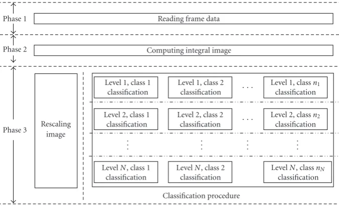
Figure4: Skeleton of the system pipeline structure.
integral image will have to be transferred more than once from main memory to onchip memory. In this situation,
the bandwidth requirements can be denoted asBWfeature =
C(a1 + a2 + · · · + al), where ai ≥ 1, i = 1, 2,. . .,l,
and ai means that some pixels in the integral image are
transferred more than once. Obviously,BWfeature> BWimage,
which means that for a system without large caches, the bandwidth requirements while rescaling features are larger than the bandwidth requirements while rescaling images. Therefore, in our work, we rescale the image instead of the features, which means that each iteration of rescaling has a corresponding rescaled integral image.
We consider the parallelism first. The phase of acquiring frames (Phase 1), computing integral frames (Phase 2), and detecting faces within frames (Phase 3) can form a pipeline, which works in a data-driven mechanism. A processing module starts operation once the needed data is available. The results will wake up the modules that are waiting for
them. As shown in Figure 4, while Phase 3 is processing
the ith frame, Phase 2 can start processing the (i+ 1)th
frame, and Phase 1 can operate on the (i + 2)th frame
simultaneously. At Phase 3, for a new frame, the input
data for image rescaler and classification procedure are both generated fromPhase 2, therefore, the image rescaler and the classification procedure can work in parallel, as illustrated in
Figure 4. Each frame is required to be rescaled to multiple scales and be processed by the classification procedure at
each scale. Therefore, at Phase 3, when the classification
procedure is processing subwindows at the jth image scale,
the image rescaler can generate rescaled integral image data
at the (j + 1)th scale. After rescaled integral image at
the (j + 1)th scale is generated, the data are sent to the
classification procedure for processing. Simultaneously, the image rescaler starts generating the (j+ 2)th rescaled integral image. During the classification procedure at each scale, the feature calculation and different classification levels in
the detector hierarchy work on different subwindows in a
Video capturer/database
Image buffer Integral image
computer
Memory interface
Main memory Display/database
Feature calculator Face classifier Detector node Face detector
module
Image rescaler
Figure5: Global architecture of the RIMVFD system.
pipelined fashion, and classifiers for different classes in the same classification level work in parallel (as shown in the
bottom right part of Figure 4). Figure 4 gives the skeleton
of the system pipeline structure. Generally, for the tree-structured detector hierarchy in this paper, the numbers of classifiers in different levels are different. The lower the level is, the more the classifiers are. Consequently,nN > · · · >
n2> n1inFigure 4.
According to the parallel characteristics of the system, the global architecture for RIMVFD is designed as illustrated in
The Face Detector module uses the tree structure illustrated in Figure 2. In each node, a Feature Calculator and a Face Classifier are included. For a new image, the Face Detector module first retrieves integral image data from the Integral Image Computer module. The classification results which indicate the position, size, and pose of each detected faces are sent back into the Main Memory for display or other purposes. After the image in the original size is processed by the Face Detector module, the rescaled integral image data are read from the Main Memory and sent into the Face Detector module for detection of faces in the current scale. As long as there are rescaled integral image data in the Main Memory which are generated by the Image Rescaler module, the procedure continues until all scales are processed for this image. Then the system starts processing another image.
It can be seen that for an image, data that should be stored in the Main Memory include the integral image data from the Integral Image Computer module, the rescaled integral image data from the Image Rescaler module and the classification results from the Face Detector module. Also data that should be read from the Main Memory include the integral image data required by the Face Detector module and the classification results required by the Dis-play/Database module. Assuming that the original image size isx×y, and the depth of the integral image pixel isdBytes, and the scaling factor isr (r >1), and the frame rate isf, and the classification results of an image occupiesRBytes, we can estimate the bandwidth requirements of the Main Memory as follows:
BW=2×f ×
x×y×d×
1 +
1 r2
2
+· · ·
+R
Bytes.
(5)
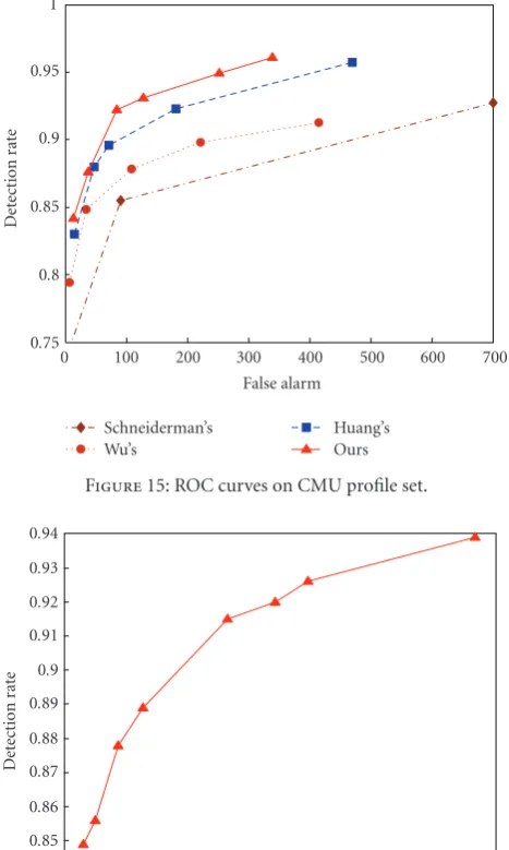
The experimental results on the bandwidth requirements are shown inTable 5.
For the computation of integral image and the rescaling
of image, the hardware structures have no much differences
with those in the frontal face detection system, which have
been researched in many related works (e.g., [23, 31]).
Therefore, we will not discuss them in this paper and focus on the design of the Face Detector Module.
The number of detector nodes as shown in Figure 2
can be reduced about 75% without significantly affecting
the speed. Since any detector node in the (45◦, 135◦),
(135◦,−135◦), and (−135◦,−45◦) RIP ranges can be gen-erated by rotating the corresponding detector node in the (−45◦, 45◦) RIP range for 90◦, 180◦, and 270◦, the detector trees for (−45◦, 45◦), (45◦, 135◦), (135◦,−135◦), and
(−135◦,−45◦) RIP ranges can reuse the same structure.
The only differences among them are the data acquisition
addresses during the feature calculation procedure. There-fore, only the (−45◦, 45◦) RIP classifier and its child nodes are configured into the FPGA chip at first, together with the root node (i.e., 360◦RIP, (−90◦, 90◦) ROP face classifier). If a subwindow is rejected by the root node, it is considered as non-face; otherwise, it flows into the (−45◦, 45◦) RIP classifier. If it is approved, it is considered as an upright face ((−45◦, 45◦) RIP) and will be further processed by the
child nodes of (−45◦, 45◦) RIP classifier until the final results are generated; otherwise, if it is rejected, the location of
the subwindow is buffered for later processing. After all
subwindows in the image are processed by the detector tree, the data acquisition scheme in the feature calculation part is updated to rotate the feature values for 90◦, 180◦, and 270◦. In this way, the (−45◦, 45◦) RIP detector tree turns into the detector trees for (45◦, 135◦), (135◦,−135◦), and (−135◦,−45◦) RIP ranges, respectively. The buffered subwindows which are rejected by the (−45◦, 45◦) RIP clas-sifier are reprocessed by the new (45◦, 135◦), (135◦,−135◦), and (−135◦,−45◦) RIP detector tree successively. Only the subwindows rejected by the 90◦RIP classifier in the previous detector tree are sent into the successive one. Since most multi-view faces concentrate in (−45◦, 45◦) RIP range in real world, the number of subwindows that are rejected by the (−45◦, 45◦) RIP classifier and need to be reprocessed by the (45◦, 135◦), (135◦,−135◦), and (−135◦,−45◦) RIP detector trees will be tiny. Consequently, although the number of
detector nodes as shown inFigure 2is reduced from 161 to
41, the detection speed is hardly affected and the detection
accuracy remains unchanged.
3.2. Organization of the Detector Hierarchy. In this section, we focus on the organization of the tree-structured detector
hierarchy. As mentioned in Figure 4, different levels work
on all subwindows in a pipelined fashion, which means that when detector nodes in the second level start processing the
jth subwindow, the nodes in the first level can work on the
(j+ 1)th subwindow. Also, classifiers for different classes in a single level work in parallel.
Different detector nodes have similar structure with
different classification parameters. The input materials of
each detector node are some feature values of sub-windows, and an enable signal indicating whether the node needs to be activated. The output of each detector node is a Boolean value indicating whether the subwindow belongs to the cur-rent face class. If the node is not a leaf node, the output will be sent into all its child nodes in the next level as their enable signals; otherwise, the output will be the final results of the detector hierarchy. In each node, cascaded structure [4] (see
Figure 1) is also adopted to organize strong classifiers in it. The motivation behind the cascade of classifier is that simple classifiers at early stage can filter out most negative subwin-dows efficiently, avoiding activating classifiers at later stages. InFigure 6, we pick up several detector nodes from two adjacent levels to explain the structure and their communi-cations. All direct child nodes of a parent node (we call them “brother nodes”) uses the same feature set. The reason is that they share the same selected features while training the first stage of weak classifiers (seeAlgorithm 3). Therefore, the feature values calculated by the Feature Calculator are sent into all direct nodes of the same parent node simultaneously.
When a subwindow passes into the parent level inFigure 6,
if the Enable Signal from the parent node of the parent level is negative, the node in the parent level will not be activated, since the subwindow is not considered to belong to this corresponding class; otherwise, the sub-window is
Stage 1 Stage 2
StageN
Stage 1 Stage 2
StageN
Stage 1 Stage 2
StageN Stage 1
Stage 2
StageN
F
eatur
e
calculat
o
r
F
eatur
e
calculat
o
r
Parent level Child level
Enable signal Feature value
· · ·
· · ·
· · ·
Figure6: Structure of detector nodes and their communications.
theStage 1is negative, the subwindow does not have to be processed by later stages in the node, which can decrease the computational cost; otherwise, the Enable Signal of the next stage will be positive. The final output of the current node is positive only if the final stage’s output is positive. The output of the parent node is connected with the Enable Signals of its direct child nodes. The workflow of these child nodes are the same with that of the parent node. We have mentioned that
different levels work on all sub-windows in a pipelined
fash-ion. Actually, different stages in a level form a pipeline as well.
3.3. Parallel Implementation of the Strong Classifier. This section will describe the structure of the strong classifiers in each cascade stage of each detector node. The design of the
strong classifier has been proposed inSection 2.4. For each
level in each direct child node of a parent detector node, the strong decision function is a particular sum of products,
where each product is made of a constantαt and the value
−1 or +1 depending on the output ofht.
Different strong classifiers have similar structure with
different classification parameters and different number of
weak classifiers. For strong classifiers in different stages of a detector node, the number of weak classifiers is different.
In addition, the constant valuesαt and the feature set used
by weak classifiers are different too. However, the constant
valuesαtand the feature set are the same for the same cascade
stage of different direct nodes of a parent node according to
the training procedure inAlgorithm 2.
We illustrate a possible structure of the strong classifier in Figure 7. However, T feature values calculated by the
Feature Calculator are sent into T weak classifiersht. Due
to the binary nature of the output of ht, it is possible to
avoid computation of multiplications. We can simply use
the output of ht to determine the sign of αt through a
multiplexer. The results ofT multiplexers are summed by a
hierarchy of adders. We can see thatT-1 addition operations
are required and the latency will be T-1 for a sequential
pipeline and log2Tfor a tree-structured pipeline, which will
slow down the processing speed whenTis large.
We can improve the above structure by decreasing the addition operations in the hierarchy of adders. The idea is that the multiplexers can be replaced by lookup table
units, and the results of additions and subtractions of αt
are encoded into them beforehand. The outputs of the weak classifiers are used as addresses of LUT units. The more additions and subtractions are encoded in a single LUT unit, the less online addition operations are required in the hierarchy of adders. The improved structure of the strong classifier with 16-bit LUT unit is presented inFigure 8.
3.4. Design of the Weak Decision Function. In this section, we will introduce the hardware structures of the two-stage weak classifiers. The design of the weak classifiers has been discussed inSection 2.5. The first stageht : χ → Rkhas the
following formula:h(x;θk,μk)=
p j=1c∗jB
j
p(θk), where
Bpj(u)=
⎧ ⎪ ⎪ ⎪ ⎪ ⎨ ⎪ ⎪ ⎪ ⎪ ⎩
1 u∈ j−1
p ,
j p
0 u /∈ j−1
p ,
j p
, j=1,. . .,p, (6)
(seeAlgorithm 3) andc∗j is trained offline. The second stage
ht : Rk → {−1|+1}k has the form of (4) for each
dimension of thekclasses.
The first and the second stages are combined to form the weak classifierht required by the strong classifier as shown
in Figure 8. For the tth weak classifier, the feature value is
sent into all dimensions of ht first, where each dimension
corresponds to each direct child node of a parent detector node. Following the decision procedure based on piece-wise
Feature calculator Sub-window
data
To stagei in other brother nodes
Hierarchy of adders sgn
MUX MUX
Stagei
h0 hT
+α0 −α0 · · · · · ·
+αT −αT
Figure7: A possible structure of the strong classifier.
Feature calculator Sub-window
data
To stagei in other brother nodes
Hierarchy of adders sgn
Stagei h0 h1 h2 h3 h4 h5 h6 h7
+α0+α1+α2+α3 +α0+α1+α2−α3 +α0+α1−α2+α3
· · · −α0−α1−α2−α3
+α0+α1+α2+α3 +α0+α1+α2−α3 +α0+α1−α2+α3
· · · −α0−α1−α2−α3
Figure8: Improved structure of the strong classifier.
of ht for further hyper-rectangle-based decision. Figure 9
shows the dataflow.
Different ht have similar structure. According to the
training procedure in Algorithm 3, the division of feature
space and the feature value as input is the same for different dimensions ofht, but the constantcare different, which will
eventually affect the outputs of different dimensions. The
derivation of the confidence values,c1,c2,. . .,cp, is based on
the training procedure inAlgorithm 3. For allkdimensions
of a set of first-stage weak classifiers ht = {h
t(i) | i =
1,. . .,k}(as shown inFigure 9), the determination of their confidence values uses the same set of training samples.
Therefore, the jth confidence value for allkdimensions can
form a confidence vector cj. Also,cj is updated iteratively
by using a proper optimization algorithm such as Newton-step method, until the training lossSjDt(i) exp(−yi(νi·cj))
is minimized. The final cj, denoted as c∗j, is then used to
construct the piece-wise decision functionht. The piece-wise
decision function can be easily implemented on hardware by
using LUT units, as shown inFigure 10(a). Each element in
an LUT unit corresponds to the constant value for a feature bin. The input is the normalized feature value, which will be used as the address for LUT. If the feature value is located
Feature calculator Sub-window
data
Featuret
Nodek Node 2
Node 1
ht(1) ht(2) ht(k)
ht(1) ht(2) ht(k) · · · · · ·
· · · · · · · · · · · · · · · · · ·
· · ·
Figure9: Dataflow of the weak decision function.
c1 c2 c2 c3 · · ·
cp Normalized
feature value
Confidence value LUT
(a) c1> θ0l
c1< θu 0
ck> θl k ck< θlk
And . . . And
And XNO
R Result c1
ck
yH
(b)
Figure10: Structures of the two-stage weak classifiers. (a) the first stage; (b) the second stage.
at the jth bin of all pbins,cjin the LUT will be selected as
output.
Differentht have similar structure, too. The confidence
values as input are the same for different dimensions of
ht. However, the classification parameters as shown in (3)
are different. The hyper-rectangle-based decision function
can be easily implemented on hardware by only using some comparison units and logical operation units, as illustrated inFigure 10(b).
4. Reconfiguration of the Architecture Model
In this section, we focus on finding automatically an
appro-priate tradeoffamong the hardware implementation cost, the
detection accuracy, and speed by dynamically reconfiguring the hardware architecture model, so that the proposed design
can easily meet the demands of different applications. The
design automation strategies are analyzed on different design levels from the global structure to the weak classifiers.
the accuracy. Therefore, we can find a tradeoffbetween the speed and accuracy by changing the scaling factor and the scanning step.
By rescaling the integral image, a pyramid framework will be generated. The calculation of pyramid poses heavy computation load. For example, given an input image
resolution of x-by-y, and the size of the sub-window for
classificationx0-by-y0, let the scaling factor ber and letSx
andSy be the steps in thex- and y-direction, respectively.
The total number of subwindows,n, can be calculated as
n≤ xy SxSy
r2−minx2
0/x2,y02/ y2
r2−1 . (7)
Typical values ofx0 and y0 is 24, and the values ofSx and
Sy are in the range of 1 to 5 pixels. When r = 1.2 and
input image size is 256×256, according to (7), nis more
than 100 000 images.
The execution time of a single frame depends directly on
the number of subwindowsn. Therefore, when the system
requires that the classification should be processed in a very high speed and the accuracy requirement is not that critical, we can achieve this by increasingr,Sxand/orSy. Otherwise,
we can decrease them.
LetlT1,lT2, andlT3denote the computation latency for a
single subwindow for Task 1 (integral image computation), Task 2 (classifier), and Task 3 (image rescaler). According to
the pipeline scheme inFigure 4, the latency for generating
a final result of a subwindow would approximately depend on the largest value amonglT1,lT2, andlT3. Therefore, the
total timeTFto process a single frame (withnsubwindows)
is approximately given by
TF=n·max(lT1,lT2,lT3). (8)
LetcT1,cT2, andcT3denote the hardware implementation
costs of Task 1, Task 2, and Task 3, respectively. Then the total cost for the key part of the system is approximately the sum of them:
ctotal=cT1+cT2+cT3. (9)
4.2. Reconfiguration on the Detector Hierarchy Level. In the detector hierarchy level, we analyze two aspects of reconfigu-ration problems. Firstly, the detection granularity and range of detector nodes in the tree-structured detector hierarchy can be reconfigured. Secondly, the number of cascaded strong classifiers can be reconfigured in each detector node.
4.2.1. Reconfiguration of the Detection Granularity and Range.
According to Section 2.3, the proposed tree structure can
cover all±90-degree ROP and 360◦RIP pose changes. The
finer the detection granularity in each pose dimension is,
the more accurate the detection is. For example, inFigure 2,
the granularity in ROP and RIP is 20◦and 30◦, respectively. Consequently, the hardware resource requirements and the power consumption will increase because of the increase of number of detector nodes. Also, the detection speed may decrease.
For different classification granularities, the detector
nodes should be retrained. The consequences are that the number of cascades in the nodes and the number of weak classifiers in the strong classifiers would be totally different. As a result, the reconfiguration of the classification granularity means that almost all detector nodes in the tree should be removed and new detector nodes are configured into the FPGA chip. The cost of this kind of reconfiguration would be a little large. Therefore, it is not so suitable for run-time reconfiguration. However, when the system is
about to be used for another purpose which has different
requirements on the detection granularity and hardware resources, the reconfiguration operation can be performed during the initialization phase. By reconfiguring the current system, there is no need to design a new system for the application.
Moreover, if the application only requires that the detection be performed in some particular ranges of pose
changes, but not all±90◦ROP and 360◦RIP pose changes,
we can achieve this by manually shut offthose absolutely
useless nodes. For example, if pose changes in the range of (−30◦, 30◦) for ROP are required to be classified, and pose changes in other ranges are not our interest and considered to be nonface directly, the corresponding detector nodes
can be manually shut off. In this way, the active nodes are
significantly reduced from 41 to 15. The cost of this kind of reconfiguration is small since only a 1-bit enable signal is required for each node and the node itself do not have to be replaced with a new one.
The hardware implementation cost of the detector
hierarchycT2can be approximately calculated as
cT2= m
i=1 ni
j=1
ci j, (10)
where ci j is the cost of the jth detector node in the ith
detector level.
4.2.2. Reconfiguration of the Cascade Number. As mentioned inSection 3.2, the cascaded structure [4] is adopted in each detector node. As discussed in [4], simple classifiers at early
stages can filter out most negative subwindows efficiently,
and stronger classifiers at later stages are only necessary to deal with instances that look like faces with some particular poses. Compared with the detector node with only one strong classifier, the power consumption will be significantly decreased since quite a few subwindows can be processed with the early simple classifiers. However, it is at the cost of hardware resources. The approximate cost of the cascaded detector node nodei j (i=1,. . .,m,j=1,. . .,ni) is
ci j= qi j
k=1
ci jk, (11)
whereci jk is the estimated hardware cost of thekth cascade
stage at the jth node in theith level.
The number of the cascades in a node can be
which demand that the power consumption be low, such as digital camera and other handheld devices, more cascades can be configured into the FPGA chip; otherwise, for applications which demand that the size and price of the device be controlled, the number of the cascades should be constrained.
4.3. Reconfiguration on the Strong Classifier Level. The num-ber of weak classifiers, denoted as Ti jk, in a single strong
classifier (we are referring to the strong classifier at the latest stage in a detector node) can also be reconfigured to
find a tradeoffbetween the detection accuracy and hardware
implementation cost. IfTi jkis smaller, the accuracy is weaker
and the hardware cost is less; otherwise, the accuracy is stronger and the cost is more.
The hardware implementation cost of a strong classifier
with Ti jk weak classifiers can be approximately estimated.
According to Figures 8 and9, a strong classifier is mainly
composed of a set of 16-bit LUT units, a hierarchy of adders and Ti jk weak classifiers containing the first stage ht, the
second stageht together with their corresponding feature
calculation units. In terms of slices, the hardware cost,ci jk,
for the strong classifier atkth cascade stage of jth detector node atith detector level, can be expressed as follows:
ci jk
=
Ti jk
t=1
ctf +cth+cth
+
Ti jk
4
·cLUT+
Ti jk
4
−1
·cadd,
(12)
where ctf,cht,cth,cLUT, andcadd are the costs of a feature
calculation unit, a first-stage weak classifierht, a second-stage
weak classifierht, a 16-bit LUT unit, and an adder, where
cLUTandcaddwill be considered as a constant.
4.4. Reconfiguration on the Weak Decision Function Level. In this section, the reconfiguration problems on the first-stage weak classifierhtand second-stageht are analyzed.
As shown inFigure 10(a), the elementary structure ofht
is an LUT unit. The number of elements in the LUT unit is the same with the division granularity of feature space. The finer the granularity is, the more accurately the function can estimate. However, more LUT elements will cost more hardware resources. Therefore, we can tune the number of
elements to meet different requirements on the accuracy and
the cost. The hardware implementation cost of the first-stage weak classifier,ch, is approximately proportional to the
number of LUT elementsu:
ch =uλ1, (13)
whereλ1is the cost for one LUT element.
As the elementary structure ofht is based on numerous
comparisons performed in parallel (see Figure 10(b)), it is
necessary to reduce the number of comparators as much as possible for minimizing the final number of used slices. If the hardware resources are limited, three particular cases
of hyper-rectangles can be considered to replace the general case as illustrated in (4) for minimizing the hardware cost.
(1) The single threshold:
T=θi,yT
, (14)
whereθi is a single threshold,i = 1,. . .,k(kis the
number of classes in the classification space), and the decision function is
hT(x)=yT ⇐⇒ci< θi,
hT(x)= −yT, otherwise.
(15)
(2) The single interval:
I=θl i,θui,yI
, (16)
where the decision function is
hI(x)=yI⇐⇒
ci> θli
andci< θiu
,
hI(x)= −yI, otherwise.
(17)
(3) The partial hyper-rectangle:
P=θl1,θ1u,θ2l,θ1u,. . .,θlp,θu1,yP
, (18)
where {θl
1,θ1u,θ2l,θ1u,. . .,θlp,θu1} are the lower and
upper limits of a randomly selected subset of the
entirek-dimensional space. And the decision
func-tion is the similar with (4):
hP(x)=yP⇐⇒ p
i=1
ci> θil
andci< θui
,
hP(x)= −yP, otherwise.
(19)
In order to optimize the final result, it is necessary to combine the previous approaches, finding for each iteration
the best weak classifier among the single thresholdhT, the
single interval hI, the partial hyper-rectangle hP, and the
general hyper-rectanglehH. The training procedure of the
second-stage weak classifierht can be optimized as shown
inAlgorithm 4.
This strategy allows minimizing the number of training iterations, and thus minimizing the final hardware cost. The hardware implementation cost of a second-stage weak
classifier,ch, is approximately proportional to the number
of comparatorsv:
ch =vλ2, (20)