From Ground Testing Facilities to Ablative Heatshields
Thesis by
Jason Rabinovitch
In Partial Fulfillment of the Requirements for the Degree of
Doctor of Philosophy
California Institute of Technology Pasadena, California
2014
Acknowledgments
First and foremost, I would like to thank my advisor, Guillaume Blanquart, for working with me over the past several years. In addition, I would like to thank my committee members, Tim Colonius, Beverley Mckeon, and Joe Shepherd, for taking the time to review my work, and for offering many insightful comments about this thesis. It has been a privilege to be surrounded by so many intelligent people throughout my entire time at Caltech.
In addition, I would like to thank all members of The FORCE and Joe Shepherd’s research group; this work would not have been possible without the help and support of all of students in these groups. In particular, I would like to thank Nick Parziale for the time we spent working together on the Vertical Expansion Tunnel and organizing the Caltech Space Challenge, for many years of softball, and for his friendship throughout my time at Caltech.
I have had the privilege of being a graduate student fellow of the Keck Institute for Space Studies since coming to Caltech. I would like to thank KISS for funding me during my first year at Caltech, and for allowing me to interact with so many leaders in the aerospace industry over the past several years. In particular, I would like to thank Michele Judd for making all of these amazing events possible, and for acting as a professional mentor to me.
The work on ablative heatshields has benefited greatly from collaborations with Vanessa Marx and R´emy Mevel. To all of my friends from home, from Yale, and from California, thank you for supporting me all of these years, and for listening to me talk about my research.
Finally, without the endless support of my parents, Marsha and Jed Rabinovitch, and my brother, Marty Rabinovitch, none of this would have been possible. Thank you.
Abstract
Motivated by recent MSL results where the ablation rate of the PICA heatshield was over-predicted, and staying true to the objectives outlined in the NASA Space Technology Roadmaps and Priorities report, this work focuses on advancing EDL technologies for future space missions.
Due to the difficulties in performing flight tests in the hypervelocity regime, a new ground testing facility called the vertical expansion tunnel is proposed. The adverse effects from secondary diaphragm rupture in an expansion tunnel may be reduced or eliminated by orienting the tunnel vertically, matching the test gas pressure and the accelerator gas pressure, and initially separating the test gas from the accelerator gas by density stratification. If some sacrifice of the reservoir conditions can be made, the VET can be utilized in hypervelocity ground testing, without the problems associated with secondary diaphragm rupture.
The performance of different constraints for the Rate-Controlled Constrained-Equilibrium (RCCE) method is investigated in the context of modeling reacting flows characteristic to ground testing fa-cilities, and re-entry conditions. The effectiveness of different constraints are isolated, and new constraints previously unmentioned in the literature are introduced. Three main benefits from the RCCE method were determined: 1) the reduction in number of equations that need to be solved to model a reacting flow; 2) the reduction in stiffness of the system of equations needed to be solved; and 3) the ability to tabulate chemical properties as a function of a constraint once, prior to running a simulation, along with the ability to use the same table for multiple simulations.
Finally, published physical properties of PICA are compiled, and the composition of the pyrolysis gases that form at high temperatures internal to a heatshield is investigated. A necessary link between the composition of the solid resin, and the composition of the pyrolysis gases created is provided. This link, combined with a detailed investigation into a reacting pyrolysis gas mixture, allows a much needed consistent, and thorough description of many of the physical phenomena occurring in a PICA heatshield, and their implications, to be presented.
Contents
Acknowledgments iii
Abstract iv
1 Introduction 1
1.1 Overview of Successful Mars Landings . . . 2
1.2 MSL—Design Considerations and Flight Data. . . 4
1.3 Organization and Objectives of Thesis . . . 5
1.3.1 Ground Testing Facilities . . . 6
1.3.2 Reacting Flows . . . 8
1.3.3 Ablative Heat Shields . . . 10
2 Vertical Expansion Tunnel 13 2.1 Motivation . . . 13
2.2 Available Conditions . . . 16
2.3 Test Time Calculation for the RST and ET . . . 19
2.4 Ideal Test Time Calculation for the VET . . . 20
2.4.1 The Compressible Euler Equations with Area Change . . . 21
2.4.2 Roe Solver . . . 23
2.4.3 Treatment of Fluid Interfaces . . . 25
2.4.4 Higher-Order Corrections . . . 26
2.4.5 Entropy Fix. . . 27
2.4.6 Numerical Results: Verification . . . 27
2.4.7 Numerical Results: VET with Nozzle . . . 29
2.5 Real Facility Effects . . . 33
2.5.2 Idealvs. Experimental Test Conditions . . . 34
2.6 Discussions . . . 36
3 Rate-Controlled Constrained-Equilibrium 38 3.1 Motivation . . . 38
3.2 Previous Work . . . 39
3.3 Reacting Euler Equations . . . 40
3.4 RCCE Overview . . . 43
3.5 Methodology for Constraint Selection . . . 47
3.5.1 Timescale Analysis . . . 47
3.5.2 Degree of Disequilibrium. . . 49
3.5.3 Effect of Elemental Conservation . . . 50
3.6 Air Test Cases—Overview . . . 51
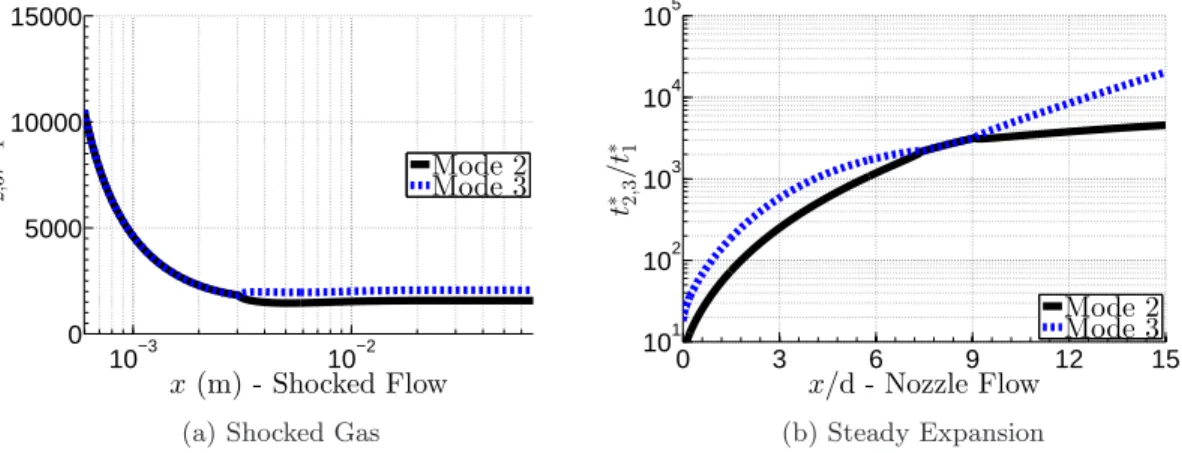
3.6.1 Case #1: Shocked Gas. . . 52
3.6.2 Case #2: Steady Expansion. . . 53
3.7 Air Test Cases—Constraint Selection . . . 54
3.7.1 Species Constraints. . . 55
3.7.2 Global Quantities. . . 55
3.7.3 Constraints based on Timescale Analysis . . . 56
3.7.4 Constraints Based on DOD Analysis . . . 59
3.8 Constraint Performance . . . 60
3.8.1 Comparison Methodology . . . 61
3.8.2 Constraint: Individual Species . . . 61
3.8.3 Constraint: Major and Radical Species. . . 68
3.8.4 Constraint: Global Quantities. . . 71
3.8.5 Constraint: Timescale Analysis andDOD . . . 75
3.8.6 Analysis of Constraint Performance . . . 78
3.9 Integrated RCCE Simulation . . . 83
3.9.1 Methodology for RCCE Simulations . . . 83
3.9.2 Tabulated Approach . . . 84
3.9.3 Integrated Simulation Results - Shock . . . 85
3.9.4 Integrated Simulation Results - Nozzle . . . 86
3.10 Extension to the Martian Atmosphere . . . 89
3.11 Discussion . . . 97
4 Pyrolysis Gas Composition in PICA Heatshields 99 4.1 Motivation . . . 99
4.2 Ablation Overview . . . 101
4.3 PICA Composition . . . 103
4.3.1 Expected Fiber Properties. . . 104
4.3.2 Expected Resin Properties. . . 105
4.3.2.1 Types and Production. . . 105
4.3.2.2 Curing and Thermal Decomposition . . . 107
4.3.2.3 Presence of Impurities . . . 108
4.3.3 Expected Char Composition. . . 109
4.4 Pyrolysis Gas Composition . . . 110
4.4.1 Equilibrium Pyrolysis Gas Composition . . . 111
4.4.1.1 Gas Model . . . 111
4.4.1.2 Elemental Composition of Pyrolysis Gases . . . 113
4.4.1.3 Equilibrium Results—PAH Species. . . 114
4.4.1.4 Equilibrium Results—Varying Mixture Composition . . . 115
4.4.1.5 Equilibrium Results—Discussion . . . 118
4.4.2 Kinetic Evolution of Pyrolysis Gas Composition . . . 119
4.5 Pyrolysis Gas Flow Regime . . . 124
4.5.1 Continuum Flow Assumption . . . 124
4.5.2 PAH Collisions . . . 126
4.5.3 PAH and Fiber Collisions . . . 128
4.6 Effect of Carbon Deposition . . . 130
4.6.1 Model #1 . . . 131
4.6.2 Model #2 . . . 132
4.6.3 Results . . . 133
4.7 Analysis of Experimental Results . . . 135
4.8 Constrained Equilibrium Calculations . . . 139
5 Conclusions and Future Work 147
5.1 Vertical Expansion Tunnel. . . 147
5.2 Rate-Controlled Constrained-Equilibrium . . . 148
5.3 Pyrolysis Gas Composition in PICA Heatshields . . . 149
Appendices 167 A Constrained Thermodynamic Equilibrium Calculations 168 B RCCE Table Sensitivity 169 C Resin Synthesis 172 C.1 General . . . 172
C.2 Curing and Decomposition Characteristics . . . 173
C.3 Synthesis of Novolac Resins . . . 174
C.3.1 Brønsted Acid Catalysts—Novolac Resins . . . 176
C.3.2 Lewis (Neutral) Acid Catalysts—High Ortho Novolac Resins . . . 176
C.4 Synthesis of Resole Resins . . . 177
C.5 Byproducts formed in synthesis of resins . . . 179
List of Figures
1.1 Three Generations of Mars Rovers . . . 4
1.2 MSL Flight Data . . . 6
1.3 Secondary Diaphragm Impacts in an Expansion Tube . . . 8
1.4 Avcoat and PICA Pyrolysis Gas Compositions . . . 11
2.1 Expansion Tunnel Schematic . . . 13
2.2 Pressure-Velocity Diagram for a Conventional Expansion Tube . . . 17
2.3 Pressure-Velocity Diagram for a Vertical Expansion Tunnel . . . 17
2.4 Schematic x-t Diagram for a Conventional ET . . . 20
2.5 Numerical Flux Correction for Fluid Interfaces . . . 25
2.6 1D Numerical x-t Diagram . . . 28
2.7 Analytic and Numerical Test Time Comparison. . . 29
2.8 Numerical x-t Diagram for an Expansion Tunnel . . . 30
2.9 x-t Diagram for Accelerator and Nozzle Sections . . . 31
2.10 Test Time Calculations for the VET . . . 32
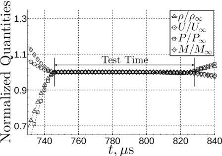
2.11 VET Normalized Flow conditions . . . 33
3.1 Overview of RCCE Method . . . 44
3.2 Species Evolution for Shocked Air . . . 53
3.3 Species Evolution for Expanding Air . . . 54
3.4 Reaction Mode Time Scales for Air . . . 57
3.5 Reaction Coefficients for Air—Fast Mode . . . 58
3.6 Degree of Disequilibrium for Air . . . 59
3.7 Shocked Air—Constraining O2 . . . 62
3.8 Shocked Air—Constraining N2 . . . 62
3.10 Shocked Air—Constraining O. . . 64
3.11 Expanding Air—Constraining O2. . . 65
3.12 Expanding Air—Constraining N2. . . 65
3.13 Expanding Air—Constraining O . . . 66
3.14 Expanding Air—Constraining NO . . . 67
3.15 Shocked Air—Constraining Major Species . . . 68
3.16 Shocked Air—Constraining Radical Species . . . 69
3.17 Expanding Air—Constraining Major Species . . . 69
3.18 Expanding Air—Constraining Radical Species . . . 70
3.19 Shocked Air—Constraining Molecular Weight. . . 71
3.20 Shocked Air—Constraining Standard Enthalpy of Formation (by Mass) . . . 72
3.21 Expanding Air—Constraining Molecular Weight . . . 74
3.22 Expanding Air—Constraining Standard Enthalpy of Formation (by Mass). . . 74
3.23 Shocked Air—Constraining Using Fast Reaction Mode . . . 75
3.24 Shocked Air—Constraint Based on DOD Analysis and Elemental Conservation . . . . 76
3.25 Expanding Air—Constraining Using Fast Reaction Mode . . . 76
3.26 Expanding Air—Constraint Based on DOD Analysis and Elemental Conservation . . 77
3.27 L2 Error Plot Air—h(To) andγ . . . 79
3.28 Weighted L2 Error Plot Air—h(To) andγ . . . 80
3.29 L2 Error Plot Air—|∂φ/∂t| . . . 80
3.30 Reconstruction ofφ—Constraining Enthalpy of Formation. . . 82
3.31 RCCE Simulation for a Shocked Gas (Mass Fractions) . . . 86
3.32 RCCE Simulation for a Shocked Gas (Constraint) . . . 87
3.33 RCCE Simulation for a Diverging Nozzle (Mass Fractions) . . . 87
3.34 RCCE Simulation for a Diverging Nozzle (Constraint) . . . 88
3.35 Species Evolution for Martian Atmosphere Processed by a Normal Shock . . . 90
3.36 Species Evolution for Martian Atmosphere Undergoing a Steady Expansion . . . 91
3.37 Shocked Mars Atmosphere—Constraining Enthalpy of Formation (by Mass). . . 92
3.38 Expanding Mars Atmosphere—Constraining Enthalpy of Formation (by Mass) . . . . 92
3.39 L2 Norm Comparisons for Mars Atmosphere . . . 93
3.40 Reconstruction ofφ(Mars Atmosphere) . . . 94
3.42 RCCE Simulation for a Shocked Flow—Mars (Constraint). . . 95
3.43 RCCE Simulation for a Diverging Nozzle—Mars (Mass Fractions) . . . 96
3.44 RCCE Simulation for a Diverging Nozzle—Mars (Constraint) . . . 96
4.1 Ablation Schematic Diagram . . . 102
4.2 PICA Material . . . 104
4.3 Idealized Resin Structure . . . 107
4.4 Equilibrium Mixture—Resin Composition . . . 114
4.5 Coronene Molecule . . . 115
4.6 Equilibrium Composition—Varying Char Yields . . . 116
4.7 Equilibrium Enthalpy Comparisons . . . 117
4.8 Maximum C24H12Mass Fraction Over a Range of Char Yields and Pressures . . . 119
4.9 Kinetic Evolution of Pyrolysis Gas . . . 121
4.10 Equilibrium Composition of Pyrolysis Gas. . . 122
4.11 Enthalpy Comparison for Equilibrium and Finite-Rate Kinetics . . . 123
4.12 Schematic for Carbon Fiber Arrangements . . . 125
4.13 Fiber/PAH Collision Schematic. . . 129
4.14 Effect of Solid Carbon Deposition (0% Char Yield). . . 134
4.15 Effect of Solid Carbon Deposition (35% Char Yield) . . . 134
4.16 Effect of Solid Carbon Deposition (60% Char Yield) . . . 135
4.17 Experimental Data Compared to Thermodynamic Equilibrium Calculations . . . 138
4.18 Comparison of Elemental Composition of Pyrolysis Gas . . . 139
4.19 Comparison of Elemental Composition of Pyrolysis Gas—Integrated . . . 140
4.20 Experimental Data Compared to Constrained Equilibrium Calculations . . . 141
4.21 Mixture Enthalpy Comparison—Sykes . . . 141
4.22 Constrained Equilibrium Composition—A1OH . . . 142
4.23 Constrained Equilibrium Composition—8 Species. . . 143
4.24 Constrained Equilibrium Composition—Summation of PAH Species . . . 144
4.25 Enthalpy Comparison for Different Constrained Equilibrium Calculations . . . 144
B.1 RCCE Results for Varying Table Resolution—Shock Mass Fractions . . . 169
B.2 RCCE Results for Varying Table Resolution—Shockφ . . . 170
B.4 RCCE Results for Varying Table Resolution—Nozzleφ . . . 171
C.1 General Synthesis of a Phenolic Resin . . . 173
C.2 Conversion of Ether to Methylene Linkages Upon Curing . . . 173
C.3 General Synthetic Scheme for the Production of a Novolac Resin . . . 175
C.4 Hexamethylenetetramine as a Source of Formaldehyde . . . 175
C.5 Brønsted Acid-Catalyzed Reaction of Phenol with Formaldehyde . . . 177
C.6 Lewis Acid Catalyzed Reaction of Phenol with Formaldehyde . . . 178
C.7 General Synthetic Scheme for the Production of a Resole Resin . . . 179
C.8 Base-Catalyzed Reaction of Phenol with Formaldehyde. . . 180
List of Tables
1.1 Summary of Successful NASA Mars Landers and Rovers. . . 3
2.1 Run Condition Comparison for RST, ET, and VET . . . 18
2.2 VET Conditions for Varying Run Conditions . . . 33
3.1 Test Case #1 Conditions . . . 52
3.2 Test Case #2 Conditions . . . 54
3.3 Summary of Constraints. . . 55
3.4 Global Constraint Examples . . . 56
3.5 Calculated Constraints Based on DOD Analysis . . . 60
3.6 Sensitivity of|∂φ/∂t| . . . 73
3.7 Sensitivity of Reaction Rates . . . 73
4.1 Summary of Phenolic Resins . . . 106
4.2 Summary of Pyrolysis Gas Compositions . . . 114
4.3 Calculated Elemental Composition of Pyrolysis Gas Reported by Sykes. . . 137
4.4 Elemental Composition of Pyrolysis Gas Reported by Tricket al. (1995) . . . 138
D.1 Species Model for Pyrolysis Gas Mixture . . . 182
Chapter 1
Introduction
The goal of this thesis is to use computational methods to advance entry, descent, and landing (EDL) technologies for future space missions. The motivation stems from a recent NASA report which identified key mission enabling technologies in order to ensure that NASA remains a world leader in technology and science.
In 2010, NASA’s Office of the Chief Technologist (OCT) drafted a set of 14 Space Technology Area Roadmaps (STARS) to identify key technologies for NASA to invest in. The Aeronautics and Space Engineering Board of the National Research Council (NRC) then appointed a steering committee to solicit external inputs and to evaluate the roadmaps. This led to the release of the report: “NASA Space Technology Roadmaps and Priorities: Restoring NASA’s Technological Edge and Paving the Way for New Era in Space” [39]. The 14 technical areas identified covered many engineering and scientific disciplines, while remaining consistent with the three overall technical objectives for NASA:
• Objective A: Extend and sustain human activities beyond low Earth orbit (LEO)
• Objective B: Explore the evolution of the solar system and the potential for life elsewhere (in situ measurements)
• Objective C: Expand our understanding of Earth and the universe in which we live (remote measurements)
This work will focus on technology development related to Technical Area 09 (TA09) “Entry, Descent, and Landing Systems”. NASA’s justification for the inclusion of EDL technologies in STARS is found in [39]:
facilitate sample returns from bodies of interest, and to enable human exploration of planets such as Mars. As the maximum mass that can be delivered to an entry interface is fixed for a given launch system and trajectory design, the mass delivered to the sur-face will require reductions in spacecraft structural mass; more efficient, lighter thermal protection systems; more efficient lighter propulsion systems; and lighter, more efficient deceleration systems.
EDL systems are mission critical technologies. The primary goal of EDL technology development is to extend the ability to deliver more payload safely to the destination. Two specific technologies needed to achieve this goal were identified to be the development of rigid thermal protection systems, and advancing EDL modeling and simulation.
Related to TA09, is TA14 “Thermal Management Systems”, where the over-arching goal is to [39]: Develop a range of rigid ablative and inflatable/flexible/deployable thermal protection systems (TPS) for both human and robotic advanced high-velocity return missions, either novel or reconstituted legacy systems.
TPS is mission-critical for all future human and robotic missions that require plane-tary entry or reentry. The current availability of high-TRL rigid ablative TPS is adequate for LEO re-entry but is inadequate for high-energy re-entries to Earth or planetary mis-sions. Ablative materials are enabling for all NASA, military, and commercial missions that require high-Mach-number re-entry, such as near-Earth asteroid visits and Mars missions, whether human or robotic.
Advancing these technologies requires a combination of theoretical, experimental, and numerical work. The report asserts that:
Adequate ground-test facilities are required to validate analytical models, to bench-mark complex computer simulations such as computational fluid dynamics models, and to examine new designs and concepts ...
Large contributions have been made to this field in the past half-century; it is important to outline some of NASA’s recent successful landings on Mars in order to understand the current state of the art in EDL technologies.
1.1
Overview of Successful Mars Landings
“Von Braun got the astronauts into space. Lester Lees got them down.” - Apollo project manager [1]
could be reached by the earth re-entry vehicle [15,30,120]. The aeroshell component of a re-entry ve-hicle is designed to both dissipate the re-entry veve-hicle’s high speeds, and to protect the payload from the extremely harsh aerothermal environment experienced during re-entry. The interaction between the vehicle’s heatshield and the atmosphere generally dissipates more than 90% of the vehicle’s ki-netic energy, which is largely converted into thermal loads that the vehicle must endure [82,94]. An accurate understanding of the aerodynamics and aerothermodynamics at high enthalpies is crucial for the success of any space mission that includes a re-entry phase.
The pioneering work performed by Lester Lees investigating heat transfer over blunt bodies at hypersonic speeds [82] aided the Mercury, Gemini, and Apollo astronauts safe return to the Earth. Since then, great advances have been in this field that have allowed for the design of more advanced re-entry vehicles. At the fundamental level, these advances have contributed to NASA’s ability to land larger, and more complex missions on different planets with a greater level of precision and control. Table 1.1 summarizes NASA’s different missions that have landed rovers or landers successfully on Mars. Advances in hypersonics have allowed each missions’ respective landing ellipse (expected landing site range) to continue to decrease, and for larger payloads to be landed on the surface of Mars. The recent successful landing of the Mars Science Laboratory (MSL) mission is a true testament to advances in hypersonics, as the entry mass of the MSL spacecraft into the Martian atmosphere was∼ 3300 kg, nearly three times more massive than any previous mission. This spacecraft also endured the highest heating and stress on the heatshield compared to any previous Mars mission [4]. Figure 1.1 shows a comparison of three generations of Mars rovers, showing the large size increase of the recent Curiosity rover. Not only has MSL enhanced our knowledge of Mars since its successful landing, but the flight data it recorded during atmospheric entry allows initial predictions to be compared to the actual flight conditions experienced in the Martian atmosphere. Some of the design considerations and flight data from the MSL mission are discussed in the following section.
Table 1.1: Summary of successful NASA Mars landers and rovers. Data taken from [37] and NASA-JPL press releases made available to the public [2,3,4,5, 6].
Mission Landing Date Entry Mass (kg) Landing Ellipse (km) Viking 1 & 2 June 19/August 7 1976 930 420 x 200
Pathfinder July 4 1997 585 100 x 50
Mars Exploration Rovers January 4/25 2004 840 80 x 20
Phoenix May 25 2008 602 75 x 20
Figure 1.1: Scale models of three generations of Mars Rovers. From bottom left, and mov-ing clockwise: Pathfinder, Mars Exploration Rover, and Mars Science Laboratory (Sojourner, Spirit/Opportunity, and Curiosity). Photo-credit NASA-JPL http://photojournal.jpl.nasa. gov/[retrieved 21 April 2014].
1.2
MSL—Design Considerations and Flight Data
In order to continue to decrease the size of the landing ellipse (Table 1.1) for future missions, understanding the hypersonic flight characteristics of a vehicle is vital. As a reference point, the Apollo capsules required an entry flight path angle guidance accuracy of ±0.4◦ [30], while late
trajectory corrections for the recent MSL mission used a flight path angle guidance accuracy of ±0.05◦[97]. In addition, a better understanding of the aerothermal properties of a vehicle’s thermal
protection system allows design margins to be reduced, ultimately resulting in a lighter system. This allows mass on the spacecraft to be used for other payloads, such as additional science instruments. Bose et al. [21] noted that “an under prediction of stagnation point heating is also seen when comparisons are made with wind tunnel data, especially at turbulent conditions [36]. In MSL TPS sizing, a stagnation point heating margin of about 50% was implemented to account for this under prediction”. There is a stark lack of predictive capability.
A quote from the MSL press release [4] summarizes some of the factors involved in the design pro-cess for MSL, and explains the motivation for theMSL Entry, Descent and Landing Instrumentation (MEDLI)scientific instrument which took data as MSL entered the Martian atmosphere:
these atmospheric entry characteristics and possibly reduce unnecessary mass on future Mars missions, by collecting data on the performance of the Mars Science Laboratory entry vehicle during its atmospheric entry and descent.
The heatshield for the recent MSL mission was outfitted with a series of pressure and temperature sensors called MEDLI [43]. The specific subsystem containing thermocouples is referred to as the MEDLI Integrated Sensor Plug (MISP), and this system provided temperature information for the heatshield at a variety of locations and depths.
This is illustrated in Fig.1.2, which shows the reconstructed flight data taken from MISP.The flight data was taken from early entry into the Martian atmosphere until the heatshield was jettisoned as part of the EDL sequence. Each of the seven plugs installed contained four thermocouples at varying depths. TC1 was closest to the surface of the heatshield, while TC4 was farthest away from the surface. Prior to launch, modeling efforts predicted that the thermocouples closest to the surface of the heatshield (∼0.25 cm depth, TC1) at the leeward shoulder of the capsule would be destroyed due to the recession of the heatshield surface. This was not the case, as data was gathered throughout the entire EDL sequence from all of the thermocouples. For MISP 3, MISP 6, and MISP 2, it is possible to see when TC 1 was predicted to burn out (vertical dashed line), and how the solid line (flight data) shows that the thermal couple survived. Among other reasons, it is believed that errors in the predicted transition point along the capsule and models used for the gas/surface interactions led to these large over-predictions in the recession rate [94]. This over-prediction translates into an over designed and more massive heatshield that must be carried from the Earth all the way to Mars. A more detailed discussion of the MSL heatshield will be presented in Chapter4.
Despite the ongoing great success of this mission, these discrepancies show the need for improve-ment of modeling capabilities, and how fundaimprove-mental knowledge gaps have large implications on the uncertainties that need to be incorporated into the design process. These technologies are developed through a combination of theoretical, numerical, and experimental work, which leaves a wide range of topics which could be studied. In order to ensure the relevance of this work, it is important to align the subjects investigated with NASA’s view for future technology development, along with advancing fundamental scientific research.
1.3
Organization and Objectives of Thesis
Figure 1.2: Reconstructed data taken from the MEDLI Integrated Sensor Plug (MISP) instrument incorporated into the MSL heatshield. Each plot contains temperature data vs. time for ther-mocouples at varying depths in the heatshield (TC1—TC4), with the dashed lines showing model predictions, and the solid lines showing actual flight data. Image taken from Boseet al.[21], repro-duced with permission from the author.
ground testing facilities, computational methods for reacting flows, and computational models for ablative heatshields; all subjects which are highly relevant to EDL technologies. Chapter2proposes a new ground testing facility for hypervelocity flows; Chapter3 investigates a novel, computationally efficient numerical method for modeling hypervelocity reacting flows; and Chapter 4 focuses on ablative heatshields.
1.3.1
Ground Testing Facilities
Due to the difficulties in performing flight tests in the hypervelocity regime, large efforts have been put into developing facilities on the ground that can be used to re-create re-entry-like flows. The two most widely used hypervelocity ground test facilities are the reflected shock tunnel (RST) and the expansion tube (ET). A detailed explanation of the design and operation of these ground testing facilities is provided by Lukasiewicz [90].
undergoes a steady expansion through a diverging nozzle to generate the desired test conditions. In an ET, a primary shock is generated, similar to the RST, but then the test gas is processed by an unsteady expansion (instead of a reflected shock). This allows the test gas to never be fully brought to rest, contrary to the RST. Hornung [60] provides an overview for the requirements needed for ground simulation of hypervelocity flows, and identifies the general advantages and disadvantages of different facilities. Lukasiewicz [90] and Ben-Yakar and Hanson [13] provide a more detailed description of the advantages and disadvantages of using a reflected shock tunnelvs. an expansion tunnel. Due to the different operating modes of these two facilities, reflected shock tunnels are able to produce longer test times than expansion tubes (excluding very high enthalpy conditions), but are limited by the fact that the flow is stagnated during operation of the facility. The high pressure and temperature of the stagnated (reservoir) flow imparts many structural and thermal requirements on the facility, and may also lead to a test gas that is partially dissociated. While expansion tubes benefit from the fact that the flow is never brought to rest (i.e. structural and thermal requirements are generally not the main design driver), they are limited by a relatively short test time [60].
The appeal of an ET is that a higher maximum reservoir mass specific enthalpy (hR) and reservoir pressure (pR) can be realized than in a RST. The expanded parameter space in an ET is due to the unsteady manner in which the test gas is processed. Unfortunately, successful operation of an expansion tube or tunnel is often hampered by excessive perturbations in the test gas; efforts to reduce these perturbations are critical. Recent work performed by Miller et al. [104] in the Stanford Expansion Tube Facility [13, 55] highlights the fact that in addition to noise associated with non-ideal secondary diaphragm rupture, noise in pressure measurements can also correspond to physical impacts of secondary diaphragm particulates with the objects being tested. This is shown in Fig. 1.3, where the effect of secondary diaphragm particulates impacting the structure can be seen in the pressure trace.
Expansion Section
(a) Schematic of Pitot-Plate Set Up
(b) Schlieren Image
(c) Pressure Trace
Figure 1.3: Effect of secondary diaphragm particulate impact on pressure traces in an expansion tube. An impact is shown (b) that correlates to large pressure fluctuations measured (c). Figure reproduced from Milleret al.[104], with permission from the author.
1.3.2
Reacting Flows
At the high speeds reached by re-entry vehicles entering an atmosphere, not only is the vehicle traveling in a hypersonic regime (Mach number&5), but the ordered kinetic energy per unit mass of the gas (which for a body moving atU∞can be approximated asU∞2/2), is of the same order of
nozzle freezing in a RST (due to the highly dissociated gas mixture in the reservoir)can produce a test gas which varies greatly from the desired free-flight conditions. In addition, not accounting for the finite amount of recombination reactions during the unsteady-expansion in an ET(radical species present due to dissociation reactions caused by the primary shock) can under-predict facility performance [60]. These effects cannot be predicted analytically, and must be modeled numerically. A simulation that models reacting flows by using a detailed chemistry model generally requires two additional considerations when compared to a similar non-reacting simulation: a transport equation for each species considered, and a chemical source term for each species considered. When the reacting 3D Navier-Stokes or Euler equations are considered, requiring a transport equation for each chemical species increases the number of simultaneous equations that must be solved from 5 to 5+ns, wherensis the number of chemical species considered. The inclusion of chemical source terms also has significant consequences when solving these equations: an increase in the computational cost at every time step if a non-linear implicit solver is used, or a decrease in magnitude of the allowable time step if explicit integration methods are used. These complications are due to the stiff nature of chemical source terms. The added complexity dramatically increases the computational cost of performing reacting simulations compared to non-reacting simulations.
One possible solution to reduce the computational complexity of reacting flow problems is to reduce the chemical model used to a more manageable size. This involves choosingkr species that are believed to be most important, where (ideally)kr << ns, andns−krspecies are eliminated. This decreases the number of species fromnsto kr, and therefore reduces the number of equations that need be solved. However, for gases traditionally used in ground testing facilities, or gases considered for Earth or Mars entry (air and CO2 respectively), gas models have already been significantly reduced [53,157].
in multi-dimensions is unchanged from the 1D problem.
An additional model reduction method that has successfully been applied to combustion appli-cations is a one-step chemistry model [11]. With this method, reactants go directly to products (one reaction), at a finite rate; intermediate species are not considered. In addition, this method has been successfully applied to compressible flows to numerically model reacting detonation waves [35, 61]. However, this method is geared towards systems where there are well defined reactants and prod-ucts, which is generally not the case for ground testing facilities or re-entry flows, as no flames are being considered. Due to these issues, a different efficient computational method is sought to handle reacting compressible flows.
With these considerations in mind, the Rate-Controlled Constrained-Equilibrium (RCCE) method, first proposed by Keck [70], is chosen. RCCE relies largely on the thermodynamic properties of indi-vidual species, rather than solely on reaction rates. This method can be used to greatly reduce the computational complexity of a given problem and does not require knowledge of the reaction zone structure, nor is it limited to flames. This could be especially useful when considering the complicated gas mixtures that are the product of ablative heatshields undergoing thermal decomposition. Rate-Controlled Constrained-Equilibrium tracks one or several constraints through a reacting system, and reconstructs the composition of the gas mixture as a function of the chosen constraint(s). This reconstruction is based on a constrained thermodynamic equilibrium calculation. To date, RCCE has largely been applied to flames in the incompressible regime [56,63,65,71,70,80,163,164], but there are no fundamental issues limiting the RCCE method only to incompressible flows. Further-more, to the author’s best knowledge, there has only been one previous work applying RCCE to compressible flows [94]. Finally, RCCE has never been previously considered for ablation modeling. The goal of Chapter 3 is to perform a fundamental investigation of the RCCE method in the context of flows characteristic to ground testing facilities, and re-entry conditions. The effectiveness of different constraints are isolated, and new constraints previously unmentioned in the literature are introduced. The intuition and insight gained from this investigation is later applied to the pyrolysis gas products from an ablative heat shield in Chapter4.
1.3.3
Ablative Heat Shields
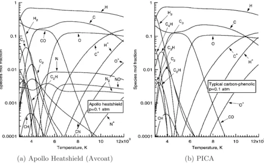
by the ablation of specific components in the heatshield. This translates into a heatshield that is designed to recess upon entry into an atmosphere at hypervelocity speeds. Due to the many complicated physical phenomena occurring when a heat shield starts to ablate, it is difficult to accurately predict the performance of the heatshield (Fig. 1.2). This thesis focuses on phenolic impregnated carbon ablator (PICA) heatshields, as this material is currently being studied and used by NASA, SpaceX, and ESA. This material was first used as the forebody heat shield on the Stardust mission launched in 1999 [159], and was more recently used as the heatshield material for MSL [21]. PICA is a composite material that is formed by combining a porous carbon fiber matrix with a phenolic-resin. As the composite material is heated, the resin begins to thermally degrade at a lower temperature than the fibers. Pyrolysis gases are created as the resin undergoes a thermal decomposition, and these gases flow internal to the heatshield before being injected into the boundary layer above the heatshield. The properties of these pyrolysis gases play a prime role in determining the overall thermal response of the heatshield.
(a) Apollo Heatshield (Avcoat) (b) PICA
Figure 1.4: Example thermodynamic equilibrium gas mixture produced from the Avcoat material used in the Apollo Heatshield (a), and from PICA (b). Figure reproduced from Parket al.[122].
equilibrium calculations are shown using the same elemental composition up to 12000 K. The MSL data analysis predicted a maximum surface temperature of the heatshield to be∼2000 K [21], and simulations performed on sample Earth re-entry trajectories predict maximum surface temperatures to be∼3500 K [108]. Higher temperatures will be found external to the heatshield, but there the gas composition will be a combination of both the pyrolysis gases, and the atmospheric gas. This implies that using a constant elemental composition for all temperatures, as shown in Fig.1.4, is an over-simplification of what is occurring around a re-entry vehicle. Furthermore, little experimental data exists beyond Sykes’ [162] work from the late 1960s, and only recently have preliminary results been shown re-creating these experiments [182].
Chapter 2
Vertical Expansion Tunnel
1
2.1
Motivation
Figure 2.1: Above is a schematic of an expansion tunnel. The states 4 , 1 and 11 are the initial (or fill) conditions of the driver, the intermediate and the accelerator sections, respectively. Below is an x-t diagram of expansion tunnel operation. Shock waves are shown as thick solid lines. Expansion characteristics are shown as thinner solid lines. The contact discontinuities are shown as dashed lines. A particle path (PP), representative of the test gas, is shown as a dashed-dot line.
LD,LI,LA andLN are the lengths of the driver tube, the intermediate tube, the accelerator tube, and the nozzle, respectively. The test time is labeled by∞.
First proposed by Trimpi and Callis [171, 172], the expansion tube and tunnel (ET) have been developed as hypersonic ground-test facilities for approximately half a century. A schematic for the
1
operation of a standard expansion tunnel is shown in Fig.2.1, where each numbered box represents a state in the expansion tunnel. Shock waves are shown as thick solid lines. Expansion characteristics are shown as thinner solid lines. The contact discontinuities are shown as dashed lines. A particle path (PP), representative of the test gas, is shown as a dashed-dot line. LD,LI,LAandLN are the lengths of the driver tube, the intermediate tube, the accelerator tube, and the nozzle, respectively. An expansion tunnel operates ideally as follows: a pressure difference between the driver tube and the intermediate tube is prescribed, and the primary diaphragm is instantly ruptured. The primary contact surface impulsively advances from the primary diaphragm station into the intermediate tube. The impulsive advance of the primary contact surface necessitates a pressure discontinuity that processes the test gas (the primary shock wave). Upon arrival of the primary shock wave at the secondary diaphragm station, the secondary diaphragm instantly ruptures, and a secondary contact discontinuity impulsively advances into the accelerator tube. The impulsive advance of the secondary contact surface necessitates a pressure discontinuity that processes the accelerator gas (the secondary shock wave). Concurrent with the secondary diaphragm rupture, an unsteady expansion (centered at the secondary diaphragm station) processes the test gas. The test gas is accelerated, first through this unsteady expansion, and then (in the case of an expansion tunnel) through the diverging nozzle at the end of the accelerator tube. With the addition of a nozzle, a light tertiary diaphragm is required to separate the accelerator section and the nozzle. As shown in Fig.2.1, the tertiary diaphragm ruptures with the arrival of the secondary shock. This occurs sufficiently far from the test gas that any non-ideal effects associated with this diaphragm rupture will not be a major source of noise during the test time.
In the 1960’s and 1970’s, several expansion tubes and tunnels were constructed and results were reported with significant perturbations in the test flow [102,116,153,158]. The perturbations were likely the result of acoustic waves in the driver gas being transmitted into the test gas and/or non-ideal rupture of the secondary diaphragm. The disruptive acoustic waves that are transmitted to the test gas from the driver gas occur for certain ratios of sound speed across the primary contact surface,
a3/a2 [124,125]. Jacobs [62] used numerical techniques to study the introduction of perturbations
from the driver gas to the test gas. Mitigation of these unsteady sources of noise by appropriate design and operation of an expansion tube has been successfully demonstrated at the University of Illinois at Urbana-Champaign by Dufrene et al. [34]. The effects of the disruptive acoustic waves were decreased by increasing the ratio of the driver pressure to the intermediate pressure (p4/p1),
corresponded to maximum pressure fluctuations of ±50% of the mean value during the test time, which was deemed acceptable from an experimental standpoint.
The non-ideal rupture of the secondary diaphragm can disturb the test gas in three ways: 1) the reduction in useful test time due to finite secondary diaphragm rupture duration [60], 2) the wave system that arises from the reflection of the primary shock wave off the secondary diaphragm can affect the thermo-chemical properties of the gas [10], and 3) the diaphragm particulates can contaminate the test gas by introduction of foreign matter to the test flow [104], reacting with the test gas if the temperature is sufficiently high.
Since the inception of the simple shock tube, significant efforts have been made to understand and mitigate diaphragm rupture issues [42, 126, 146, 154, 180]. Researchers have extended this basis of knowledge to the problems associated with secondary diaphragm rupture in an expansion tube [41, 104, 144, 179]. Furthermore, models of the secondary diaphragm rupture process have been formulated and can be found in the literature [10,115]. The particulates, which travel on the order of the test flow velocity, can also impact and damage the test article [104, 179].
A number of expansion tube/tunnel facilities exist, including the X facilities at the University of Queensland [115], the HYPULSE facility at NASA [38], the JX-1 facility at Tohoku University [150], the 6-inch expansion tube at Stanford University [13,55], the HET facility at University of Illinois at Urbana-Champaign [34], and the LENS X facility at CUBRIC [58]. These facilities have been used successfully for hypersonic aerodynamics and combustion research. Nevertheless, some of the proceedings and articles show results from these facilities with significant test gas perturbations (often conveyed through pressure measurements). In particular, many of these perturbations appear in the vicinity of the test gas/accelerator gas interface; this is evidence of the secondary diaphragm rupture adversely affecting the results. Recent work at Stanford has explicitly shown the effect of impact of secondary diaphragm particulates on pressure measurements [104].
(VET). In the following sections, an overview of expansion tubes/tunnels is provided, a comparison of the available parameter space in a vertical expansion tunnel (VET), an expansion tunnel (ET), and a reflected shock tunnel (RST) is presented. The comparison is restricted to perfect-gas conditions. Perfect-gas quasi-1D Euler computations are used to calculate the available test time in the VET and the ET; in addition, a referenced method is used to calculate the test time in a RST.
2.2
Available Conditions
In this section, a comparison of the parameter space available in a vertical expansion tunnel (VET), conventional expansion tube (ET), and reflected shock tunnel (RST) is presented. The driver pres-sure (p4= 8.16 MPa) is chosen so that it could be filled by conventional research He gas bottles. In
all but one case, the test gas temperature is restricted to be below≈2000 K to ensure a fair compar-ison between facilities and to avoid the detrimental effects of test gas heating [60]. The restriction of maximum test gas temperature permits the perfect-gas assumption. Additionally, at the pressure ratio specified in Table 2.1, (p4/p1 ≈1000), the sound speed ratio is a3/a2 ≈0.57; at this a3/a2,
Dufreneet al. [34] observed experimentally that the Paull and Stalker type [125] perturbations in the free-stream were acceptable. To aid in comparison, the test gas in each facility is expanded to a free-stream Mach number of 5.5. In the VET, this necessitates the use of a nozzle at the end of the expansion tube to increase the Mach number, making it an expansion tunnel. Without a nozzle for the VET, useful test conditions cannot be created. A nozzle is not needed at the end of the conventional ET because of the more efficient unsteady expansion.
Pressure-velocity diagrams are used to find the conditions of the test gas as it is processed by the wave systems (for reference, follow the particle path, PP, in Fig.2.1). The static pressure and velocity must be matched in states 2 and 3 and in states 12 and 13 . This is done by plotting the expansion
p3
p4
=
1−(γ4−1)(2au3−u4)
4
2γ4 γ4−1
, (2.1)
and shock relationships
u2−u1
a1
= p2−p1
γ1p1
q
1 +(γ1+1)(2γ1p1p2−p1)
, (2.2)
in pressure - velocity space and finding the point of intersection [87]. Here,γ is the ratio of specific heats, p is the static pressure, u is the velocity, and a is the sound speed. Eq. 2.1 and Eq. 2.2
equations that would be used to evaluate the states 12 and 13 . In the VET, the gas from state 13 is expanded through a nozzle using the usual steady quasi-1D gas-dynamic equations.
0 2 4 6 8 10
10−2 10−1 100 101 102 103 104
u/a
1p
/
p
12,3
12,13(
∞
)
11
4
1
EW
4→3
SW
1→2
EW
2→13(∞)
SW
11→12
Figure 2.2: Pressure-velocity diagram for a conventional expansion tube. Expansion waves are denoted by EW, and shock waves are denoted by SW. Note that 13(∞) denotes the free-stream state.
0 2 4 6 8
10−1 100 101 102 103 104
u/a
1p
/
p
12,3
12,13
∞
4
1,11
EW
4→3
SW
1→2
EW
2→13
SW
11→12
SE
13→∞
Figure 2.3: Pressure-velocity diagram for a vertical expansion tunnel. Expansion waves are denoted by EW, shock waves are denoted by SW, and the steady expansion is denoted by SE. Note that ∞ denotes the free-stream state.
the accelerator gas by density stratification (pressure-velocity diagram in Fig. 2.3). The unsteady expansion centered at the secondary diaphragm station is stronger in the ET when compared with the VET; for this reason, the conventional ET is able to reach higher effective reservoir states than the VET. If some sacrifice of the reservoir conditions can be made, the VET can be utilized in hypervelocity ground testing without the problems associated with secondary diaphragm rupture.
The available conditions and test times for a given set of fill pressures are tabulated (Table2.1) for three types of impulse hypersonic facilities, the VET, the ET, and the RST. The effective reservoir conditions (reservoir pressure and mass specific enthalpy) for the conventional ET and the VET are found by isentropic compression of state 13 to rest. The pressure,p1, for the first shock tunnel case
(RST-1) is chosen such that it is operated in the tailored mode. The pressure,p1, for the second
shock tunnel case (RST-2) is chosen so that the temperature in the test gas does not exceed 2000 K. At this pressure ratio (p4/p1), the RST will be operated in an over-tailored mode, and the Mach
number of the primary shock is 10% higher in RST-2 relative to the tailored condition (RST-1). The pressure, p1, for the third shock tunnel case (RST-3) is chosen such that the reservoir mass
specific enthalpy is matched to the VET case and requires a 50% increase in the Mach number of the primary shock relative to the tailored condition (RST-1). In this case, the test gas will be reacting, so Cantera [47] with the Shock and Detonation Toolbox [25] is used to evaluate the conditions in the reservoir and through the nozzle. The appropriate thermodynamic data [50,100] and reaction rates [53] are found in the literature. The test gas is assumed to be in chemical equilibrium in the reservoir and up to the throat of the nozzle. The run conditions at the nozzle exit are found by the integration of a system of coupled ordinary differential equations (accounting for finite-rate chemistry) from the throat to the nozzle exit; the equations are derived in [69]. At matched reservoir mass specific enthalpy, the VET has a higher effective reservoir pressure than in the RST-3 case. This performance advantage of the VET relative to the RST would become increasingly apparent by increasing the local Mach number in state 2 because the total temperature and pressure gain in an unsteady expansion varies strongly with Mach number. In the RST-3 case there is 3.5% NO (by
Table 2.1: Comparison of run conditions available for a reflected shock tunnel (RST), conventional expansion tunnel (ET), and a vertical expansion tunnel (VET).2
mole) in the free-stream (calculatedusing Cantera [47] with the Shock and Detonation Toolbox [25]); all other cases in all facilities produce a negligible amount of NO.
If the quantity of interest in ground-test facilities is effective reservoir conditions, then the capa-bility of the VET is above the RST, but below the ET. One advantage of the ET or VET over the shock tunnel is a lower maximum test gas temperature for a given reservoir mass specific enthalpy, so the detrimental effects of the test gas being partially dissociated and partially vibrationally excited are less severe. To increase test time one can scale the facility size up; however, in the case of a RST nozzle throat heating will become a problem long before the problem would become apparent in the ET or VET [60].
2.3
Test Time Calculation for the RST and ET
Test time calculations for the facilities shown in Table2.1require facility sizing choices to be made. AnL/d(1.27 m/25.4 mm) ratio of 50 is chosen to minimize the effects of the boundary layer on the walls of the shock tube [109]; and is held constant for the RST, ET, and VET for comparison. The overall length is chosen so that it may fit into a single story lab as a demonstrator-type facility.
In the RST, a 10◦ half angle nozzle of throat diameter 8.46 mm (1/3 in), length 175 mm,
and area ratio 70 is chosen so that the test section is of similar size to the VET. The test time (listed in Table2.1) was considered to begin after the nozzle startup time (estimate formulated by Smith [156]) and end after the driver gas contaminates the test gas (estimate formulated by Wilson and Davies [32]). This methodology to estimate the test time has been successfully demonstrated by Sudani and Hornung [161].
0
0.2
0.4
0.6
0
200
400
600
x
, m
t
,
µ
s
Test Time
Expansion Head
Transmitted Shock
Secondary CD
Expansion Tail
Re
fl
ected Expansion Head
Primary CD
Figure 2.4: Schematic x-t diagram for a conventional ET, focusing on the accelerator tube, and the ideal test time.
observed test times in expansion tunnels will be provided in Sec.2.5.2. Within the framework of these idealized calculations, increasing the test time of the facility simply requires an increase in the facility length, as the test time scales linearly with combined length of the intermediate and accelerator sections.
Calculation of the ideal test time in the VET requires the consideration of the location and length of the nozzle, both of which significantly affect the test time. Unfortunately, no analytical results are available when a nozzle is present. To explore a large parameter space at a relatively low computational cost, quasi-1D Euler computations are performed based on a method suggested by Glaister [45]. A summary of this method is presented in the following section, followed by the results.
2.4
Ideal Test Time Calculation for the VET
temperatures reached by the gases throughout the different states, this is a valid assumption. In addition, it is assumed that there is no mixing between any of the gases at the fluid interfaces as a result of the short run time. A discussion of non-idealized effects associated with expansion tunnels will be provided in Sec.2.5.
2.4.1
The Compressible Euler Equations with Area Change
Following the method of Glaister [45], in three dimensions, and in a general orthogonal coordinate system given by (x1, x2, x3), the Euler equations are given by Eqs.2.3—2.5.
ρt+∇ ·(ρu) = 0 (2.3)
(ρu)t+∇ ·(ρuu) = −∇p (2.4)
et+∇ ·[u(e+p)] = 0 (2.5)
Combining these with Eq.2.6, the equation of state for an ideal gas, allows the flow of an unsteady compressible inviscid fluid to be solved for.
e= p
γ−1+ 1
2ρu·u (2.6)
Here,ρ=ρ(x, t),p=p(x, t),e=e(x, t), andu=u(x, t) = [u1(x, t), u2(x, t), u3(x, t)]T represent
the density, pressure, total energy, and the three components of velocity, respectively, at a general position in space given by x= (x1, x2, x3)T and at time t. The divergence and gradient operators
are left in a general form, and to evaluate these equations, the appropriate operator must be used based on the chosen coordinate system.
In a general 3D orthogonal coordinate system, a line element dscan be written as
ds=ξ1dx1ˆx1+ξ2dx2xˆ2+ξ3dx3ˆx3, (2.7)
where ξ1, ξ2, andξ3 are scalar lengths. In Eq.2.7,xˆ1, ˆx2, and ˆx3 are the unit vectors parallel to
their specific coordinate lines. Assuming an ideal nozzle, all changes in the flow depend only on one coordinate direction. In this case, it is assumed that all variables are a function of only x1 andt,
where the x1 coordinate corresponds to the location along the centerline of the nozzle. It is now
possible to write u= [u(x1, t),0,0]T =u, which is a parallel flow assumption, and is only valid for
can be re-written as follows
(ξ1ξ2ξ3ρ)t+ (ξ2ξ3ρu)x1 = 0 (2.8)
(ξ1ξ2ξ3ρu)t+ (ξ2ξ3ρu2)x1 = −ξ2ξ3
∂p
∂x1 (2.9)
(ξ1ξ2ξ3e)t+ [ξ2ξ3u(e+p)]x1 = 0 (2.10)
In order to describe compressible fluid flow through a duct of smoothly varying cross section, ξ1
can be an arbitrary constant, and here it is assumed thatξ1= 1. Using this assumption, it is now
possible to once again rewrite the Euler equations as
(ξ2ξ3ρ)t+ (ξ2ξ3ρu)x1 = 0 (2.11)
(ξ2ξ3ρu)t+ [ξ2ξ3(p+ρu2)]x1 = p ∂
∂x1(ξ2ξ3) (2.12)
(ξ2ξ3e)t+ [ξ2ξ3u(e+p)]x1 = 0 (2.13)
In the above equations, the left hand side is similar to the 1D compressible Euler equations in conservative form, while there is an additional source term added to the right hand side that is not present in the classic 1D Euler equations. In order to simplify these equations further, Glaister uses the notationS(r) = ξ1ξ2, so thatS(r) represents the cross-sectional area of the duct at a point r,
whereris the distance in thex1 direction. This system of equations can then be written as
[S(r)w]t+ [S(r)f(w)]r=g(w), (2.14)
where w= ρ ρu e
, f(w) = ρu
p+ρu2
u(e+p)
and g(w) = 0
pS′(r)
0 . (2.15)
Wt+ [F(W)]r=g(w), (2.16)
where W = S(r)w. Following the terminology used by Glaister, this gives rise to a new set of “conserved” variables; R, E, and P. R = S(r)ρ, E = S(r)e and P =S(r)p. It is important to note that with these new conserved variables, the gas velocity, speed of sound, and enthalpy remain the same: U =u, a=p
γp/ρ=p
γP/R, andh= (e+p)/ρ= (E+P)/R=H. In addition, the Jacobian remains unchanged:
A= ∂F(W)
∂W =
∂f(w)
∂w . (2.17)
Finally, the Euler equations for duct flow are written as
R RU E t + RU
P+RU2
U(E+P) = 0 PS ′ (r)
S(r)
0 . (2.18) with
E= P
γ−1 + 1 2RU
2. (2.19)
2.4.2
Roe Solver
A standard Roe Riemann Solver [145] is used to solve these equations. To denote Roe averaged values, the notation ˜Y is used, where
˜
Y = √
RLYL+√RRYR √
RR+√RL
. (2.20)
L and R refer to the left and right cell values, as the averaged quantities are calculated at cell interfaces. The eigenvalues ofA˜ can be calculated to be
˜
λ(1)= ˜U−˜a, ˜λ(2) = ˜U , λ˜(3)= ˜U+ ˜a (2.21)
with corresponding eigenvectors of
˜e(1) = 1 ˜
U−˜a
˜
H−U˜˜a
, ˜e(2)= 1 ˜ U 1 2U˜
2
and ˜e(3)= 1 ˜
U + ˜a
˜
where ˜a= (γ−1)( ˜H−12U˜ 2).
A numerical approximation for ˜g(w) must be used, and Glaister proposed that
˜
g2(wn) =
Sj−Sj−1
∆r
˜
ρ˜a2
γ (2.23)
is a natural choice for this approximation. Here,Sj represents the average cross sectional area over cellj. With this notation, it is easy to see that to go from this new set of conserved variables to the more traditional set of conserved variables, the simple relation ofwn
j =
Wnj
Sj must be used.
The fluxes are projected onto the eigenvectors of the system so that a standard explicit update step can be employed. In addition to the standard wave strengths being obtained for the Euler equations, ˜g(wn) is also projected onto the eigenvectors which modifies the standard wave strengths that result from the Euler equations. Cell values are updated using a flux difference splitting method which is outlined in Eq.2.24.
Wnj+1=Wnj − ∆t ∆r X ˜
λ(i) j+ 12≤0
˜
λ(ji+)1 2 ˜
γj(i+)1 2 ˜ e(ji+)1
2
+ X
˜
λ(i) j−1
2
≥0
˜
λ(ji−)1 2 ˜
γj(i−)1 2 ˜ e(ji−)1
2 (2.24)
Here, the summations are performed over i, where i = 1,2,3. The subscripts refer to the cell interface (j±1/2) where each value is calculated, the regular superscripts (n) correspond to a time step, and the superscripts in brackets (i) correspond to a component (i∈1,2,3).
Additionally, ˜γ(i) refers to the modified wave strength, where
˜
γ(i)= ˜α(i)+ ˜β(i)/λ˜(i). (2.25)
The ˜α(i) wave strengths are the standard Roe-averaged wave strengths, where
˜
α(1)= 1
2˜a2(∆rP −R˜˜a∆rU), α˜
(2)= ∆r
R −∆rP˜a2 and α˜
(3)= 1
2˜a2(∆rP+ ˜R˜a∆rU). (2.26)
The ∆r operator is the difference in value between different cells, so that ∆rUj+1/2 =Uj+1−Uj.
The ˜β(i)in Eq.2.24takes into account changes in cross sectional area and can be expressed as
˜
β(1)= R˜∆rS
2γS˜ [(γ−1) ˜U+ ˜a],
˜
β(2)=−(γ−1) ˜RU˜∆rS
γS˜ , and
˜
β(3)= R˜∆rS
Figure 2.5: Schematic for the flux correction suggested by Abgrall and Karni when dealing with an interface between two different fluids.
where ˜Sj+1/2=
p
Sj+1Sj.
2.4.3
Treatment of Fluid Interfaces
The above numerical method assumes thatγis constant for every cell in the domain. This is not true for the present investigation. It is possible to create unphysical oscillations at the interface between two different fluids if no special care is taken when calculating values at these fluid interfaces. A modification to the above scheme is used that was originally suggested by Abgrall and Karni [7].
Abgrall and Karni [7] suggested that a way to avoid unphysical oscillations at fluid interfaces is to calculate two separate fluxes between the different fluids. A schematic explaining this method is shown in Fig. 2.5, where the cell face atj+1
2 is the interface between two different fluids with
two different ratios of specific heats, γ1 and γ2, respectively. When updating cell j, γ1 is used to
calculate the properties needed atj+1
2, and when updating cellj+ 1,γ2 is used to calculate the
values needed atj+12. In addition, the order in whichγvalues are updated in the domain based on a scalar transport equation need be performed carefully. A more detailed explanation can be found in Abgrall and Karni’s original work [7].
The drawback is that this scheme no longer conserves total energy since two different fluxes are calculated at the same interface. In addition, the scheme uses “frozen” thermodynamics, orγvalues from the previous time step to calculate the new values. Abgrall and Karni [7] show that across a material interface where pressure and velocity are constant (a standard contact discontinuity), the errors induced due to the different fluxes used and the lag in updating γ are actually opposite in sign, and very similar in magnitude. In addition, there are only three material interfaces in the current simulations, and these interfaces are the only places where total energy is not conserved. When the number of grid points in the domain is increased, the relative loss of total energy reduces. It has been checked that the loss of total energy in the simulations run for this investigation were negligible (<0.001%).
φis a passive scalar.
∂φ ∂t +u
∂φ
∂x = 0 (2.28)
The levelset function,φ, is used to determine the location of the different gases. For the case where the driver and accelerator gases are the same and the test gas is different, it is simple to assignφan initial value of 1 in the driver and accelerator sections, and a value of -1 in the intermediate section. If a nozzle is used, it is assumed that the nozzle will be filled with low pressure air, and therefore
φ is this section is also assigned a value of -1. After advecting φ, a hard switch is employed such that if φ≥0, the properties of driver/accelerator gas are used; and if φ < 0, the properties of the intermediate gas are used. A modified form of the semi-Lagrangian scalar scheme discussed in [136] is used to solve the scalar advection equation. Traceback of the grid-node particles is achieved using first-order backward Euler time integration. A 5th-order accurate Lagrange polynomial is used for interpolating the scalar at the traced-back location. A switch to monotonicity preserving first-order linear interpolation is triggered if the interpolated scalar value breaches physical bounds.
2.4.4
Higher-Order Corrections
The numerical scheme explained in Section 2.4.2is at best first order and diffusive, which means shocks and contact discontinuities are unphysically spread over many grid cells. To help alleviate this problem, a higher-order flux correction is added using wave limiters [84]. In order to implement this, an additional term is added to Eq.2.24, so that it is modified to
Wjn+1=Wjn− ∆t ∆r X ˜
λ(i) j+ 12≤0
˜
λ(ji+)1 2˜γ
(i)
j+1 2e˜
(i)
j+1 2 +
X
˜
λ(i) j−1
2
≥0
˜
λ(ji−)1 2γ˜
(i)
j−1 2˜e
(i)
j−1 2 − ∆t
∆r(Fˆj+12− ˆ Fj−1
2), (2.29)
with
ˆ Fj−1
2 = 1 2 3 X i=1
|λ˜(ji−)1 2|
1−∆∆rt|˜λ(ji−)1 2|
˜ Bj(i−)1
2. (2.30)
˜ B(ji−)1
2 = Φ(θ
(i)
j−1 2)B
(i)
j−1
2, where Φ(θ) is a limiting function, and B
(i)
j−1 2 = ˜α
(i)
j−1 2e˜
(i)
j−1
2. A Van Leer limiting function is used [173]:
Φ(θ) = θ+|θ|
1 +θ . (2.31)
≈1000 between the driver gas and intermediate gas creates extremely steep gradients and rapidly changing eigenvectors. Lax and Liu [81] suggested a robust function forθ that is designed to work with systems of non-linear equations. They define
θ(ji−)1 2 =
ˆ BJ(i−)1
2· B
(i)
j−1 2 Bj(i−)1
2 · B
(i)
j−1 2
, (2.32)
where
ˆ BJ(i−)1
2 = (˜l
(i)
j−1 2∆WJ−
1 2)˜e
(i)
j−1
2, (2.33)
and˜lis the appropriate left eigenvector using Roe-averaged quantities. In addition,J changes value based on the sign of the eigenvector, so that the limiting is performed in an upwinded or downwinded manner as necessary, so
J =
j−1 if ˜λ(ji−)1 2 >0
j+ 1 if ˜λ(ji−)1 2
<0.
(2.34)
These higher-order corrections do a good job at making both contact discontinuities and shocks sharper in the simulations. The flux limiters are not used in the vicinity of walls, or at the interface between two fluids with different values ofγ.
2.4.5
Entropy Fix
Due to the large pressure ratios needed initially in order to achieve relevant test conditions, an entropy fix is required to avoid entropy-violating (expansion) shocks in the solution. The entropy fix proposed by Sanderset al.[149] is implemented, and no entropy violating solutions are observed.
2.4.6
Numerical Results: Verification
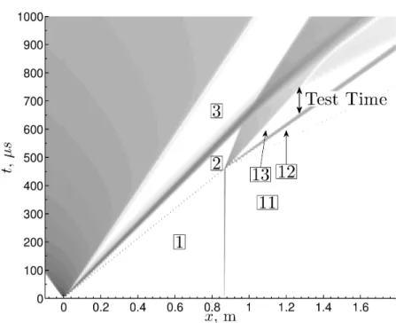
A 1D perfect-gas Euler computation with the same initial conditions as the proposed VET but
Figure 2.6: Numerical x-t diagram for a 1D perfect gas Euler simulation with the same initial conditions as the proposed VET.
intermediate and accelerator sections is atx= 0.86 m.
To visualize the results of the 1D perfect-gas Euler computations, a numerical x-t diagram is made using a numerical schlieren method, where contours of the function−log(|∂x1∂ρ|) are plotted (Fig.2.6). The simulation results capture the theoretical wave system depicted in Fig.2.1. There is also good quantitative agreement between the numerical results and the analytical solution. The numerical results differ from the analytical results by no more than the third significant digit (≈ 0.5%) for pressure, velocity or density in states 2 and 3 and states 12 and 13 . The numerical values have been averaged over the respective appropriate section, att= 450µs for states 2 and 3 and att= 600µs for states 12 and 13 .
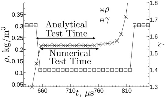
Comparison of the test time between the 1D perfect gas Euler simulations and the analytic calculations is also necessary to fully validate the numerical technique. The numerical test time is defined to be when the density is within 1% of the average value of density in the constant region, state 13 . Figure 2.7 shows a comparison between the analytic test time and the numerical test time. While fluctuations during the test time in an experimental facility are expected to be much larger than 1%, we note that these analyses are for validation of the numerical technique.
0.05
0.1
0.15
0.2
0.25
0.3
0.35
Numerical
Test Time
Test Time
Analytical
ρ
,
k
g
/
m
3
660
710
760
810
1.3
1.4
1.5
1.6
1.7
1.8
t
,
µ
s
γ
ρ
γ
Figure 2.7: Comparison between the analytic test time and the numerical test time for the 1D case.
case, are spread out over a few cells in simulations due to numerical diffusion. In addition, the reflection of waves off of a contact discontinuity of finite thickness may introduce errors in the simulations. Nevertheless, these small differences are acceptable, so quasi-1D Euler simulations are started with the addition of the nozzle at the end of the accelerator tube.
2.4.7
Numerical Results: VET with Nozzle
The addition of a nozzle at the end of the accelerator tube is necessary for useful test conditions to be generated with the VET. The addition of a nozzle also expands the design parameter space that must be investigated. In this analysis, we consider changes to the location of the nozzle and lengths of the intermediate and accelerator sections. The sum of the intermediate and accelerator section lengths is still subject to the constraintL/d= 50. The same initial conditions as the proposed VET (Table 2.1) were used. A 10◦ conical nozzle of length L
Figure 2.8: Numerical x-t diagram for an expansion tunnel with a 10◦ half angle diverging conical
1
1.05
1.1
1.15
1.2
55
60
65
70
75
80
85
90
T
es
t
T
im
e,
µ
s
L
I,nozzle
/L
I,
1
D
Figure 2.10: Test time for varying lengths of the intermediate and accelerator sections when using a nozzle.
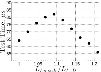
VET (Table2.1). An unsteady expansion is created when the secondary contact discontinuity enters the nozzle. The trailing characteristic from this unsteady expansion corresponds to the beginning of the test time. The test time is ended when either the tail or reflected head of secondary expansion wave reaches the test location. The qualitative behavior of the nozzle startup processes observed in Fig.2.9are consistent with the features seen in previous studies on nozzle start up phenomenon [156]. The predicted test time changes with the intermediate and accelerator lengths (Fig.2.10). For all cases, the intermediate and accelerator section length sum is held constant at 1.27 m. LI,nozzle refers to the length of the intermediate section when a nozzle is used, and this length is normalized byLI,1D, the ideal intermediate section length when no nozzle is used (LI,1D= 0.86 m). Increasing the intermediate section length (and reducing the accelerator section length) - with respect to the 1D case - increases the test time. After a certain threshold, the test time starts to decrease. All points to the left of the maximum t
![Table 1.1: Summary of successful NASA Mars landers and rovers. Data taken from [ 37 ] and NASA- NASA-JPL press releases made available to the public [ 2 , 3 , 4 , 5 , 6 ].](https://thumb-us.123doks.com/thumbv2/123dok_us/1124594.1141411/16.918.171.807.925.1039/table-summary-successful-landers-rovers-releases-available-public.webp)