Wackersreuther, Bianca (2011): Efficient Knowledge Extraction from Structured Data. Dissertation, LMU München: Fakultät für Mathematik, Informatik und Statistik

(1)

Efficient Knowledge Extraction

from Structured Data

Bianca Wackersreuther

(2)

(3)

Efficient Knowledge Extraction

from Structured Data

Bianca Wackersreuther

Dissertation

an der Fakult¨at f¨ur Mathematik, Informatik und Statistik

der Ludwig–Maximilians–Universit¨at

M¨unchen

vorgelegt von

Bianca Wackersreuther

aus F¨ussen

(4)

Erstgutachter: Prof. Dr. Christian B¨ohm

Zweitgutachter: Prof. Dr. Thomas Seidl

(5)

(6)

(7)

Acknowledgments

I would like to express my warmest gratitude to all the people who supported me during the past four years while I have been working on this thesis. I avail myself of the opportunity to thank them, even if I cannot mention all of their names here. First of all, I would like to express my warmest and sincerest thanks to my supervisor, Professor Dr. Christian B¨ohm. The joy he has for his research was contagious and motivational for me, even during tough times. I warmly acknowl-edge Professor Dr. Thomas Seidl for his immediate willingness to act as a second referee for my thesis. I would also like to thank the other two members of my oral defense committee, Professor Dr. Claudia Linnhoff-Popien and Professor Dr. Rolf Hennicker, for their time and insightful questions.

(12)

xii Acknowledgments

Dr. Karsten Borgwardt was an awesome teacher of mine for the field of graph mining. It has been a unique chance for me to learn from his scientific experience and his never-ending enthusiasm for his research.

I have appreciated the database research group of the LMU. I am grateful to our chair secretary, Susanne Grienberger and our group’s administrative assistant Franz Krojer who kept us organized and were always ready to help.

I was honored to be a mentee of the LMU Mentoring program. Professor Dr. Francesca Biagini always supported my work and has been a dedicated mentor to me.

Lastly, I would like to thank my family and my friends for all their love and encouragement, and most of all my loving, encouraging, and patient husband Pe-ter whose faithful support during the final stages of this thesis is so appreciated. Thank you!

(13)

Abstract

Knowledge extraction from structured data aims for identifying valid, novel, po-tentially useful, and ultimately understandable patterns in the data. The core step of this process is the application of a data mining algorithm in order to produce an enumeration of particular patterns and relationships in large databases. Clustering is one of the major data mining tasks and aims at grouping the data objects into meaningful classes (clusters) such that the similarity of objects within clusters is maximized, and the similarity of objects from different clusters is minimized.

(14)

xiv Abstract

a local optimum by a beneficial combination of genetic algorithms, information theory and model-based clustering. Besides hierarchical data mining, we also made contributions to more complex data structures, namely objects that consist of mixed type attributes and skyline objects. The algorithm INTEGRATE performs integrative mining of heterogeneous data, which is one of the major challenges in the next decade, by a unified view on numerical and categorical information in clustering. Once more, supported by the MDL principle, INTEGRATE guaran-tees the usability on real world data. For skyline objects we developed SkyDist, a similarity measure for comparing different skyline objects, which is therefore a first step towards performing data mining on this kind of data structure. Applied in a recommender system, for example SkyDist can be used for pointing the user to alternative car types, exhibiting a similar price/mileage behavior like in his orig-inal query. For mining graph-structured data, we developed different approaches that have the ability to detect patterns in static as well as in dynamic networks. We confirmed the practical feasibility of our novel approaches on large real-world case studies ranging from medical brain data to biological yeast networks.

(15)

Zusammenfassung

Das Ziel der Wissensgewinnung aus strukturierten Daten ist es, gültige, bislang unbekannte, potentiell nützliche und letztendlich verständliche Muster in den Daten aufzudecken. Zentraler Schritt dieses Prozesses ist die Anwendung eines sog.

Data MiningAlgorithmus, der eine Aufzählung bestimmter Muster und Beziehun-gen in großen Datenbanken erzeugt. Eine wichtige Aufgabe des Data Minings stellt das sog. Clustering dar. Dabei sollen die Datenobjekte so in Gruppen (Cluster) zusammengefasst werden, dass die Ähnlichkeit aller Objekte innerhalb eines Clusters maximiert und die Ähnlichkeit der Objekte unterschiedlicher Clus-ter minimiert wird.

(16)

Datenkom-xvi Zusammenfassung

primierung im Sinne derHuffman Codierungeingesetzt werden. Daher stellt die theoretisch erreichbare Komprimierungsrate eine natürliche Zielfunktion für das Clustering-Problem dar, die automatisch alle vier zuvor genannten Zielsetzun-gen erfüllt. Der Zielsetzun-genetische hierarchische Clustering-Algorithmus GACH (Genetic Algorithm for finding Cluster Hierarchies) beseitigt das Problem, ein lediglich lokales Optimum als endgültige Lösung zu finden, durch eine geschickte Kombi-nation von genetischen Algorithmen, Informationstheorie und Modell-basiertem Clustering. Neben dem hierarchischen Data Mining, widmeten wir uns auch kom-plexeren Datenstrukturen, nämlich Objekten, die durch Attribute unterschiedlichen Typs repräsentiert sind sowie Skyline-Objekten. Der Algorithmus INTEGRATE setzt die integrative Analyse heterogener Daten um, was sich als eine der Haup-taufgaben für die nächsten Jahrzehnte herausgestellt hat, indem er sowohl die nu-merische als auch die kategorische Information für den Clustering-Prozess vere-int berücksichtigt. Auch in diesem Fall garantiert INTEGRATE, unterstützt durch das MDL Prinzip, den praktischen Einsatz für reelle Daten. Für Skyline-Objekte haben wir das Ähnlichkeitsmaß SkyDist entwickelt, welches den Vergleich unter-schiedlicher Skyline-Objekte erlaubt und damit einen ersten Schritt in Richtung Data Mining auf dieser Art von strukturierten Daten darstellt. Eingesetzt in einer priorisierten Suchmaschine, kann SkyDist beispielsweise dazu verwendet werden, dem Nutzer unterschiedliche Autotypen vorzuschlagen, die entsprechend dem in der Anfrage spezifizierten Preis/Kilometerstand Profil ähnliche Eigenschaften aufweisen. Zur Analyse Graph-strukturierter Daten haben wir unterschiedliche Ansätze entwickelt, die sowohl in statischen als auch in dynamischen Netzwerken zum Auffinden von Mustern herangezogen werden können. Wir belegten die prak-tische Anwendbarkeit unserer neuen Ansätze an großen realen Fallstudien, die von medizinischen Gehirndaten bis hin zu biologischen Hefe-Netzwerken reichen.

(17)

Zusammenfassung xvii

Grafikverarbeitung in leistungsstarke Co-Prozessoren entwickelt, die sich nicht mehr nur für typische Grafikaufgaben eignen, sondern mittlerweile auch für all-gemeine numerische und formale Berechnungen verwendet werden können. Der Hauptvorteil der GPUs liegt darin, dass sie extrem starke Parallelität und gleich-zeitig hohe Bandbreite im Speichertransfer zu niedrigen Kosten bieten. In dieser Arbeit schlagen wir unterschiedliche Algorithmen für rechenintensive Data Min-ing Aufgaben, wie z.B. der Ähnlichkeitssuche und unterschiedliche Clustering-Paradigmen vor, die speziell auf die hoch parallele Arbeitsweise einer GPU aus-gelegt sind, bezeichnet mit CUDA-DClust und CUDA-k-means. Wir definieren eine multidimensionale Indexstruktur, die so konzipiert wurde, dass sie ¨ Ahnlich-keitsanfragen auch unter dem eingeschränkten Programmierungsmodell der GPU unterstützt und zeigen die Überlegenheit unserer Algorithmen auf der GPU

(18)

(19)

Chapter 1 Preliminaries

(20)

2 1. Preliminaries

Data

Selection

Pre-processing

Trans-formation Data Mining

Patterns

Interpretation / Evaluation

Knowledge

Figure 1.1: The KDD process.

1.1 The Classic Definition of KDD

The classic definition of KDD by Fayyadet al. from 1996 describes it as “the non-trivial process of identifying valid, novel, potentially useful, and ultimately understandable patterns in data” [32]. The KDD process, as illustrated in Fig-ure 1.1, consist of an iterative sequence of the following steps:

1. Selection: Creating a target dataset by selecting a dataset or focusing on a subset of variables or data samples on which discovery is to be performed.

2. Preprocessing: Performing data cleaning operations, such as removing noise or outliers if appropriate, handling missing data fields, accounting for time-sequence information, as well as deciding DBMS issues, such as data types, schema and mapping of missing and unknown values.

3. Transformation: Finding useful features to represent the data depending on the goal of the task, e.g., using dimensionality reduction or transformation methods to reduce the number of attributes or to find invariant representa-tions for the data.

(21)

1.2 Data Mining: The Core Step of Knowledge Extraction 3

5. Interpretation and Evaluation: Applying visualization and knowledge re-presentation techniques to the extracted patterns, and removing redundant or irrelevant patterns and translating the useful ones into terms understandable by users. The user may return to previous steps of the KDD process if the results are unsatisfactory.

1.2 Data Mining: The Core Step of Knowledge

Ex-traction

Since data mining is the core step of the KDD process, the termsKDDandData Mining are often used as synonyms. In [32], data mining is defined as a step in the KDD process which consists of applying data analysis algorithms that, under acceptable computational efficiency limitations, produce a particular enumeration of patterns over the data.

(22)

sum-4 1. Preliminaries

marization and comparison of general features of objects. Frequent itemset and association rule mining focuses on discovering rules showing attribute value con-ditions that occur frequently together in a given dataset. And evolution analysis models trends in time related data that evolve.

1.3 Clustering: One of the Major Data Mining Tasks

In this thesis, we mainly focus on clustering techniques w.r.t. the special chal-lenges posed by complex structured data. The goal of clustering is to find a natural grouping of a dataset such that data objects assigned to a common group called

clusterare as similar as possible and objects assigned to different clusters differ as much as possible. Consider for example the set of objects visualized in Figure 1.2. A natural grouping would assign the objects to two different clustersblueandred. Two outliers not fitting well to any of the clusters should be left unassigned.

Figure 1.2: Example for clustering consisting of two clusters blue and red and two outlier objects.

(23)

1.3 Clustering: One of the Major Data Mining Tasks 5

Curvature Labellum

Color

Length-Sepal(M)

Curv

atur

e

La

bellum

Feature-Transformation

feature vector

Figure 1.3: Example for feature transformation. Five features are measured and transformed into a 5-dimensional vector space.

of the data (e.g. learning thenaturalstructure of data which should be reflected by a meaningful clustering). In other cases, cluster analysis is merely a first step for different purposes such as indexing or data compression. While clustering in gen-eral is a rather dignified problem, mainly in about the last decade new approaches have been proposed to cope with new challenges provided by modern capabilities of automatic data generation and acquisition in more and more applications pro-ducing a vast amount of high dimensional data. These data need to be analyzed by data mining methods in order to gain the full potentials from the gathered informa-tion. However, structured data pose different challenges for clustering algorithms that require specialized solutions. So, this area of research has been highly active in the recent years with an abundance of proposed algorithms.

Like most data mining algorithms, the definition of clustering requires spec-ifying some notion of similarity among objects. In most cases, the similarity is expressed in a vector space, called thefeature space. In Figure 1.2, we indicate the similarity among objects by representing each object by a vector in 2-dimensional space. Characterizing numerical properties (from a continuous space) are ex-tracted from the objects, and taken together to a vector x ∈ _Rd _where _d _{is the}

(24)

6 1. Preliminaries

where the object is a certain kind of an orchid. The phenotype of orchids can be characterized using the lengths and widths of the two petal and the three sepal leaves, of the form (curvature) of the labellum, and of the colors of the different compartments. In this example, five features are measured, and each object is thus transformed into a 5-dimensional vector space. To detect the similarity among two data objectsxandyrepresented as feature vectors, a metric distance functiondist is used. More specifically, letdist be one of the Lp norms, which is defined as

follows for an arbitraryp∈_N.

dist(~x, ~y) = p

v u u t

d

X

i=1

|xi −yi|p

Usually the Euclidean distance is used, i.e. p= 2. If we have more complex data types, we have to define a suited distance function.

For complex data objects, such as images, protein structures or text data, it is a non-trivial task to define domain specific distance functions. In Chapter 5, we introduce SkyDist, a similarity measure for skyline objects. Skyline objects rep-resent a set of data objects that fit to a certain kind of query. The classic example is a user looking for cheap hotels which are close to the beach. Typically, it is unknown to the system how important the two conditions, distance and price, are to the user. The skyline query returns all offers which may be of interest. This means, the skyline does not only contain the cheapest hotel and the hotel closest to the beach but also all hotels providing an outstanding combination ofpriceand distance, which makes them more attractive to the user than any other hotel in the database. The high expressiveness of skylines aims at performing data mining on such data structures.

1.4 Information Theory for Clustering

(25)

1.4 Information Theory for Clustering 7

the number of clusters, density thresholds or neighborhood sizes. In practice, the best way to cope with this problem often is to run the algorithm several times with different parameter settings. Thereby, suitable values for the parameters can be learned in a trial and error fashion. But it is obvious, that this is an extremely time consuming approach. And anyhow, it cannot guarantee that at least useful values for the parameters are obtained.

A beneficial solution for that problem is to relate clustering to data compres-sion. Imagine you want to transfer a dataset consisting of feature vectors via an extremely expensive and small-banded communication channel from a sender to a receiver. Without clustering, each coordinate needs to be fully coded by trans-forming the numerical value into a bit string. But, if the data provides regularities, clustering can drastically reduce communication costs. For example a model-based clustering algorithm, like EM [27], can be applied to determine a statistical model for the dataset, which defines more or less likely areas of the data space. With this knowledge, the data can be compressed very effectively since only the deviations from the model need to be encoded which requires much less bits than the full coordinates. The model can be regarded as a codebook which allows the receiver to de-compress the data again. Following the idea of (optimal) Huffman coding, we assign few bits to points in areas of high probability and more bits to areas of low probability. The interesting observation is the following: the com-pression becomes the more effective, the better our statistical model fits to the data.

(26)

8 1. Preliminaries

developed by different communities include the Bayesian Information Criterion (BIC), the Aikake Information Criterion (AIC) and the Information Bottleneck method (IB) [95].

In Chapter 3, we define a hierarchical variant of the MDL principle, called hM DL. This novel criterion is able to assess a complete cluster hierarchy. Chap-ter 4 proposesiM DL, a coding scheme for performing integrative data mining on data that consist of mixed type attributes.

1.5 Boosting the Data Mining Process

It has been shown that many data mining algorithms, including clustering, have another common problem besides the challenging parameterization. Most com-putations are extremely time consuming, particularly if they have to deal with large databases, which is a serious problem, as the amount of scientific data is approximately doubling every year [92]. Typical algorithms for learning complex statistical models from data are in quadratic or cubic complexity classes w.r.t. the number of objects and/or the dimensionality. To make these algorithms usable in a large and high dimensional database context is therefore an important goal.

(27)

1.5 Boosting the Data Mining Process 9

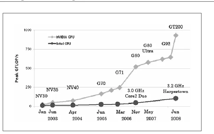
Figure 1.4: Growth trend of NVIDIA GPU vs. CPU (Source: NVIDIA).

kernel functionsare assembled in a single program [1]. The host program or so-calledmain programis executed on the CPU. In contrast, thekernel functionsare executed in a massively parallel fashion on hundreds of processors on the GPU. Analogous techniques are also offered by ATI using the brand names Close-to-Metal, Stream SDK, and Brook-GP.

(28)

10 1. Preliminaries

(29)

1.6 Outline of the Thesis 11

1.6 Outline of the Thesis

In this thesis, we aim at discovering novel data mining algorithms for mining dif-ferent kinds of data structures. In addition, we focus on boosting opportunities for computationally intensive steps of the data mining process. The detailed outline is given in the following.

In Chapter 1, we give the reader a short introduction to the broader context of this thesis. In Chapter 2, we provide a brief overview of traditional data mining algo-rithms on structured data and present a rather general survey on advanced cluster-ing methods. In addition, we introduce the broad related work on techniques for boosting the data mining process by an intelligent adoption of Graphics Process-ing Units (GPUs).

(30)

12 1. Preliminaries

Chapter 7 presents our work on data mining using GPUs. Section 7.1 explains the graphics hardware and the CUDA programming model underlying our pro-cedures. In Section 7.2, we develop a multi-dimensional index structure for si-milarity queries on the GPU that can be used for further accelerations of the data mining process. Section 7.3 presents non-indexed as well as indexed algorithms to perform the similarity join on graphics hardware. Section 7.4 and Section 7.5 are dedicated to GPU-capable algorithms for density-based and partitioning clus-tering. The contributions on data mining using GPUs have already been published by the author in two publications [15, 14].

(31)

Chapter 2 Related Work

To survey the large work on performing data mining of structured data, we mainly focus on well-known clustering techniques for hierarchical data in Section 2.1 as well as for mixed type attributes data in Section 2.2. In Section 2.3, we describe some ideas of how to enhance the effectiveness of many data mining concepts by information theory. In the field of graph mining, we present different algorithms for finding interesting patterns, i.e. frequent subgraphs in one large network or in a given set of networks (cf. Section 2.4). Finally, we conclude the related research on acceleration opportunities for the data mining process by the use of graphics processors.

2.1 Hierarchical Clustering

(32)

14 2. Related Work

Figure 2.1: The hierarchical structure, present in the dataset on the left side, is visualized by the dendrogram on the right side.

• The root of the dendrogram represents the whole datasetDS.

• Each leaf of the dendrogram corresponds to one data object ofDS.

• The internal nodes of the dendrogram are defined as the union of their chil-dren, i.e., each node represents a cluster containing all objects in the corre-sponding subtree.

• Each level of the dendrogram represents a partition of the dataset into dis-tinct clusters.

(33)

2.1 Hierarchical Clustering 15

Most hierarchical methods belong to this category. They differ only in their defi-nition of between-cluster similarity.

Divisive hierarchical clustering works in the opposite way - it starts with all data objects in one root cluster and subdivides them into smaller clusters until each cluster consists of only one single data object. Divisive methods are not generally available, and have been rarely applied. The reason for this is mainly computational - divisive clustering is more computationally expensive when it comes to making decisions in dividing a cluster in two clusters given all possible choices. While in agglomerative procedures in one step two out of maximum n elements have to be chosen for merging, in divisive procedures fundamentally all subsets have to be analyzed so that divisive procedures have an algorithmic complexity ofO(2n).

2.1.1 Agglomerative Hierarchical Clustering

Given a datasetDS ofn objects, the basic process of agglomerative hierarchical clustering is defined as follows:

1. Place each data object xi ∈ DS (i = 1, . . . n) in one single cluster Ci.

Create the list of initial clustersC=C1, . . . , Cn, which will build the leaves

of the resulting dendrogram.

2. Find the two clustersCi, Cj ∈Cwith the minimum distance to each other.

3. Merge the clustersCi andCj to create a new internal nodeCij which will

be the parent ofCi andCj in the resulting dendrogram. RemoveCi andCj

fromC.

4. Repeat step (2) and (3) until the total number of clusters inCbecomes one.

(34)

16 2. Related Work

together, a linkage rule is needed to determine the actual distance between two clusters. There are numerous linkage rules that have been proposed. In the fol-lowing, some of the most commonly used are presented.

2.1.2 Linkage methods

LetDS be a dataset,distdenotes the distance function between the data objects ofDS, and letCi andCj be two disjunct clusters consisting of objects ofDS, i.e.

Ci, Cj ⊆ DS and Ci ∩Cj = ∅. In the following, some of the most commonly

used linkage rules to determine the distance between two clusters are described.

Single Link

One of the most widespread approaches to agglomerative hierarchical clustering is Single Link [72]. Single Link defines the distance distSL between any two

clustersCi and Cj as the minimum distance between them, i.e. as the distance

between the two closest objects:

distSL(Ci, Cj) = min xi∈Ci,xj∈Cj

{dist(xi, xj)}.

Using the Single Link method often causes thechaining phenomenon, also called

Single Link effect, which is a direct consequence of the Single Link approach tending to build a chain of objects that connects two clusters.

Complete Link

The Complete Link method [25] is the opposite of Single Link. Complete Link defines the distancedistCL between any two clustersCi andCj as the maximum

distance between them:

distCL(Ci, Cj) = max xi∈Ci,xj∈Cj

(35)

This method should not be used if there is a lot of noise expected to be present in the dataset. It also produces very compact clusters. This method is useful if one is expecting objects of the same cluster to be far apart in multi-dimensional space. In other words, outliers are given more weight in the cluster decision.

Average Link

Average Link [98] calculates the mean distance between all possible pairs of ob-jects belonging to the two clusters Ci andCj. Hence, it is computationally more

expensive to compute the distancedistAV Gthan the aforementioned methods:

distAV G(Ci, Cj) =

1

|Ci| · |Cj|

X

xi∈Ci,xj∈Cj

{dist(xi, xj)}.

Average Link is sometimes also referred to as UPGMA (Unweighted Pair-Group Method using Arithmetic averages). There are several other variations of this method, e.g. Weighted Pair-Group Average, Unweighted Pair-Group Centroid, Weighted Pair-Group Centroid, but one should understand that it is a tradeoff between Single Link and Complete Link.

2.1.3 Density-based Hierarchical Clustering

(36)

18 2. Related Work

ε₁

ε₂ B

B

A₁ A₂ A

Figure 2.2: The reachability plot computed by OPTICS for a given sample 2-dimensional dataset.

sample 2-dimensional dataset. Valleys in this plot indicate clusters: objects hav-ing a small reachability value are closer and thus more similar to their predecessor objects than objects having a higher reachability value. The reachability plot gen-erated by OPTICS can be cut at any level0 parallel to the x-axis. It represents the partitioning according to the density threshold0. A consecutive subsequence of objects having a smaller reachability value than0 belongs to the same cluster then. Referring to the given example in Figure 2.2, a cut at the level1 results in

two clustersAandB. Compared to this clustering, a cut at level2 would yield

three clusters. The clusterAis split into two smaller clusters denoted byA1 and

A2 and clusterB decreased its size. This illustrates, how the hierarchical cluster

structure of a dataset is revealed at a glance and can be easily explored by visual inspection.

(37)

2.1.4 Model-based Hierarchical Clustering

For many applications and further data mining steps, it is essential to have a model of the data. Hence, clustering with PDFs, which goes back to the popular EM al-gorithm [27], is a widespread approach for performing clustering. EM is a gener-alization of thek-means algorithm, a partitioning clustering algorithm for numeri-cal data (cf. Section 2.2.1). After a suitable initialization, EM iteratively optimizes a mixture model ofk Gaussian distributions until no further significant improve-ment of the log-likelihood of the data can be achieved. In detail, we generate a dataset that consists of first picking a centroid at random and then adding some noise. If the noise is normally distributed, this procedure will result in clusters of spherical shape. Model-based clustering assumes that the data were generated by a model and tries to recover the original model from the data. More precisely, the data has been generated from a finite mixture of k distributions, but that the cluster membership of each data point is not observed. In EM, the log-likelihood is used to calculate the model parametersθ:

L(θ) = log

n

Y

i=1

P(xi|θ) = n

X

i=1

logP(xi|θ)

Model-based clustering aims for determine the parameter θˆthat maximizes the log-likelihood:

L(ˆθ) = max

θ L(θ) = maxθ n

X

i=1

logP(xi|θ)

In the case ofkclusters a vector~θ ={θ1,· · · , θk}has to be optimized:

L(~θ) =

n

X

i=1

logP(xi|~θ) = n X i=1 k X j=1

logWj+ logP(xi|θj)

,

whereWj is the weight of the cluster that represents the number of objects

(38)

20 2. Related Work

EM can be applied to many different types of probabilistic modeling. In case the probability density function (PDF) which is associated to a cluster C is a multivariate Gaussian in ad-dimensional space which is defined by the parameters µC andΣC (whereµC = (µC,1, ..., µC,d)Tis a vector from ad-dimensional space,

called the location parameter, andΣC is ad×dcovariance matrix), the definition

ofP(x|θ)is as follows: P(x|µC,ΣC, x) =

1 p

(2π)d_{· |}_Σ C|

·e−12(x−µC)T·Σ−C1·(x−µC)_.

The EM algorithm is an iterative procedure where in each iteration step the mix-ture model of the k distributions are optimized until no further significant im-provement of the log-likelihood of the data can be achieved. Usually, a very fast convergence of EM is observed. However, the algorithm may get stuck in local maximum of the log-likelihood. Moreover, the quality of the clustering result strongly depends on an appropriate choice ofk, which is a non-trivial task in most applications.

A hierarchical extension of the EM algorithm was presented by Vasconcelos and Lippman in 1998 [97]. The efficiency of this approach is achieved by pro-gressing the data in a bottom-up fashion, i.e. the mixture components of a given level are clustered to retrieve those components of the level above. This procedure requires only knowledge of the mixture parameters, the intermediate samples do not have to be resorted. With regards to practical applications, this algorithm leads to computationally efficient methods for estimating density hierarchies capable of describing data at different resolutions.

2.2 Mixed Type Attributes Data

(39)

2.2 Mixed Type Attributes Data 21

integrative data mining algorithms have to be scalable and capable of dealing with different types of attributes. In terms of clustering, we are interested in algo-rithms which can efficiently cluster large datasets containing both numeric and categorical values because such datasets are frequently encountered in data min-ing applications. The traditional way to treat categorical attributes as numeric does not always produce meaningful results because many categorical domains are not ordered.

One simple idea for performing integrative clustering on heterogeneous data is to combinek-means based methods with thek-modes algorithm. The algorithm k-prototypes derives advantage from this combination, and is therefore one of the first approaches towards integrative clustering.

2.2.1 The

k

-means Algorithm for Clustering Numerical Data

Thek-means algorithm [72] is one of the mostly used partitioning non-hierarchical clustering approach. The procedure follows a simple and easy way to group a given datasetDSconsisting ofnnumeric objects into a certain number ofk(< n) clusters. First, k centroids are defined, one for each cluster. Then, the algorithm takes each point of DS and associates it to the nearest centroid, until no more point is pending. Afterwards, the k new centroids (the mean value µ over the coordinates of all data points belonging to the specific cluster) are recalculated, and thus, a new association has to be determined between the points of DS and the nearest new centroid. These two steps are performed until no more location changes of the centroids are observed. Finally, k-means aims at minimizing an objective function, in this case the within clusters sum of squared errors (WCSS).

W CSS =

k

X

j=1

n

X

i=1

(dist(xi,j, µj))2,

wheredist(xi,j, µj)is a chosen distance function between a data pointxi,jand the

centroidµj of clusterCj, is an indicator of the distance of thendata points from

(40)

22 2. Related Work

The main advantage ofk-means is its efficiency. It can be proven that convergence is reached inO(n)iterations. However, this method has four major drawbacks: First, the number of clustersk has to be specified in advance, second, the clus-ter compactness measure WCSS and thus the clusclus-tering result is very sensitive to noise and outliers. In addition,k-means implicitly assumes a Gaussian data dis-tribution, and is thus restricted to detect spherically compact clusters. The major drawback lies in its limited practicability to numeric data.

2.2.2 Conceptual Clustering Algorithms for Categorical Data

In principle the formulation of the WCSS in Section 2.2.1 is also valid for cate-gorical and mixed type objects. The reason why thek-means algorithm cannot cluster categorical objects is that the calculation of the mean value is not defined for categorical data. These limitations can be removed by the following modifica-tions:

• Use a simple matching distance function for categorical objects.

• Replace means as cluster representatives by modes.

• Use a frequency-based method to find the modes.

A Distance Function for Categorical Objects

Letx,ybe two categorical objects described bymcategorical attributes. The dis-tance function between these two objects can be defined by the total mismatches of the corresponding attribute categories of the two objects. The smaller the num-ber of mismatches is, the more similarxandy. This measure is often referred to assimple matching[56]. Formally this distance function is defined as follows:

distSimple(x, y) = m

X

i=1

δ(xi, yi), where δ(xi, yi) =

  

0, ifxi =yi,

(41)

2.2 Mixed Type Attributes Data 23

Modes as Cluster Representatives

Consider a set of n categorical objects X described by categorical attributes, A1, A2,· · · , Am. The mode of this set is an arrayq = [q1, q2,· · · qm] of length

mthat minimizes the following formula:

D(X, q) =

n

X

i=1

distSimple(Xi, q)

Calculation of the Modes

Let nck,i be the number of objects having the k-th category ck,i in attribute Ai,

and let p(Ai = ck,i|X) be the relative frequency of categoryck,iin X. Then the

functionD(X, q)is minimized if and only ifp(Ai =qi|X) ≥p(Ai =ck,i|X)for

qi 6=ck,ifor alli∈ {1,· · · , m}[48].

This theorem defines a way to find the modeqfrom a given set of categorical objects X, and therefore it is important because it allows thek-means paradigm to be used to cluster categorical data.

The Algorithmk-modes

Conceptual clustering algorithms, like k-modes [49] implement the idea of clus-tering categorical data by using distSimple as distance function and by means of

the aforementioned modifications of k-means clustering. The procedure of the algorithmk-modes can be summarized as follows:

1. Selectkinitial modes, one for each cluster.

2. Allocate an object to the cluster whose mode is the nearest to it according to the distance functiondistSimple; update the mode of the cluster after each

allocation according to the theorem presented in Section 2.2.2.

(42)

24 2. Related Work

belongs to another cluster rather than its current one, reallocate the object to that cluster and update the modes of both clusters.

4. Repeat step (3) until no object has changed clusters after a full cycle test of the whole dataset.

Like thek-means algorithm, thek-modes algorithm also produces locally optimal solutions that are dependent on the initial modes and the order of objects in the dataset. Its efficiency relies on good search strategies. For data mining problems, which often involve many concepts and very large object spaces, the concepts based search methods can become a potential handicap for these algorithms to deal with extremely large datasets.

2.2.3 The

k

-prototypes Algorithm for Integrative Clustering

One of the first algorithms for integrative clustering isk-prototypes [47]. The dis-tance between two mixed type objectsxandy, which are described bymattributes An

1, An2,· · · , Anp, Apc+1, Acp+2,· · · , Acmis measured by the following formula:

distM ixed =

p

X

i=1

(xi−yi)2+γ m

X

i=p+1

δ(xi, yi).

The first term is the squared Euclidean distance measure on the p numeric at-tributes An

i and the second term is the simple matching distance function on the

m−pcategorical attributesAc

i. The weightγis used to avoid favoring either type

of attribute. The influence of this parameter in the clustering process is discussed in the publication by Huang [47].

2.3 Information Theory in the Field of Clustering

(43)

2.3 Information Theory in the Field of Clustering 25

on parameter-free partitioning clustering and are based on the Akaike Information Criterion (AIC), the Bayesian Information Criterion (BIC) and Minimum Descrip-tion Length (MDL) [40]. For these methods, the data itself is the only source of knowledge. Information theoretic arguments are applied for model selection dur-ing clusterdur-ing, and these approaches involve a lossless compression of the data.

The work of Still and Bialek [91] provides important theoretical background by using information-theoretic arguments to relate the maximum number of clusters that can be detected by partitioning clustering with the size of the dataset. The algorithm X-Means [81] combines thek-means paradigm with BIC for parameter-free clustering. X-Means involves an efficient top-down splitting algorithm where intermediate results are obtained by bisecting k-means and are evaluated with BIC. However, only spherically Gaussian clusters can be detected. The algorithm G-means (Gaussian means) introduced in [43] has been designed for parameter-free correlation clustering. G-means follows a similar algorithmic paradigm as X-Means with top-down splitting and the application of bisecting k-means upon each split. However, the criterion to decide whether a cluster should be split up into two is based on a statistical test for Gaussianity. Splitting continues until the clusters are Gaussian, which implies of course, that non-Gaussian clusters can still not be detected. The algorithm PG-means (Projected Gaussian means) by Feng and Hamerly [33] is similar to G-means but learns models with increasing k with the EM algorithm. In each iteration, various 1-dimensional projections of the data and the model are tested for Gaussianity. Experiments demonstrate that PG-means is less prone to over-fitting than G-means.

(44)

26 2. Related Work

pdf_{Lapl(μ=3.5 σ=1)}(x)

5 % 4.3 Bit

pdf_{Gauss(μ=3.5 σ=1)}(y) x

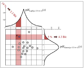
Figure 2.3: Coding scheme for cluster objects of the RIC algorithm. In addition to the data, type and parameters of the PDF need to be coded for each cluster.

clustering. It is based on MDL and introduces a coding scheme especially suit-able for clustering together with algorithms for purifying the initial clusters from noise. In a first step, RIC removes noise objects from the initial clusters, and then merges clusters if this allows for more effective data compression. The algorithm operates with arbitrary data distributions, taken from a fixed set of PDFs.

(45)

2.4 Graph-structured Data 27

a more extreme example) are assigned longer patterns. Provided that a coordi-nate is really distributed according to the assumed distribution function, Huffman codes optimize the overall compression of the dataset. Huffman codes associate a bit string of length l = log2(1/p(pi))to each coordinate pi, wherep(pi)is the

probability of the (discretized) coordinate value.

The algorithm OCI (Outlier-robust Clustering using Independent Components) [11] provides parameter-free clustering of noisy data and allows detecting non-Gaussian clusters with non-orthogonal major directions. Technically this is achieved by defining a very general cluster notion based on the Exponential Power Distribution (EPD) and by integrating Independent Component Analysis (ICA) into clustering. The EPD includes a wide range of symmetric distribution functions, e.g. Gaus-sian, Laplacian and uniform distributions and an infinite number of hybrid types in between by an additional shape parameter. Beyond correlations detected by Prin-cipal Component Analysis (PCA), which correspond to correlation clusters with orthogonal major directions, ICA allows to detect general statistical dependencies in the data.

2.4 Graph-structured Data

In this section, we review the previous work on finding patterns in graph data and focus on three problems. First, frequent subgraphs across a dataset of graphs. Sec-ond, frequent subgraphs within one single large graph. Third, frequent subgraphs in dynamic graph data.

2.4.1 Graph Dataset Mining

(46)

28 2. Related Work

X

Y

Z

X

b

a

_b

v

₀

v

₁

v

₂

v

₃

X

Y

Z

X

b

a

_b

v

₀

v

₁

X

Y

Z

X

b

a

_b

v

₀

v

₁

backward extension forward extension

v

₂

v

₃

v

₂

v

₃

Figure 2.4: Illustration of the rightmost extension used in gSpan.

representation of subgraphs in order to reduce runtime costs for subgraph isomor-phism checking.

Similar to AGM, FSG (Frequent SubGraph Discovery) [61] uses a canonical labeling based on the adjacency matrix. Canonical labeling, candidate generation and evaluation are sped up in FSG using graph invariants and the Transaction ID principle, which stores the ID of transactions a subgraph appeared in. This speed-up is paid for by reducing the class of subgraphs discovered to connected subgraphs, i.e. subgraphs where a path exists between all pairs of nodes.

The most well-known member of the class of pattern-growth algorithms, gSpan (graph-based Substructure pattern mining) [107], discovers frequent substructures efficiently without candidate generation. It is built on depth first search (DFS) tree. Given a graphSwith nodesN and edgesE, and a DFS treeT R, we call the start-ing node inT R,v0, the root, and the last visited node,vn, therightmost node. The

straight path fromv0tovnis called therightmost path. Figure 2.4 shows an

exam-ple. The red edges form a DFS tree. The nodes are discovered in the orderv0,v1,

v2,v3. The nodev3 is the rightmost node. The rightmost path isv0 →v1 →v3.

(47)

2.4 Graph-structured Data 29

rightmost path (forward extension). If we want to extend the graph in Figure 2.4, the backward extension candidate can be (v3, v0). The forward extension

candi-dates can be edges extending fromv3, v1 or v0 with a new node inserted. Since

there could be multiple DFS trees for one graph, gSpan establishes a set of rules to select one of them as representative so that the backward and forward extensions will only take place on one DFS tree.

Overall, new edges are only added to the nodes along the rightmost path. With this restricted extension, gSpan reduces the generation of the same graphs, and defines a canonical form of S. However, it still guarantees the completeness of enumerating all frequent subgraphs.

2.4.2 Large Graph Mining

(48)

30 2. Related Work

discover multiple patterns and to find longer patterns in fewer iterations. Finally, GREW uses a representation of the rewritten graph that retains all the information present in the original graph, and thus it precisely identifies whether or not there is an embedding of a particular subgraph. This result guarantees a lower bound on the frequency of each discovered pattern. SUBDUE tries to minimize the min-imum description length (MDL) of a graph by compressing frequent subgraphs. Frequent subgraphs are replaced by one single node and the MDL of the remain-ing graph is then determined. Those subgraphs whose compression minimizes the MDL are considered frequent patterns in the input graph. The candidate graphs are generated starting from single nodes to subgraphs with several nodes, using a computationally constrained beam search.

Similarly, vSIGRAM and hSIGRAM [62] find subgraphs that are frequently embedded within a large sparse graph, using “horizontal” breadth-first search and “vertical” depth-first search, respectively. They employ efficient algorithms for candidate generation and candidate evaluation that exploit the sparseness of the graph.

While most of the techniques mentioned before often use some sort of heuris-tic search strategy that repeatedly compresses the graph to find frequent sub-graphs, methods based on sampling subgraphs to estimate their frequency are pre-dominant in application domains, like bioinformatics [55, 102]. Another strategy is to exhaustively enumerate all subgraphs. This has the advantage that one can then compute exact rather than approximate frequencies, but for large graphs, it is only feasible for subgraphs with a limited numberkof nodes, typicallyk ∈ {3,4}.

2.4.3 Dynamic Graph Mining

(49)

2.5 Boosting Data Mining 31

dynamic graphs so far.

2.5 Boosting Data Mining

In this section, we survey the related research in general purpose computations using Graphics Processing Units (GPUs) with particular focus on database man-agement and data mining.

Figure 2.5: The NVIDIA GeForce 8800 GTX graphics processor (Source: NVIDIA).

2.5.1 General Processing-Graphics Processing Units

(50)

32 2. Related Work

and DNA databases, running on GPU and implemented in the CUDA program-ming environment. This algorithm launches a great number of parallel threads simultaneously to fully exploit the huge computational power of the GPU. It pur-sues the strategy that each GPU thread computes the whole alignment of the query sequence with one database sequence. All threads are grouped in a grid of blocks when running on the graphics card. In order to make the most efficient use of the GPU resources the computing time of all threads in the same grid must be as near as possible. For this reason, the sequences of the database are pre-ordered w.r.t. their length. Hence, all adjacent threads align the query sequence with two database queries having the nearest possible sizes.

Another widespread application area that uses the processing power of the GPU is mechanical simulation. One example is the work by Tascoraet al.[94], that presents a novel method for solving large cone complementarity problems by means of a fixed-point iteration algorithm, in the context of simulating the fric-tional contact dynamics of large systems of rigid bodies. The proposed algorithm is well suited for running on parallel platforms that support the single instruction multiple data (SIMD) computational paradigm, which is ideally suited for han-dling problems with contacts in excess of hundreds of thousand.

(51)

2.5 Boosting Data Mining 33

2.5.2 Database Management Using GPUs

Some research papers propose techniques to speed up relational database oper-ations on GPU. Two recent papers [67, 16] address the topic of similarity join in feature space which determines all pairs of objects from two different sets R and S fulfilling a certain join predicate. The most common join predicate is the SJ-join which determines all pairs of objects having a distance of less than a

predefined threshold SJ. The authors of [67] propose an algorithm based on the

concept of space filling curves, e.g. thez-order, for pruning the search space, run-ning on an NVIDIA GeForce 8800 GTX using the CUDA toolkit. The z-order of a set of objects can be determined very efficiently on GPU by highly paral-lelized sorting. Their algorithm operates on a set ofz-lists of different granularity for efficient pruning. However, since all dimensions are treated equally, perfor-mance degrades in higher dimensions. An approach that overcomes that kind of problem is presented in [16]. Here, the authors parallelize the baseline technique underlying any join operation with an arbitrary join predicate, namely the nested loop join (NLJ), a powerful database primitive that can be used to support many applications including data mining.

(52)

34 2. Related Work

2.5.3 Data Mining Using GPUs

Finally, we survey some recent approaches for data mining using the GPU. In [20] a parallelized clustering approach for graphics hardware is presented. This algo-rithm extends the basic idea of k-means clustering by calculating the distances from a single input centroid to all objects at one time that can be done simulta-neously in hardware. Thus the authors are able to exploit the high computational power and pipeline of GPUs, especially for core operations, like distance com-putations and comparisons. An additional efficient method that is designed to execute clustering on data streams confirms a wide practical field of clustering on GPU.

The algorithm k-means was also parallelized by Shalomet al. [87]. In their implementation multi-pass rendering and multi shader program constants are used. This is done by minimizing the use of GPU shader constants, which leads to a significant improvement of the performance as well as to a reduction of the data transactions between the CPU and the GPU. Handling data transfers between the necessary textures within the GPU is much more efficient than using shader constants. This is mainly due to the high memory bandwidth available in the GPU pipeline. Since all the steps of thek-means algorithm are able to be imple-mented in the GPU, the transferring of data back to the CPU during the iterations is avoided. The programmable capabilities of the GPU have been thus exploited to efficiently implementk-means clustering in the GPU.

(53)

Chapter 3 Hierarchical Data Mining

Since dendrograms and similar hierarchical representations provide extremely useful insights into the structure of a dataset, hierarchical clustering has become very popular in various scientific disciplines, such as molecular biology, medicine, or economy. However, well-known hierarchical clustering algorithms often either fail to detect the true clusters that are present in a dataset, or they identify invalid clusters, which are not existing in the dataset. These problems are particularly dominant in the presence of noise and outliers.

(54)

36 3. Hierarchical Data Mining

3.1 ITCH: An EM-based Hierarchical Clustering

Al-gorithm

Many hierarchical clustering problems result in the questions “How can we de-cide if a given representation is really natural, valid, and therefore meaningful?” and “How can we enforce a hierarchical clustering algorithm to identify only the meaningful cluster structure?”

Information Theory for Clustering. We give the answer to these questions by relating the hierarchical clustering problem to that of information theory and data compression. Imagine you want to transfer the dataset via an extremely expensive and small-banded communication channel. Then you can interpret the hierarchy as a statistical model of the dataset, which defines more or less likely areas of the data space. This knowledge can be used for an efficient compression of the dataset. Following the idea of (optimal) Huffman coding, we assign few bits to points in areas of high probability and more bits to areas of low probability. The interesting observation is the following: the compression becomes the more ef-fective, the better our statistical model fits to the data. This so-called Minimum Description Length(MDL) principle has recently received increasing attention in the context of partitioning (i.e. non-hierarchical) clustering methods. Note that it can not only be used to assess and compare the quality of the clusters found by dif-ferent algorithms and/or varying parameter settings. Rather, we use this concept as an objective function to implement clustering algorithms directly using simple but efficient optimization heuristics.

We extend the idea of MDL to the hierarchical case and develophM DL for

(55)

3.1 ITCH: An EM-based Hierarchical Clustering Algorithm 37

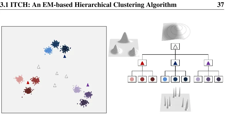
Figure 3.1: ITCH gives the hierarchical representation of a complex dataset con-sisting of three clusters, where each cluster contains three subclusters. Outliers are placed on different hierarchy levels and represented by the symbol ∆ in the corresponding color. Besides the hierarchical structure, ITCH provides a model of each cluster content in form of a Gaussian PDF.

Challenges and Contributions. With an assessment condition for cluster hier-archies, we develop a complete hierarchical clustering approach on top of the idea of hM DL. This proposed algorithm ITCH (Information-TheoreticCluster

Hierarchies) yields numerous advantages, out of which we demonstrate the fol-lowing four:

1. All single clusters as well as their hierarchical arrangement are guaranteed to bemeaningful. Nodes only are placed in the cluster hierarchy if they im-prove the data compression. This is achieved by optimizing thehM DL cri-terion. Moreover, a maximal consistency with partitioning clustering meth-ods is obtained.

(56)

3. ITCH has a consistent outlier-handling. Outliers are assigned to the root of the cluster hierarchy or to an appropriate inner node, depending on the degree of outlierness. For example, in Figures 3.1 the outlier w.r.t. the three red clusters at the bottom level is assigned to the parent cluster in the hierarchy, marked by a red triangle.

4. ITCH isfully automaticas no difficult parameter settings are necessary.

3.1.1 Information-theoretic Hierarchical Clustering

The clustering problem is highly related to that of data compression: The detected cluster structure can be interpreted as a PDF fΘ(x)where Θ = {θ1, θ2, ...} is a

set of parameters, and the PDF can be used for an efficient compression of the dataset. It is well-known that the compression by Huffman coding is optimal if the data distribution really corresponds to fΘ(x). Huffman coding represents

every pointxby a number of bits which is equal to the negative binary logarithm of the PDF:

C_data(x) =−log₂(fΘ(x)).

The better the point set corresponds tofΘ(x), the smaller the coding costsC_data(x)

(57)

the Huffman coding of Θ, and different assumptions lead to different objective functions. In case of the hierarchical cluster structure in ITCH, a very natural distribution function forΘexists: With the only exception of the root node, every node in the hierarchy has a parent node. This parent node is associated with a PDF which can naturally be used as a code book for the mean vector (and indirectly also for the variances) of the child node. The coding costs of the root node, how-ever, are not important, because every valid hierarchy has exactly one root node with a constant number of parameters, and therefore, the coding costs of the root node are always constant.

Hierarchical Cluster Structure

In this Section, we formally introduce the notion of a hierarchical cluster structure (HCS). A HCS contains clusters {A, B, ...} each of which is represented by a Gaussian distribution function. These clusters are arranged in a tree:

Definition 1 (Hierarchical Cluster Structure)

(1) AHierarchical Cluster StructureHCSis a treeT = (N,E)consisting of a set of nodes N = {A, B, ...}and a set of directed edges E = {e1, e2, ...}where

A is a parent ofB (B is a child of A) iff(A, B) ∈ E. Every node C ∈ N is associated with a weightWC and a Gaussian PDF defined by the parametersµC

andΣC such that the sum of the weights equals one:

X

C∈N

WC = 1.

(2) If a path fromAtoB exists inT (orA=B) we callAan ancestor ofB (Ba descendant ofA) and writeB vA.

(3) The levellC of a nodeCis the height of the descendant subtree. IfCis a leaf,

thenChas levellC = 0. The root has the highest level (length of the longest path

(58)

The PDF which is associated with a cluster C is a multivariate Gaussian in ad -dimensional data space which is defined by the parameters µC and ΣC (where

µC = (µC,1, ..., µC,d)T is a vector from ad-dimensional space, called the location

parameter, andΣC is ad×dcovariance matrix) by the following formula:

N(µC,ΣC, x) =

1 p

(2π)d_{· |}_Σ C|

·e−12(x−µC) T_·_Σ−1

C ·(x−µC)_.

For simplicity we restrictΣC = diag(σ2C,1, ..., σC,d2 )to be diagonal such that the

multivariate Gaussian can also be expressed by the following product:

N(µC,ΣC, x) =

Y

1≤i≤d

N(µC,i, σC,i2 , xi)

= Y

1≤i≤d

1 q

2πσ2

C,i

·e

−(xi−µi)2

2σ2 C,i _.

Since we require the sum of all weights in a hierarchical cluster structure HCS to be1, a HCS always defines a function whose integral is≤1. Therefore, the HCS can be interpreted as a complex, multimodal, and multivariate PDF, defined by the mixture of the Gaussians of the HCST = (N,E):

fT(x) = max

C∈N{WCN(µC,ΣC, x)}with

Z

Rd

fT(x)dx≤1.

If the Gaussians of the HCS do not overlap much, then the integral becomes close to 1.

The operations, described in Section 3.1.1, assign each point x ∈ DB to a cluster of the HCS T = (N,E). We distinguish between the direct and the

(59)

Level ₂

Level ₁

Level ₀

0.2 0.2

0.5 0.1 0.1

0.1 0.1

0.7

Figure 3.2: Hierarchical cut T0 _{of the HCS}_T _{at level 1. All weights are placed}

inside the corresponding nodes.

Cl(x) = arg max

C∈N {WC ·N(µC,ΣC, x)}.

As we have already stated in the introduction, one of the main motivations of our hierarchical, information-theoretic clustering method ITCH is to represent a sequence of clustering structures which range from a very coarse (unimodal) view to the data distribution to a very detailed (multimodal) one, and that all these views are meaningful and represent an individual complex PDF. The ability to cut a cluster hierarchy at a given levelLis obtained by the following definition:

Definition 2 (Hierarchical Cut) A HCST0 _{= (}_N0_,_E0₎_{is a}_{hierarchical cut}_{of a} HCST = (N,E)at levelL, if the following properties hold:

(1)N0 ₌_{_A_{∈ N |}_l

A≥L},

(2)E0 ₌_{₍_{A, B}₎_{∈ E|}_l

A> lB ≥L},

(3) For eachA ∈ N0_{the following properties hold:}

W_A0 = (

WA iflA> L

P

B∈N,BvAWB otherwise,

whereWC andWC0 is the weight of nodeCinT andT

(60)

(4) Analogously, for the direct association of points to clusters the following prop-erty holds: Letxbe associated with ClusterB inT, i.e.Cl(x) =B. Then inT0_,

xis associated with:

Cl0(x) = (

B iflB ≥L

A|B vA∧lA=L otherwise.

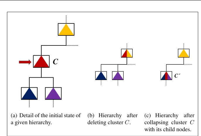
Here, the weights of the pruned nodes are automatically added to the leaf nodes of the new cluster structure, which used to be the ancestors of the pruned nodes. Therefore, the sum of all weights is maintained (and still equals 1), and the ob-tained tree is again a HCS according to Definition 1. The same holds for the point-to-cluster assignments. Figure 3.2 presents an illustrative example of the hierarchical cut.

Generalization of the MDL Principle

Now we explain how the MDL principle can be generalized for hierarchical clus-tering and develop the new objective functionhM DL. Following the traditional MDL principle, we compress the data points according to their negative log like-lihood corresponding to the PDF which is given by the cluster hierarchy. In ad-dition, we penalize the model complexity by adding the code length of the HCS parameters to the negative log likelihood of the data. The better the PDFs of child nodes fit into the PDFs of the parent, the less the coding costs will be. Therefore, the overall coding costs corresponds to the natural, intuitive notion of a good hier-archical representation of data by distribution functions. The discrete assignment of points to clusters allows us to determine the coding costs of the points cluster-wise and dimensioncluster-wise, as explained in the following: The coding costs of the points associated with the clustersC ∈ N of the HCST = (N,E)corresponds to:

C_data =−log₂ Y

x∈DB

max

C∈N

WC

Y

1≤j≤d

N(µC,j, σC,j2 , xj)

(61)

Since every point x is associated with that cluster C in the hierarchy which has maximum probability density, we can rearrange the terms of the above formula and combine the costs of all points that are in the same cluster:

= −X

x∈DB

log₂

WCl(x)

Y

1≤j≤d

N(µCl(x),j, σCl2 (x),j, xj)

= −

X

C∈N

nWClog2WC

+

X

x∈DB;

X

1≤j≤d

log₂N(µCl(x),j, σ2Cl(x),j, xj)

= −X

C∈N

nWClog2WC+

X

x∈C;

X

1≤j≤d

log₂N(µC,j, σC,j2 , xj)

,

where WCl(x) is the weight of the cluster in the hierarchy which has maximum

probability density for the point x. The ability to model the coding costs of each cluster separately allows us now, to focus on a single cluster, and even on a single dimension of a single cluster. A common interpretation of the term

−nWClog2WC, which actually comes from the weight a single Gaussian

con-tributes to the GMM, is a Huffman coding of the cluster ID. We assume that every point carries the information which cluster it belongs to, and a cluster with many points gets a shortly coded cluster ID. These costs are referred to theID cost of a clusterC.

Consider two clusters, A and B, where B v A. We now want to derive the coding scheme for the cluster B and its associated points. Several points are associated withB, where the overall weight of assignment sums up toWB. When

coding the parameters of the associated PDF of B, i.e. µB, and σB, we have

to consider two aspects: (1) The precision both parameters should be coded to minimize the overall description length depends on WB, as well as on σB. For

instance, if only few points are associated with clusterB and/or the varianceσB

is very large, then it is not necessary to know the position of µB very precisely

(62)

m_B

mB ~

(a) Exact coding of the location parameter

µB. µeB of the coding Gaussian function fits

exactly toµBof the data distribution.

m_B

mB ~

(b) Inexact coding of the location parameter

µBby some regular quantization grid.

m_B

(c) Different Gaussians w.r.t. different grid positions.

(d) Complete interval of all possible values

for the recovered location parameterµBw.r.t.

to the PDF of the predecessor clusterA.

(63)

can assign fewer bits. Basically, model selection criteria, such as the Bayesian Information Criterion (BIC) or the Aikake Information Criterion (AIC) already address the first aspect, but not the hierarchical aspect. To make this thesis self contained, we consider both aspects. In contrast to BIC, which uses the natural logarithm, we use the binary logarithm to represent the code length in bits. For simplicity, we assume that our PDF is univariate and the only parameter is its mean value µB. We neglectσB by assuming e.g. some fixed value for all clusters. We

drop these assumptions at the end of this section. When the true PDF of clusterB is coded inexactly by some parameterµ_eB, the coding costs for each pointx(which

truly belongs to the distributionN(µB, σB2, x)) inB is increased compared to the

exact coding ofµB, which would result incex bits per point:

c_ex =

Z +∞

−∞

−log₂(N(µB, σB2, x))·N(µB, σ2B, x) dx= log2(σB

√

2π·e). Ifµ_eB instead ofµBis applied for compression, we obtain:

c(µ_eB, µB) =

Z +∞ −∞

−log₂(N(_eµB, σB2, x))·N(µB, σB2, x)dx.

The difference is visualized in Figure 3.3(a) and 3.3(b) respectively: In 3.3(a)µ_eB

of the coding PDF, depicted by the Gaussian function, fits exactly toµBof the data

distribution, represented by the histogram. This causes minimum code lengths for the compressed points but also a considerable effort for the coding of µB. In

Figure 3.3(b) µB is coded by some regular quantization grid. Thereby, the costs

for the cluster points slightly increase, but the costs for the location parameter decreases. The difference betweenµ_eBandµBdepends on the bit resolution and on

the position of the quantization grid. One example is depicted in Figure 3.3(b) by five vertical lines, the Gaussian curve is centered by the vertical line closest toµB.

We derive lower and upper limits of_eµB ∈[µB−1/2b...µB+1/2b]from the number

Wackersreuther, Bianca (2011): Efficient Knowledge Extraction from Structured Data. Dissertation, LMU München: Fakultät für Mathematik, Informatik und Statistik

Efficient Knowledge Extraction

from Structured Data

Bianca Wackersreuther

Efficient Knowledge Extraction

from Structured Data

Bianca Wackersreuther

Dissertation

an der Fakult¨at f¨ur Mathematik, Informatik und Statistik

der Ludwig–Maximilians–Universit¨at

M¨unchen

vorgelegt von

Bianca Wackersreuther

aus F¨ussen

Erstgutachter: Prof. Dr. Christian B¨ohm

Zweitgutachter: Prof. Dr. Thomas Seidl

Contents

Acknowledgments

Abstract

Zusammenfassung

Chapter 1

Preliminaries

1.1

The Classic Definition of KDD

1.2

Data Mining: The Core Step of Knowledge

Ex-traction

1.3

Clustering: One of the Major Data Mining Tasks

1.4

Information Theory for Clustering

1.5

Boosting the Data Mining Process

1.6

Outline of the Thesis

Chapter 2

Related Work

2.1

Hierarchical Clustering

2.1.1

Agglomerative Hierarchical Clustering

2.1.2

Linkage methods

2.1.3

Density-based Hierarchical Clustering

2.1.4

Model-based Hierarchical Clustering

2.2

Mixed Type Attributes Data

2.2.1

The

k

-means Algorithm for Clustering Numerical Data

2.2.2

Conceptual Clustering Algorithms for Categorical Data

2.2.3

The

k

-prototypes Algorithm for Integrative Clustering

2.3

Information Theory in the Field of Clustering

2.4

Graph-structured Data

2.4.1

Graph Dataset Mining

X

Y

Z

X

b

a

a

b

v

v

v

v

X

Y

Z

_b

_b

_b