A Cost-Effective Random Testing Method for
Programs with Non-Numeric Inputs
Arlinta C. Barus, Tsong Yueh Chen,
Member, IEEE
, Fei-Ching Kuo,
Member, IEEE
,
Huai Liu,
Member, IEEE
, Robert Merkel, and Gregg Rothermel,
Member, IEEE Computer Society
Abstract—Random testing (RT) has been widely used in the testing of various software and hardware systems. Adaptive random testing (ART) is a family of random testing techniques that aim to enhance the failure-detection effectiveness of RT by spreading random test cases evenly throughout the input domain. ART has been empirically shown to be effective on software with numeric inputs. However, there are two aspects of ART that need to be addressed to render its adoption more widespread - applicability to programs with non-numeric inputs, and the high computation overhead of many ART algorithms. We present a linear-order ART algorithm for software with non-numeric inputs. The key requirement for using ART with non-numeric inputs is an appropriate “distance” measure. We use the concepts of categories and choices from category-partition testing to formulate such a measure. We investigate the failure-detection effectiveness of our technique by performing an empirical study on 14 object programs, using two standard metrics - F-measure and P-measure. Our ART algorithm statistically significantly outperforms RT on 10 of the 14 programs studied, and exhibits performance similar to RT on three of the four remaining programs. The selection overhead of our ART algorithm is close to that of RT.
Index Terms—Random testing, adaptive random testing, category-partition method.
F
1
I
NTRODUCTIONR
ANDOMTesting (RT) [1] — that is, testing software by randomly generating inputs — is a standard testing approach. RT is also a mainstream approach for reliability estimation; for example, RT can help calculate thefailure rate, which refers to the probability of an input causing failure of the software under test. Arcuri et al. [5, pg. 258] observe that RT is “one of the most used automated testing techniques in practice”. RT has been widely applied to the testing of various systems [4], [17]. Considerable research has also been conducted to propose methodologies for generating random test cases [15], [30].Adaptive Random Testing (ART) [9] is a class of ran-dom testing techniques designed to improve the failure-detection effectiveness of RT by increasing the diversity across a program’s input domain of the test cases executed. The Fixed-Size Candidate Set ART technique (FSCS-ART), was the first ART technique, and is also the most widely studied. To generate an additional test case using FSCS-ART, a number of candidate test cases are randomly generated. The candidate that is the most “distant” from previously
This research was supported by the Air Force Office of Scientific Research through award FA9550-10-1-0406 to University of Nebraska - Lincoln. • A. C. Barus is with the Institut Teknologi Del, Kab Toba Samosir 22381,
Sumatera Utara, Indonesia. E-mail: [email protected]
• T. Y. Chen and F.-C. Kuo are with Swinburne University of Technology, Hawthorn 3122 VIC, Australia. E-mail:{tychen, dkuo}@swin.edu.au • H. Liu (corresponding author) is with Australia-India Research Centre for
Automation Software Engineering, RMIT University, Melbourne 3001 VIC, Australia. E-mail: [email protected]
• R. Merkel is with Monash University, Clayton 3800 VIC, Australia. E-mail: [email protected]
• G. Rothermel is with the Department of Computer Science and Engi-neering, University of Nebraska - Lincoln, Lincoln Nebraska 68588-0115, USA. E-mail: [email protected]
executed test cases, according to a criterion known as the max-min criterion, is selected as the next test case. The Cartesian distancemeasure is used to determine the distance between numeric inputs.
Various studies using programs with numeric inputs [9], [21] have shown that ART requires substantially fewer test cases than RT to reveal failures. However, as Ciupa et al. [11] observe, test case selection overhead can result in FSCS-ART having poorer overall cost-effectiveness than RT. The reduction in test cases required to reveal failures was, in their experiments, outweighed by selection overhead. Ar-curi and Briand [3] argue that the high selection overhead of FSCS-ART renders it unsuitable for practical use. They also observe that the effectiveness of FSCS-ART on programs with very low failure rates has not been studied – a fact that, itself, can be attributed to high selection overhead. A number of techniques, such as mirroring [8] and forget-ting [6], were proposed to reduce the overhead of various ART algorithms. More recently, Shahbazi et al. [25] proposed a new ART approach, Random Border Centroidal Voronoi Tessellations (RBCVT), which takes advantage of the proper-ties of the Voronoi tessellation to achieve test case diversity. The authors developed a novel algorithm (RBCVT-Fast) that has an O(n) selection overhead (that is, the process of generatingntest cases takesO(n)time). However, RBCVT-Fast, as presented, is only directly applicable to simple input domains representable as ad-dimensional real space.
effectiveness of this ART algorithm on 14 object programs that have non-trivial input formats, using two standard effectiveness metrics, the F-measure andP-measure, as well as test case generation time.
The remainder of this article is organized as follows. Section 2 provides essential background on ART, categories and choices. Section 3 describes the theoretical framework for applying ART to non-numeric software, and our linear-order ART algorithm. Section 4 presents our empirical study, including details on the study setup. Section 5 presents our experiment results, including quantitative statistical analy-sis of those results. Section 6 presents further interpretation and discussion of the results. Section 7 discusses related work. Some concluding thoughts, including recommenda-tions for future study, are offered in Section 8.
2
P
RELIMINARIES ANDB
ACKGROUND 2.1 ARTChen et al. [9] proposed ART as an enhancement to RT. Their approach was based on the intuition of “even spread”. A number of studies [2], [27] have found evidence that faults tend to cause erroneous behavior to occur in contiguous regions of the input domain. Thus, Chen et al. [9] argued that two test cases whose inputs were “close” to each other in the input domain were more likely to have similar execution behaviors than two test cases that were more “widely separated”. Hence, they reasoned that a method that spreads test cases more evenly would identify failures using fewer test cases.
To implement this idea, Chen et al. [9] introduced a distance-based ART algorithm, also known as Fixed-Size Candidate Set ART (FSCS-ART). In FSCS-ART, two sets of test cases are considered: theexecuted set,E, which records those test cases that have already been executed, and the candidate set. To select a new test case, a set of k candi-dates (c1, c2, . . . , ck) is first “generated randomly” as the candidate set. From these, the best candidateco is selected according to a criterion, and testing is conducted with co, which is then added to E. Testing continues until a pre-specified stopping criterion is met, such as the detection of failures, the execution of the required number of test cases.
The original FSCS-ART used themax-min criterion. For each candidateci, the Cartesian distance to each member of Eis calculated, and the smallest distance forci is recorded as di. The candidateco with the largestdi is selected (i.e., do ≥di∀i,1 ≤i ≤k). An alternative selection criterion is themax-sum criterion. In this case, for each candidate, the sumof the distances to each member ofEis calculated, and the candidate for which this sum is the largest is chosen.
ART algorithms may consider the entire set of previ-ously executed test cases when selecting the best candidate. However, as Chan et al. [6] show, it is possible to greatly reduce the selection overhead of ART techniques, while retaining much or all of their failure-revealing effectiveness, by evaluating only a subset of E when selecting the best candidate. They call this techniqueforgetting.
2.2 Categories and choices
To test software with non-numeric input formats using FSCS-ART, two things are required:
• A method for randomly sampling inputs from the software’s input domain.
• A way of measuring the “distance” between ele-ments of the software’s input domain.
The first requirement is common to all RT techniques, while the second is unique to ART; hence, the latter is our focus.
To understand our new distance measure, we need to know why the Cartesian distance is an effective distance measure for ART on software with numeric inputs. Most numerical software consists primarily of compositions of continuous functions. Given two inputs close to each other, as measured by the Cartesian distance, it is likely that their execution patterns will be similar, and thus that their failure behaviors will also be similar. It is this similarity in execution patterns that we seek to measure in a broader range of software.
To achieve this, we have developed an approach based on the concepts of categories and choicesfrom the category-partition method[24]. In this method, the tester must identify input parameters or environmental conditions that affect the execution of the functional unit under test, which are characterized ascategories. Each category is then partitioned into disjoint partitions, calledchoices, which cover values the category may take. Each choice represents “a set of similar values that can be assumed by the type of information in the category”. For instance, consider a transaction process-ing system handlprocess-ing a large range of monetary and non-monetary quantities (for instance, it may deal with cash and credit transactions, and the transfer of items from a stock in-ventory); here, an appropriate category may be “unit type”, with choices “cash”, “credit”’, and “inventory item”. Here, a transaction involving a cash amount of $123.45 would have a unit type of “cash”, while a transaction involving the transfer of 10 widgets would have a unit type of “inventory item”. In the category-partition method, constraints (stated within the software specification) are used to identify which combinations of categories and choices are valid, and which are not. Then, all valid combinations of categories and choices are generated astest frames. Each test frame is then fleshed out into a concrete test case using representative data for each choice in the frame. In our present work, we simply use the concepts of categories and choices to formulate a distance measure for ART. Our approach is presented in detail in Section 3.1.
3
T
HEORETICALF
RAMEWORK3.1 A distance measure for non-numeric inputs
The distance measure, originally developed by several of the authors of this paper [20], [22], makes use of the concepts of categories and choices from the category-partition method described in Section 2.2.
choices, and use this information to calculate the distance between them, with a greater distance representing more dissimilar inputs. Technically speaking, given two program inputsxandy, our distance measure is a count of the num-ber of categories in whichxandyhave different choices.
More formally, let us denote the set of categories by A = {A1, A2, . . . , Ag}, where g denotes the total number of categories. For eachAi, its choices are denoted byPi =
{pi
1, pi2, . . . , pih}, wherehdenotes the number of choices for Ai. Note that the choices for a single category are disjoint, and that any input is a combination of input values chosen such that the inputs correspond to choices from a non-empty subset of A. For input x, let us denote the corresponding non-empty subset by A(x) = Ax1, Ax2, . . . , Axq , where q refers to the number of categories associated withx. Since categories are distinct and their choices are disjoint, inputx in fact consists of values chosen from a non-empty subset of choices, denoted as P(x) =
px
1, px2, . . . , pxq , wherepxi (i= 1,2, . . . , q) is the choice of the categoryAx
i forx. For any two inputsxandy, we defineDP(x, y)as the set that contains elements in either P(x) or P(y) but not both. That is, DP(x, y) = (P(x)S
P(y))\ (P(x)T
P(y)), where “\” is the set difference operator. Now, we define DA(x, y) = Am|Aiif∃pij ∈ DP(x, y) . In other words, DA(x, y) is the set of categories in which inputs xand y have different choices. Then, the distance measure between xandyis defined as|DA(x, y)|(the size ofDA(x, y)); that is, thenumberof categories that appear in eitherxorybut not both, or in which the choices inxandydiffer.
For example, consider again the transaction processing system in Section 2.2 with the categories and choices shown in Table 1. Assume that we have three inputs,x,y, andz, the processed transactions and relevant categories/choices of which are given in Table 2. We can calculateDP,DA, and
|DA|for each pair of these three inputs as shown in Table 3. By our measure,xandyhave a distance of 3,xandzhave a distance of 1, andyandzhave a distance of 3.
TABLE 1
An Example of Categories and Choices
Category Choice Unit type Cheque Credit Inventory item Customer type Business Personal Government Other Status Accepted Rejected
Obviously, categories and choices are not suitable for all non-numeric programs or all types of inputs. However, they have been popularly applied to many non-numeric applications in various fields, so the proposed distance measure should have wide applicability in the testing of various programs with non-numeric inputs.
3.2 A linear-time ART algorithm
We now present an ART algorithm for structured inputs using the category-choice distance measure to achieve a linear test case selection time (i.e., selectingntest cases takes
TABLE 2 Three Example Inputs
Input Processed Transaction Category and Choice
x
A cleared cheque payment of $123.45 from Anycorp, a business customer.
Unit type:Cheque Customer type:Business Status:Accepted
y
A credit card payment of $543.21 from Mr. Fred Phisher, a personal customer whose dubious identity leads to the payment being rejected.
Unit type:Credit
Customer type:Personal Status:Rejected
z
The dispatch of 12 widgets from stock to Othercorp, a business customer. The order is accepted.
Unit type:Inventory item Customer type:Business Status:Accepted
TABLE 3
Calculation of Distances Amongx,y, andz
Between the pair ofDP DA |DA|
(x, y)
Unit type:Cheque Unit type 3 Unit type:Credit Customer type:Business Customer type Customer type:Personal Status:Accepted Status Status:Rejected
(x, z) Unit type:ChequeUnit type:Inventory ItemUnit type 1
(y, z)
Unit type:Credit
Unit type
3 Unit type:Inventory Item
Customer type:Personal Customer type Customer type:Business Status:Rejected Status Status:accepted
O(n) time). Compared to FSCS-ART, our algorithm also requires a candidate set, but uses the max-sum criterion in an innovative way that calculates the sum of the distance between each candidate and all previously executed test cases. We call this algorithm “ARTsum”.
Before presenting ARTsum, let us briefly recall the naive implementation of the max-sum criterion as follows. Suppose that n test cases have been selected and exe-cuted, denoted by E = {e1, e2, . . . , en}. Each test case ej (j = 1,2, . . . , n) is associated with a set of choices
P(ej) = pej
1 , p ej 2 , . . . , p
ej
q , . P(ej) can be rewritten as a tuple R(ej) = rej
1 , r ej 2 , . . . , r
ej
g , where g is the total number of categories,rej
i = 0means thatejis not associated with category Ai, and rej
i = l (l ≥ 1) means that ej is associated with thelth choice ofAi. Similarly, a candidatec can also be associated with the tupleR(c) = rc
1, r2c, . . . , rcg
. Define a function as follows:
D(i, j) =
(
0 ifrc
i =r ej i ,
1 ifrc
i 6=r ej i ,
(1)
where i = 1,2, . . . , g and j = 1,2, . . . , n. The distance between c and ej can then be calculated as dist(c, ej) =
Pg
i=1D(i, j). Note that dist(c, ej) is effectively equal to
|DA(c, ej)|. Therefore, the sum of the distances from c to all executed test cases can be calculated as:
sum dist(c,E) =
n X j=1 g X i=1
D(i, j)
!
. (2)
requiresO(n)time (note thatgis a constant). Therefore, a naive implementation of max-sum using Equation 2 has a computation overhead ofO n2
for selectingntest cases. Recall the three example test casesx,y, andzshown in Table 2. Suppose thatE={x, y}andzis the candidate. We
haveR(x) = (1,1,1),R(y) = (2,2,2), andR(z) = (3,1,1).
Then, we can calculate dist(x, z) = 1 + 0 + 0 = 1 and
dist(y, z) = 1 + 1 + 1 = 3(as also given in Table 3). Hence,
we finally getsum dist(z,E) = 1 + 3 = 4.
Our linear-orderARTsumis based on Theorem 1.
Theorem 1. Define a tuple of integers S =
s01, s11, . . . , sh1 1 , s
0 2, s
1 2, . . . , s
h2 2 , . . . , s
0
g, s1g, . . . , s hg g
, where g is the total number of categories,hiis the total number of choices for theith categoryAi (i = 1,2, . . . , g),s0i denotes the number of previously executed test cases that are not associated with the ith category Ai, slii (li = 1,2, . . . , hi) denotes the number of previously executed test cases associated with the lith choice of Ai. Let n denote the number of previously executed test cases, that is,n=|E|. By definition,Phi
v=0s v
i =n∀i,1≤i≤g. For a candidatec associated withR(c) = rc
1, r2c, . . . , rcg
, the sum distance betweencandEis:
sum dist(c,E) =
g
X
i=1
n−sr c i i
. (3)
Proof. For each rc
i (i = 1,2, . . . , g), we can find a corre-sponding value sric
i from S, where s rc
i
i effectively means the number of executed test cases that satisfy ric = rej
i . Therefore, n−sr
c i i
is equal to the number of executed test cases that satisfy rc
i 6= r ej
i . According to Equation 1,
n−sr c i i
=Pn
j=1D(i, j). Following Equation 2:
sum dist(c,E) =
n X j=1 g X i=1
D(i, j)
! = g X i=1 n X j=1
D(i, j)
= g X i=1
n−sr c i i
.
Thus, Theorem 1 holds; that is, Equation 3 gives exactly the same results as Equation 2.
Considerx,y, and z in Table 2 again. Given thatE =
{x, y}, we can let S = (0,1,1,0,0,1,1,0,0,0,1,1), where s0
1 = 0 because bothxandy contain a choice for the first category,s11 = 1because onlyxcontains the first choice of the first category, · · ·,s2
3 = 1because only y contains the second choice of the third category. SinceR(z) = (3,1,1), we can use Equation 3 to calculate sum dist(z,E) = (n−
s31) + (n−s12) + (n−s13) = (2−0) + (2−1) + (2−1) = 4.
Theorem 1 implies that if Equation 3 is used, the selec-tion of a next test case requires a constant time. Now, we present our AlgorithmARTsum, in whichSis dynamically updated during the testing process. Once the candidateco with the largest sum distance is selected as the new test case en (refer to Line 13 in the Algorithm), we update S accordingly by incrementing eachsrien
i (i= 1,2, . . . , g) by 1 (refer to Line 16). Note that both updatingSafter executing a test case and the distance calculation for the candidate using Equation 3 are independent of the number of test
cases; therefore selecting a single test case takes constant time. Thus, selecting a set ofntest cases takesO(n)time.
Algorithm ARTsum
1: Initialize S (as defined in Theorem 1) by setting each sli i as 0, where i= 1,2, . . . , g (gdenotes the total number of categories)
2: Setn= 0andE={}
3: Define an integerk >0as the number of candidates to be generated
4: whileTermination condition is not satisfieddo
5: Incrementnby 1 6: ifn= 1then
7: Randomly generate a test caseen 8: else
9: Randomly generatekcandidatesc1, c2, . . . , ck 10: for allcu(u= 1,2, . . . , k)do
11: Calculate sum dist(cu,E) according to Equa-tion 3
12: end for
13: Set en = co, where ∀u,sum dist(co,E) ≥ sum dist(cu,E)
14: end if
15: AddenintoE
16: Update Sby incrementing each sr
en i
i by 1, where i = 1,2, . . . , g
17: end while
4
E
MPIRICALS
TUDY 4.1 Research questionsAs proven in Section 3.2,ARTsumgenerates test cases in lin-ear time. However, we also wish to evaluate the approach’s failure-detection effectiveness, and empirically assess its computational overhead. Thus, we conducted an empirical study examining the following research questions:
RQ1 How effective isARTsumat revealing failures? RQ2 How does the actual selection overhead of the
ARTsumalgorithm compare to its overhead cal-culated via theoretical complexity analysis, and to the overhead of alternative techniques?
4.2 Object programs
TABLE 4
14 C Programs as Experimental Objects
Name Source Brief description LOC # Faults
printtokens SIR lexical analyzer 483 7
printtokens2 SIR lexical analyzer 402 10
replace SIR search and replace tool 516 31
schedule SIR scheduler 299 9
schedule2 SIR scheduler 297 9
tcas SIR collision alarm logic 138 41
totinfo SIR basic statistics 346 23
cal SunOS calendar display 163 11
comm SunOS file comparator 144 27
look SunOS file searcher 135 29
sort SunOS file sorter 842 48
spline SunOS curve interpolation 289 16
uniq SunOS file comparator 125 29
grep GNU regular expression processor 3,161 20
Total 7,340 310
4.2.1 Program set 1: SIR programs
We selected seven object programs (printtokens, printtokens2,replace,schedule,schedule2,tcas, andtotinfo) from SIR [13] for several reasons:
• The programs are of manageable size and complexity for an initial study.
• The input format of the programs is non-trivial, but
manageable.
• Faulty versions of the programs are available.
• All programs and related materials are available
from the SIR, facilitating replication of our studies.
Note that two of the SIR programs (tcasandtotinfo) accept numbers as inputs. However, the random test case generation for them is not as straightforward as that for typical programs with pure numeric inputs: We could not simply generate random numbers according to a uniform distribution. In our experiments, we generated more struc-tured inputs based on the analysis of the input domain (by identifying categories and choices).
For the SIR programs, we used the existing faulty ver-sions present in the repository for comparison. While these were seeded faults rather than actual ones, they were cre-ated by multiple persons based on their own experiences with faults. Table 4 lists the numbers of faults utilized for each of the programs.replaceandschedule2both had one faulty version which was not killed by any existing test cases from the pool, so we excluded these two faulty versions from our study.
4.2.2 Program set 2: Unix utilities
The second set of object programs is a set of Unix utilities, cal, comm,look,sort,spline, and uniq, which were distributed as part of SunOS 5.8 and are part of BSD 4.3. For these Unix utilities, faults in the form of mutants had pre-viously been generated by the automated C mutation tool, Proteum [12], which applied a total of 71 mutation operators to create mutants from these programs. Not all generated mutants were used, as some failed on virtually every test case, whereas others produced behavior equivalent to that of the original program. In this study, we filtered the initial set of mutants provided with the program as follows.
• Determine the failure rates of the mutants using RT with a sample size of 100,000.
• Discard mutants that are not killed by any of the 100,000 random test cases.
• Discard mutants with failure rates greater than 0.1.
• Identify mutants that have exactly the same set of failure-revealing inputs. For each such set of mu-tants, randomly select one for use in the study.
4.2.3 Program set 3: GNUgrep
Our final program is version 2.5.1a of the GNU grep [26] program, which is described by its “man” page as follows:
Thegrepcommand searches one or more input files for lines containing a match to a specified pattern. By default,grepprints the matching lines. We chosegrepfor our study for several reasons:
• As a GNU project, current and historical versions are
freely available including source code and a partial, but still useful, change history.
• The grep program is in wide use, providing an opportunity to demonstrate the real world relevance of our techniques.
• The grep program, and its input format, are of greater complexity than the programs in the other test sets, but still manageable as a target for auto-mated test case generation.
grep’s large size meant that constructing test infrastruc-ture for the entire program would have been infeasible for this study. Thus, we focused ongrep’s regular expression analyzer, which was still much larger than other programs studied, consisting of 3,161 lines of code and 1,423 branches. We also had to take a different approach to provid-ing faulty versions of grep for our experiments. grep’s software change log showed that most faults found and fixed ingrep were either platform-specific, or manifest so rarely that they render experimental comparisons of failure-detection effectiveness impractical.
However, one reportedgrepfault in the public version history for the program was suitable for our use. The fault relates to incorrect handling of range expressions (such as [a-e], which matches the characters from the set {a, b, c, d, e} if the default Unix locale is used) with non-default locales, which may define their own character ordering. As a consequence, with some locale settings [a-e] should match the set{a, A, b, B,. . ., e}, for instance, but did not. To expose the fault, we changed the locale setting to “en US.UTF-8” for our experiments.
mutation operator replaced labels on gotostatements. The operator mutation replaced a single arithmetic or logical operator with another. Each mutant had only one mutation operation applied to it. We generated a total of 19 mutants, resulting in a total of 20 faulty versions ofgrep.
4.3 Variables and measures
4.3.1 Independent variable
The independent variable in our experiment is the test case selection strategy. As choices for this variable, we include, of course, an implementation of theARTsumalgorithm. As baseline techniques for use in comparison, we selected two additional techniques, RT andARTmif.
RT (random testing with replacement) is a natural baseline choice, becauseARTsumis designed as an enhancement to RT, and assessing whether ARTsum is more cost-effective than RT is important. In general, an automated oracle is assumed when RT is applied. In our experiments, the base programs (for which seeded faults already existed or were generated) were used to simulate the automated oracles.
ARTmif is an enhanced linear-order ART approach that combines the max-min criterion with forgetting. FSCS-ART can be implemented straightforwardly using the category-choice distance metric and the max-min selection criterion. However, selectingntest cases has an overhead ofO n2, which may lead to inferior cost-effectiveness, depending on the failure rate and the execution time of the program under test. A “forgetting” technique can be used to reduce the overhead of the approach toO(n)if an ART algorithm con-siders only a fixed-sized subset of the previously executed test cases when selecting the best candidate. However, prior studies [6] on forgetting always arbitrarily define the size of the subset. In this study, we used a more precise heuristic for conducting the forgetting process:
• During each round of test case selection, count how many candidates have the same minimum nearest neighbor distancedo.
• When the following two conditions are both satis-fied, forget all already executed test cases and then perform max-min FSCS-ART from scratch.
– Over 90% of the candidates have the samedo. – do is less than or equal to the number of
categories divided by 10.
Given the finite number of categories, if candidates are selected randomly, the probability that most candidates have the same small nearest neighbor distance to previously executed test cases asymptotically approaches one as the number of previously executed test cases increases. In other words, there is an upper bound on the size of the subset of previously executed test cases that satisfy the above conditions. Thus,ARTmif has a computational overhead of O(n)for generatingntest cases.
There exist some techniques, such as quasi-random test-ing (QRT) [10] and RBCVT-Fast [25], that can achieve a computation overhead as low asO(n). However, they can be applied only to test software with an exclusively numeric input domain, and therefore could not be compared to ARTsumandARTmif in our study.
4.3.2 Dependent variables
The choice of a metric to use in comparing the effectiveness of testing techniques is non-trivial.
For RQ1, to best characterize the failure-detection effec-tiveness of the methods, we use two standard metrics: the F-measure and theP-measure[7]. The F-measure is defined as the mean number of test cases required by a method to reveal the first failure. We defineF-count as the number of test cases needed to detect a failure in a specific test run. The F-measure is the expected F-count for a testing method:
F-measure=F-count. (4)
A smaller F-measure reflects better effectiveness.
The F-measure is particularly appropriate for measuring the failure-detection effectiveness of adaptive testing meth-ods, such as ART, in which the generation of new test cases depends on the previously executed test cases. However, evaluation of the F-measure requires an automated oracle (because testing must be stopped after failure detection), which may not always be available. Thus, we also used the P-measure, which can characterize the testing process without an automated oracle. Suppose that a particular method is used to generate a test suite with n test cases
{t1, t2, . . . , tn}, the P-measure is defined as the probability ofat least one failurebeing detected by the test suite:
P-measure(n) =P rob(∃tithat reveals a failure), (5)
where i = 1,2, . . . , n. A larger P-measure reflects better failure-detection effectiveness. Besides providing a com-plementary evaluation to the F-measure, the P-measure is also more appropriate than another standard metric, the E-measure (the expected number of failures): as observed by Shahbazi et al. [25], multiple failures may be associated with the same software fault.
For RQ2, our dependent variable is simply the time required for the testing techniques to generate test cases.
4.4 Generation of categories and choices for object programs
The categories and choices used for the object programs considered in this study were designed by the authors. In large part, the selection of appropriate categories and choices is at a tester’s discretion; we chose what we regarded as simple approaches for emulating that process.
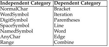
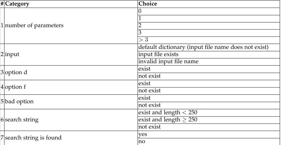
For the programs taken from the SIR, and the Unix utilities, limited documentation was available, so we in-ferred the behavior of each program by examining the test inputs and outputs, as well as the source code. To avoid a possible source of bias, while designing categories and choices, we did not examine the faults. As noted previously, our categories and choices forgrepwere designed to test its regular expression analyzer. To obtain these, we consulted the user documentation.
Precise details on the categories and choices used in our study are provided in Tables A4 to A15 in the Appendices.
4.5 Generation of test cases for object programs
few thousand test cases per program) to ensure sufficient randomness. Thus, rather than sampling test cases from the existing pools, we used a number of techniques to dynami-cally generate test cases on demand. Our approach has some similarities to fuzz testing. We first analyzed the existing test pools to obtain the probability distributions of certain parameters. Then, according to the probability distributions, the concrete values of these parameters could be randomly chosen. The detailed procedure for test case generation for each object program can be found in Appendix A.
For the Unix utilities, Wong et al. [29] developed a random test case generator, which we used in our study.
For grep, we used a generator that was itself based on the categories and choices devised for ART selection. We systematically generated random candidate test cases, which were collectively guaranteed to cover each category and choice. Our test generator does not randomly sample from the entire input domain ofgrep; rather, it samples a small subset of the input space, as our purpose is to test the regular expression analyzer of grep. We further filtered the randomly generated pool to remove duplicate entries. The final pool contained 171,634 elements. Readers can refer to Appendix B for more technical details on the random test case generation process forgrep.
4.6 Experiment environment
All experiments were conducted on a cluster of 64-bit Intel Clovertown systems running CentOS 5. The large number of experimental trials required to collect data with sufficiently narrow confidence intervals consumed a great deal of com-puter time, making the use of the cluster essential to obtain results in a reasonable time. The object programs were written in standard C and did not require any modifications to compile and run on the nodes in the cluster.
4.7 Experiment design and analysis strategy
4.7.1 Number of candidates
The parameter k — the size of the candidate set used by FSCS-ART — is at the tester’s discretion. Previous work [9] has shown — at least for numeric programs — that failure-detection effectiveness improves askincreases up to about 10, and then does not improve much further. Thus, our experiments were all conducted withkset to 10.
4.7.2 F-measure
For an experiment run, a test case was generated (using RT or ART) and executed on both an unmodified version of the object program under test and a version containing the fault of interest. A failure was indicated by a difference between the outputs of the faulty and original versions. For each fault, 2000 runs were performed for the RT, ARTmif, and ARTsum strategies, and the F-measure was calculated as the mean value of F-counts (refer to Equation 4) across all the experiment runs. This large number of runs is desirable due to the statistical properties of the F-count. Typically, the population distribution of the F-count is geometric for RT and near-geometric for most ART variants [7]; therefore, the standard deviation is very high and obtaining acceptably narrow confidence intervals requires large samples.
Being intended as an enhancement to RT, we calculated the ratio of the F-measure for each ART technique compared to the F-measure for RT for each fault. We refer to this as the F-ratio. The F-measures for RT on different faults in the same object program vary by orders of magnitude, and these F-measures are not normally distributed. Therefore, to con-cisely summarize the differences in performance between the methods, we present the relative performance using RT as the baseline – the F-ratio.
4.7.3 P-measure
Raw data to calculate P-measures was recorded in the same experiments. For each fault in each object program, 2,000 runs of 1,000 test cases were conducted, and fail-ures were recorded. P-measfail-ures were calculated accord-ing to Equation 5 when the number of test cases n = 1,2, . . . ,10,20, . . . ,100,200, . . . ,1000.
The P-measure does not, by itself, provide enough infor-mation to assess a testing strategy if the resulting test suites are of different sizes; thus, a further metric is required. In this study, we used the aggregation of P-measures across various test suite sizes, as measured by the total area under the P-measure graph, namely the “P-measure area”, (ab-breviated as “PMA”). Suppose that P-measures have been calculated forNsdifferent test suite sizes{n1, n2, . . . , nNs}, wheren1< n2< . . . < nNs. PMA is calculated as:
PMA = P-measure(n1)
2 ×n1+
Ns
X
i=2
P-measure(ni) +P-measure(ni−1)
2 ×(ni−ni−1)
(6) As we discuss in Section 5.1.2, a higher PMA was a re-liable indicator that a particular parameterized test strategy was more effective, regardless of test suite size.
4.8 Threats to validity
4.8.1 Internal validity
4.8.2 External validity
The most obvious threat to external validity is that we consider only 14 object programs. We cannot say whether the studied methods will exhibit similar results on other software systems without further study. The selection of appropriate categories and choices is a subjective process relying on the knowledge and experience of the testers (which were the authors). Our study considered only one set of categories and choices for each object program. We cannot be sure that other testers, presented with the same software under test, would choose a set of categories and choices that would achieve similar results. The particular faults we used, almost all of which were the result of fault seeding by programmers or randomly applying mutation operators, may not be representative of real faults and fault distribu-tions encountered in industrial practice. A further threat to external validity involves our considering the detection of a single fault at a time. There is no reason why the same intuition that explains why ART detects single faults more quickly than RT should not also hold when multiple faults are present; however, this needs to be assessed empirically.
4.8.3 Construct validity
As discussed in Section 4.3.2, none of the metrics used here give a full picture of the fault-finding effectiveness of a test-ing technique. They all measure failure-detection capability, but do not directly measure the ability of a technique to detect multiple faults in the software under test.
4.8.4 Conclusion validity
Given the large number of experiment runs conducted for each fault, we believe that our tests had sufficient statistical power to draw conclusions about the F-measures and P-measures of each testing strategy at the individual fault level. However, the use of weaker nonparametric tests for statistical significance has limited our ability to show signif-icant differences where they may exist.
5
D
ATA AND ANALYSIS5.1 RQ1: Failure-detection effectiveness
5.1.1 F-measure
For each object program, we present a boxplot and a table summarizing the results. The boxplot for each program (Figure 1) graphically displays the range of F-ratios through their quartiles for each of the two ART methods, for all faulty versions of the program under test. Smaller F-ratios indicate better performance for ART, and an F-ratio smaller than 1 indicates that ART outperformed RT. The boxplot is non-parametric, that is, there is no underlying assumption of statistical distributions. The lower and upper sides of the box denote the lower and upper quartiles respectively. The line inside the box indicates the median F-ratio. The whiskers represent the smallest and largest data within a range±1.58×IQR, whereIQRis the interquartile range. Small circles represent outliers outside this range. Full re-sults are given in Tables A16 to A29 in the Appendices.
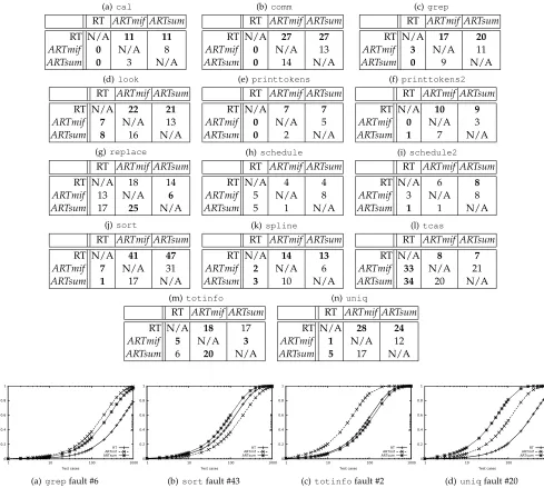
Table 5 presents direct pairwise comparisons of the F-measures of RT, ARTsum, and ARTmif for each object pro-gram. Each cell in the table represents the number of faults
on which the technique listed abovethe cell outperformed the technique listed to the left. For instance, in Table 5(a), the entry in the top right-hand corner of the table shows that ARTmif had asmaller F-measure than RT on all 11 of the faults. Similarly, the entry in the bottom left-hand corner shows that RT outperformedARTsumon 0 of the 11 faults.
Because the number of faults for each object program was small and their F-measures were not normally dis-tributed, conventional parametric hypothesis testing (such as T-tests or ANOVAs) is not suitable for analyzing our re-sults [16]. Thus, to test whether the performance differences were statistically significant, we conducted a Friedman test for each method. The Friedman test [14] examines whether the rankings of the methods across trials (faults, in this case) are as would be expected if they were sampled from the same population. To use an overall α (probability of a non-significant difference being incorrectly classified as significant) of 0.05 across the entire paper, we used the Holm-Bonferroni method [19] to determine which programs exhibited statistically significant differences. Note that in the nonparametric statistical test, it is irrelevant whether we use the F-ratio or the unadjusted F-measure, as the ranking is unaffected. On all programs exceptschedule, the testing methods exhibited failure-detection results that were statis-tically significantly different. To determine which methods performed significantly differently for each fault, post-hoc comparisons using the Wilcoxon signed-rank test [28] with corrections for multiplicity were used. Aboldnumber in the tables indicates that the differences between methods was statistically significant. For instance, the fact that ARTmif outperformed RT on 17 of the 20grepfaults is statistically significant, whereas the fact that ARTsum outperformed ARTmif on 11 of the 20grepfaults is not.
ARTsumsignificantly outperformed RT in terms of the F-measure on 10 of the 14 object programs. For three of the remaining four programs, replace, schedule, and totinfo, there was no statistically significant difference in the performance ofARTsumand RT. On only one program, tcas, did RT significantly outperformARTsum.
ARTmif displayed similar but not identical perfor-mances. ARTmif outperformed RT on 10 of the 14 object programs. There were no statistically significant differences in performance on three programs, replace,schedule, andschedule2. Again, only on tcasdid RT outperform ARTmif. The magnitude of the performance improvement varied between programs. The differences in effectiveness between ARTsum and ARTmif were small. There was a slight preponderance of results indicating thatARTsummay marginally outperform ARTmif, but these did not achieve statistical significance.
5.1.2 P-measure
Figure 2 shows the P-measure for the three techniques for selected faults to illustrate general trends in the results. Note the use of logarithmic scales on the x-axis in Figure 2 to enable the three techniques to be distinguished for small test suite sizes.
ARTmif ARTsum
0.0
0.2
0.4
0.6
0.8
1.0
(a)cal
ARTmif ARTsum
0.0
0.2
0.4
0.6
0.8
1.0
(b)comm
●
● ● ●
ARTmif ARTsum
0.0
0.5
1.0
1.5
(c) grep
● ● ● ● ●
● ●
● ●
ARTmif ARTsum
0.0
0.5
1.0
1.5
2.0
(d)look
ARTmif ARTsum
0.0
0.2
0.4
0.6
0.8
1.0
(e)printtokens
●
ARTmif ARTsum
0.0
0.5
1.0
1.5
(f)printtokens2
ARTmif ARTsum
0
1
2
3
4
(g)replace
ARTmif ARTsum
0
1
2
3
4
5
(h)schedule
ARTmif ARTsum
0.0
0.5
1.0
1.5
(i)schedule2
●
●
ARTmif ARTsum
0.0
0.5
1.0
1.5
2.0
(j)sort
● ●
● ●
ARTmif ARTsum
0.0
0.5
1.0
1.5
2.0
(k)spline
ARTmif ARTsum
0.0
0.5
1.0
1.5
2.0
2.5
(l)tcas
ARTmif ARTsum
0.0
0.5
1.0
1.5
(m)totinfo
● ●
ARTmif ARTsum
0.0
0.5
1.0
1.5
(n)uniq
TABLE 5
Number of Faults for Which the Technique on the Top Row Has a Lower (Better) F-measure Than the Technique on the Left
(a)cal
RT ARTmif ARTsum
RT N/A 11 11
ARTmif 0 N/A 8
ARTsum 0 3 N/A
(b)comm
RT ARTmif ARTsum
RT N/A 27 27
ARTmif 0 N/A 13
ARTsum 0 14 N/A
(c)grep
RT ARTmif ARTsum
RT N/A 17 20
ARTmif 3 N/A 11
ARTsum 0 9 N/A
(d)look
RT ARTmif ARTsum
RT N/A 22 21
ARTmif 7 N/A 13
ARTsum 8 16 N/A
(e)printtokens
RT ARTmif ARTsum
RT N/A 7 7
ARTmif 0 N/A 5
ARTsum 0 2 N/A
(f)printtokens2
RT ARTmif ARTsum
RT N/A 10 9
ARTmif 0 N/A 3
ARTsum 1 7 N/A
(g)replace
RT ARTmif ARTsum
RT N/A 18 14
ARTmif 13 N/A 6
ARTsum 17 25 N/A
(h)schedule
RT ARTmif ARTsum
RT N/A 4 4
ARTmif 5 N/A 8
ARTsum 5 1 N/A
(i)schedule2
RT ARTmif ARTsum
RT N/A 6 8
ARTmif 3 N/A 8
ARTsum 1 1 N/A
(j)sort
RT ARTmif ARTsum
RT N/A 41 47
ARTmif 7 N/A 31
ARTsum 1 17 N/A
(k)spline
RT ARTmif ARTsum
RT N/A 14 13
ARTmif 2 N/A 6
ARTsum 3 10 N/A
(l)tcas
RT ARTmif ARTsum
RT N/A 8 7
ARTmif 33 N/A 21
ARTsum 34 20 N/A
(m)totinfo
RT ARTmif ARTsum
RT N/A 18 17
ARTmif 5 N/A 3
ARTsum 6 20 N/A
(n)uniq
RT ARTmif ARTsum
RT N/A 28 24
ARTmif 1 N/A 12
ARTsum 5 17 N/A
0 0.2 0.4 0.6 0.8 1
1 10 100 1000
P-measure
Test cases RT ARTmif ARTsum
(a)grepfault #6
0 0.2 0.4 0.6 0.8 1
1 10 100 1000
P-measure
Test cases
RT ARTmif ARTsum
(b)sortfault #43
0 0.2 0.4 0.6 0.8 1
1 10 100 1000
P-measure
Test cases RT ARTmif ARTsum
(c)totinfofault #2
0 0.2 0.4 0.6 0.8 1
1 10 100 1000
P-measure
Test cases RT ARTmif ARTsum
(d)uniqfault #20
Fig. 2. P-measure by technique for selected faults.
complete picture. To enable the statistical analysis of the P-measure results, we used PMA (as defined in Section 4.7.3) to aggregate results enabling us to compare the effectiveness of testing methods. For a given fault, if PMA is larger for a methodαthan for another methodβ, the performance ofα is superior to that ofβ. Figure 2 clearly shows that for the selected faults, if one method has a higher P-measure and is therefore more effective than another for a given test suite size, then it will be equal to or superior than the other for other test suite sizes. This pattern holds for all faults.
We calculated the PMA for all faults in all programs and ranked the methods for each fault in each program, and conducted Friedman tests (applying a Holm-Bonferroni correction across all hypothesis tests, for both P-measures and F-measures) to check the statistical significance of the rankings. Our results showed that, in virtually all cases,
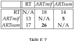
if one method demonstrated a superior (lower) F-measure than another for a specific fault in a program, that method would have a superior (higher) PMA, and that the differ-ences that were statistically significant for the P-measures and F-measures were identical. The rankings of F-measure and P-measure are almost the same, with a slight difference only forreplaceas given in Table 6. The complete PMA’s rankings are given in Table A30 in the Appendices.
5.2 RQ2: Test suite generation time
0 2 4 6 8 10 12 14
0 2000 4000 6000 8000 10000
time (s)
size of test suite RT ARTmif ARTsum (a)printtokens 0 0.5 1 1.5 2 2.5 3 3.5 4
0 2000 4000 6000 8000 10000
time (s)
size of test suite RT ARTmif ARTsum (b)schedule 0 2 4 6 8 10 12 14
0 2000 4000 6000 8000 10000
time (s)
size of test suite RT
ARTmif ARTsum
(c)grep
Fig. 3. Time required to generate test suites
TABLE 6
Number of Faults for Which the the Technique on the Top Row has a Higher (Better) PMA Than the Technique on the Left forreplace
RT ARTmif ARTsum
RT N/A 18 14
ARTmif 13 N/A 5
ARTsum 17 26 N/A
TABLE 7
Comparison of Time Required to Generate 10,000 Random Inputs Using RT,ARTmifandARTsum
Generation time (s) Relative generation time
RT ARTmif ARTsum ARTmif RT
ARTsum RT
ARTsum ARTmif cal 0.032 0.15 0.065 4.7 2.0 2.3
comm 0.034 0.222 0.117 6.5 3.4 1.9
grep 0.011 23.122 0.064 2102.0 5.8 361.3
look 0.023 0.368 0.105 16.0 4.6 3.5
printtokens0.421 13.365 3.046 31.7 7.2 4.4
replace 0.018 2.264 0.146 125.8 8.1 15.5
schedule 0.052 3.637 0.331 69.9 6.4 11.0
spline 0.022 0.622 0.116 28.3 5.3 5.4
sort 0.011 2.717 0.072 247.0 6.5 37.7
tcas 0.018 2.306 0.104 128.1 5.8 22.2
totinfo 0.045 1.464 0.3 32.5 6.7 4.9
uniq 0.025 0.839 0.1 33.6 4.0 8.4
Table 7 shows these constant factors by indicating the time required to generate 10,000 test cases using RT for all the input generators. Note thatscheduleandschedule2 share the same input generator, as do printtokens and printtokens2, so only 12 input generators are listed. We also compare the relative time taken using the three different methods for each input generator. As can be seen, there is wide variation in the relative time costs of input generation depending on the program. The generation time using the ARTsumalgorithm are within a range of 2.0 to 8.1 times that of RT, whereasARTmif takes 4.7 to 2102.0 times longer than RT and takes 1.9 to 361.3 times longer thanARTsum.
6
D
ISCUSSIONOverall,ARTsumandARTmif were clearly each more effec-tive than RT, as measured by both the F-measure and P-measure, on a majority of the object programs considered. ARTsum also had a much lower selection overhead than ARTmif, and its overhead was close to that of RT.
We examined the cases in which ARTsumwas not sig-nificantly more effective in terms of fault-detection than RT. This occurred on the object programsreplace,schedule, and totinfo, where differences betweenARTsumand RT were not statistically significant, and on tcas, where RT was more effective than ART. Our investigation revealed an interesting pattern related to the distribution of failure-revealing inputs in test frames for the different faulty ver-sions ofreplace. We first examined the failure rate within failure-revealing “test frames” – that is, the subsets of the test pool that shared the same categories and choices, and contained at least one failure-causing input. We hypothe-sized that for faults on which ART performed poorly, the failure rate within the failure-revealing test frame would be lower. There did not appear to be any such systematic effect, so we then examined the distribution of the test frames containing failure-causing input in terms of their average “distance”. We found that the “distance” between frames containing failures was higher for faults on which ART outperformed RT, and lower when RT outperformed ART. The faulty versions ofscheduleandtcas, on which ART exhibited comparatively poor performance, have similar distributions of failure-revealing inputs in test frames.
been observed in previous studies of ART. In fact, biases are almost inevitable; it is difficult to achieve an effective spreading of inputs without inducing some bias towards certain inputs. ARTmif preferentially selected inputs that had a large number of choices. For each of the three faults in grep on which ARTmif did not outperform RT, most of the failure-causing inputs had a very small number of choices. Hence, these failure-causing inputs were less likely to be selected by ARTmif than by random chance. This is related to the granularity problems of the distance measure as discussed in Section 3.2, but is not strictly the same. The same phenomena affect the results for individual mutants of the same program. This combined with the relatively small number of mutants per program, is probably responsible for a few unusual looking boxplots in Figure 1.
We have shown thatARTsumsignificantly outperformed RT on 10 of our 14 object programs. Our results showed that ARTsumandARTmifhad comparable performance, and that ARTsum slightly outperformed ARTmif particularly when there were a small number of categories. However, this is consistent with our view that the max-sum criterion handles a coarse distance measure better than the max-min criterion. We have clearly shown that while bothARTsumand ART-mifare linear-time algorithms, in practice,ARTsumcan incur a much smaller selection overhead thanARTmif. Therefore, given that ARTsum and ARTmif have comparable failure-detection effectiveness, the lower overhead suggests that ARTsumshould be considerably more cost-effective overall. Despite the satisfactory effectiveness demonstrated by the “forgetting” strategies employed inARTmifin this study as well as prior studies, the settings of their parameters seem to be arbitrary and are not rigorously justified. This arbitrariness does not occur forARTsum, which in our view is a further reason to prefer it toARTmif.
Selecting categories and choices for ART may impose an additional burden on the tester, compared to RT. It is true that the selection of appropriate categories and choices may not always be straightforward, and may depend substan-tially on the tester’s expertise and experience. If random test cases could be easily generated, RT might be more cost-effective than ART. Nevertheless, in many practical situa-tions, especially when the software under test involves more complicated inputs (such as those with non-numeric types), it is not straightforward to randomly generate test cases. As noted by Arcuri et al. [5, pg. 261], “[w]hen the input domain consists of numeric inputs, it is easy to uniformly choose random test cases from it. But it is not always clear how to do that when more complex types of test cases are used.” To apply RT to a non-numeric input domain, testers may need to perform some analysis of the input domain. One useful method for doing so is by identifying categories and choices, just as has been done in this paper. If such an approach has been taken, the additional effort by testers to apply ART over RT would be small.
Another interesting issue is that whileARTsumcan gen-erate test cases in linear time, its test case generation time is still several times longer than RT. This implies that RT may be more cost-effective than ARTsumunder particular conditions, especially when test execution time is negligible. However, the execution of test cases often takes a substantial amount of time, particularly once the time taken for testing
infrastructure such as setup, teardown, and result reporting is taken into account. In such a situation, the larger number of test cases required by RT would result in longer overall testing time than ARTsum. For example, one of our object programs, grep, on average took 2.98×10⁻⁴ seconds to execute a test case. On average, RT required 1.1 ×10⁻⁶ seconds, andARTsumtook6.4×10−6seconds, to generate one test case. For grep, therefore, the cost of performing testing is dominated by the cost of test case execution. The ratio of total testing time taken by ART over RT was thus very similar to the F-ratio. For example, on the first mutant of grep, ARTsum took 1.33×10⁻² seconds, whereas RT took 3.10×10⁻² seconds. There is no “golden method” that always has higher-cost effectiveness than other testing methods for all programs. Indeed, RT can be better than ARTsumunder some conditions, such as in cases involving high failure rates and short program execution time. In this paper, we intend to provide a testing method for programs that have non-numeric inputs requiring systematic analysis, and that have long execution times. For such situations, it is very likely thatARTsumis more cost-effective than RT.
7
R
ELATEDW
ORKThe extension of ART to non-numeric input domains has been of interest for some time. Ciupa et al. [11] demon-strated the application of ART to unit testing of object-oriented software. There are significant differences between their approach and ours. Ciupa et al.’s distance measure, which was specifically designed for unit testing of object-oriented software, is based on the structure of method inputs, and permits no tester discretion. Our distance mea-sure, in contrast, allows testers to use their knowledge of the specification and/or the program structure to specify appropriate categories and choices. It is not restricted to object-oriented languages, and is applicable beyond unit testing. Ciupa et al.’s implementation uses FSCS-ART as the test case selection technique. This technique’s quadratic selection overhead implies that overall, ART might not actually be cost effective compared to random testing. Our technique, in contrast, takes advantage of the properties of our distance measure to achieve linear-time selection overhead, addressing these cost-effectiveness issues.
There have been a number of attempts to reduce the selection overhead of ART, even before Arcuri and Briand [3] drew attention to the implications of this for the prac-tical use of ART. For instance, Shahbazi et al. [25] devised RBCVT-Fast, a linear-time ART algorithm ford-dimensional real input domains. Our work is complementary to theirs in that it can be applied to non-numeric input domains.
may not be sufficient compensation for a much longer test case generation time. In addition, no testing method is guaranteed to detect all types of faults. The “systematic” methods may be very effective in detecting certain types of faults, but they may also be very ineffective in the detection of other faults. Random strategies (such as RT and ART) can be considered to be complementary to them: due to the randomness, random strategies can detect some faults difficult to detect using systematic methods [4], [5], [17]. As mentioned in Section 6, there is no “golden method”. Any testing method has its own advantages and disadvantages, dependent on various factors, in particular, the program execution time which can vary enormously. The ARTsum method proposed in this paper can be considered as a possible cost-effective enhancement to RT and a good com-plementary testing method to other systematic ones, when the software under test involves non-numeric and struc-tured inputs. ART is complementary to other systematic testing methods not only because ART and other methods can work independently to detect different types of faults, but also because they can be integrated to provide hybrid techniques. For example, ART has been used to improve the test cases’ diversity in model-based testing [18]. It would be worthwhile to systematically compare ART with other state-of-the-art testing techniques, but such an experimental comparison is beyond the scope of this paper (in which we focus on how to improve RT) and is one important direction for the future work.
There are some obvious parallels between some aspects of combinatorial testing [23] and our ART algorithm. But there are some fundamental differences. Combinatorial test-ing has coverage as its underlytest-ing notion, and aims to de-tect faults that are related to interactions between different parameters. The underlying concepts of ART, in contrast, are randomness and diversity across the input domain. ART does not involve any form of coverage of specific combinations of parameters, and combinatorial testing does not involve randomness and diversity across the input domain. From an operational perspective, ART normally generates test cases in an incremental way, while combi-natorial testing fundamentally requires the generation of an entire test suite that satisfies certain coverage criteria, such as t-way combinations. In other words, the combinatorial testing has a lower bound on how many test cases should be generated, while ART can generate any number of test cases until a termination condition is satisfied. The incremental nature of ART is actually an advantage over combinatorial testing, especially when there are many factors that must be considered in testing. For example, a complex system (such asgrep) can involvenfunctionalities, each of which may be associated withmoptions and thenpsub-options. Such a hierarchy in inputs can result in a very large input space. In addition, there may be an “explosion” in the input space: The lower bound in test suite size of combinatorial testing will increase exponentially as the values ofm,nand p increase. Our work addresses this “explosion” problem by a simple method: The distance measure we proposed treats the input space in two flat layers – the input space is partitioned into different categories and their associated choices. The numbers of categories and choices do not necessarily grow with the increase ofm,n, andp, and there
are common categories and choices across different func-tionalities, options, and sub-options. Even if the numbers of categories and choices become larger with the growth of the input domain, due to its incremental nature, ART does not suffer from the input space “explosion” problem: ART im-poses no rigid requirements on the test suite size no matter how large the input space is. Such fundamental differences make it extremely difficult, if not impossible, to compare ART and combinatorial testing using the F-measure. The measurement of P-measure had a similar problem: Both RT and ART have high flexibility in test case generation, making it possible to obtain P-measure values with various test suite sizes; by contrast, combinatorial testing imposes fixed test suite sizes.
8
C
ONCLUSIONART was proposed to enhance the failure-detection effec-tiveness of RT. In this work we have presented a linear-order ART algorithm, ARTsum, that makes use of a novel distance measure, and takes advantage of the properties of this distance measure to achieve a linear-order test case gen-eration. Our work is complementary to the recent RBCVT-Fast algorithm [25], which is an innovative linear-order ART algorithm for numeric inputs.
We conducted an empirical study using a total of 14 programs, comparing our ARTsumalgorithm with RT and a baseline ART technique using the max-min criterion and the technique of “forgetting” to reduce selection overhead, namely ARTmif. Each of the ART algorithms significantly outperformed RT with respect to the F-measure for 10 of the 14 object programs, was significantly outperformed by RT for only one program, and had performance comparable to that of RT for the remaining three programs. An almost identical pattern was observed for the P-measure. Further-more, the selection overhead ofARTsumwas quite close to that of RT, and far lower than that ofARTmif.
R
EFERENCES[1] V. D. Agrawal. When to use random testing. IEEE Transactions on Computers, 27(11):1054–1055, 1978.
[2] P. E. Ammann and J. C. Knight. Data diversity: An approach to software fault tolerance.IEEE Transactions on Computers, 37(4):418– 425, 1988.
[3] A. Arcuri and L. Briand. Adaptive random testing: An illusion of effectiveness? InProceedings of the 20th International Symposium on Software Testing and Analysis, ISSTA ’11, pages 265–275, 2011. [4] A. Arcuri, M. Z. Iqbal, and L. Briand. Black-box system testing of
real-time embedded systems using random and search-based test-ing. InProceedings of the 22nd IFIP WG 6.1 International Conference on Testing Software and Systems, ICTSS ’10, pages 95–110, 2010. [5] A. Arcuri, M. Z. Iqbal, and L. Briand. Random testing: Theoretical
results and practical implications. IEEE Transactions on Software Engineering, 38(2):258–277, 2012.
[6] K.-P. Chan, T. Y. Chen, and D. Towey. Forgetting test cases. In Proceedings of the 30th Annual International Computer Software and Applications Conference, COMPSAC ’06, pages 485–494, 2006. [7] T. Y. Chen, F.-C. Kuo, and R. Merkel. On the statistical properties
of testing effectiveness measures. Journal of Systems and Software, 79(5):591–601, 2006.
[8] T. Y. Chen, F.-C. Kuo, R. Merkel, and S. P. Ng. Mirror adaptive random testing. Information & Software Technology, 46(15):1001– 1010, 2004.
[9] T. Y. Chen, H. Leung, and I. K. Mak. Adaptive random testing. InProceedings of the 9th Asian Computing Science Conference, pages 320–329, 2004.
[10] T. Y. Chen and R. Merkel. Quasi-random testing.IEEE Transactions on Reliability, 56(3):562–568, 2007.
[11] I. Ciupa, A. Leitner, M. Oriol, and B. Meyer. ARTOO: Adaptive random testing for object-oriented software. In Proceedings of the 30th International Conference on Software Engineering, ICSE ’08, pages 71–80, 2008.
[12] M. E. Delamaro and J. C. Maldonado. Proteum – a tool for the assessment of test adequacy for C programs. InProceedings of the Conference on Performability in Computing Systems, PCS ’96, pages 79–95, 1996.
[13] H. Do, S. G. Elbaum, and G. Rothermel. Supporting controlled experimentation with testing techniques: An infrastructure and its potential impact. Empirical Software Engineering: An International Journal, 10(4):405–435, 2005.
[14] M. Friedman. The use of ranks to avoid the assumption of nor-mality implicit in the analysis of variance. Journal of the American Statistical Association, 32(200):675–701, 1937.
[15] J. D. Golic. New methods for digital generation and postprocess-ing of random data. IEEE Transactions on Computers, 55(10):1217– 1229, 2006.
[16] F. J. Gravetter and L. B. Wallnau.Statistics for the Behavioral Sciences. West Publishing Company, 1996.
[17] A. Groce, G. J. Holzmann, and R. Joshi. Randomized differential testing as a prelude to formal verification. InProceedings of the 29th International Conference on Software Engineering, ICSE ’07, pages 621–631, 2007.
[18] H. Hemmati, A. Arcuri, and L. Briand. Achieving scalable model-based testing through test case diversity. ACM Transactions on Software Engineering and Methodology, 22(1):6:1–6:42, 2012. [19] S. Holm. A simple sequentially rejective multiple test procedure.
Scandinavian Journal of Statistics, 6:65–70, 1979.
[20] F.-C. Kuo. On Adaptive Random Testing. PhD thesis, Faculty of Information and Communication Technologies, Swinburne Uni-versity of Technology, 2006.
[21] Y. Liu and H. Zhu. An experimental evaluation of the reliability of adaptive random testing methods. In Proceedings of the 2nd International Conference on Secure System Integration and Reliability Improvement, SSIRI ’08, pages 24–31, 2008.
[22] R. Merkel. Analysis and Enhancements of Adaptive Random Testing. PhD thesis, School of Information Technology, Swinburne Univer-sity of Technology, 2005.
[23] C. Nie and H. Leung. A survey of combinatorial testing. ACM Computing Surveys, 43(2):11:1–11:29, 2011.
[24] T. J. Ostrand and M. J. Balcer. The category-partition method for specifying and generating functional tests. Communications of the ACM, 31(6):676–686, 1988.
[25] A. Shahbazi, A. F. Tappenden, and J. Miller. Centroidal voronoi tessellations — a new approach to random testing. IEEE Transac-tions on Software Engineering, 39(2):163–183, 2013.
[26] The GNU Project. Grep home page. http://www.gnu.org/ software/grep, 2006.
[27] L. J. White and E. I. Cohen. A domain strategy for computer pro-gram testing. IEEE Transactions on Software Engineering, 6(3):247– 257, 1980.
[28] F. Wilcoxon. Individual comparisons by ranking methods. Biomet-rics Bulletin, 1(6):80–83, 1945.
[29] W. E. Wong, J. R. Horgan, S. London, and A. P. Mathur. Effect of test set minimization on fault detection effectiveness. Software: Practice and Experience, 28(4):347–369, 1998.
[30] B. Zhou, H. Okamura, and T. Dohi. Enhancing performance of random testing through markov chain monte carlo methods.IEEE Transactions on Computers, 62(1):186–192, 2013.
Arlinta Barus is a Lecturer at Del Institute of Technology, Indonesia. She received her Bache-lor degree in Informatics Engineering from Ban-dung Institute of Technology, Indonesia, Master degree in Information Communication and Tech-nology from the University of Wollongong, and PhD degree from Swinburne University of Tech-nology. Her current research interest is mainly in software testing.
Tsong Yueh Chenis a Professor at Swinburne University of Technology. He received his PhD in Computer Science from The University of Mel-bourne, the MSc and DIC from Imperial College of Science and Technology, and BSc and MPhil from The University of Hong Kong. He taught at The University of Hong Kong and The University of Melbourne. His main research interest is on software testing.
Fei-Ching Kuo is a Senior Lecturer at Swin-burne University of Technology, Australia. She received her Bachelor of Science Honors in Computer Science and PhD in Software Engi-neering, both from Swinburne University of Tech-nology, Australia. She was a lecturer at Univer-sity of Wollongong, Australia. Her current re-search interests include software analysis, test-ing and debuggtest-ing.
Huai Liuis a Research Fellow at the Australia-India Research Centre for Automation Software Engineering, RMIT University, Australia. He re-ceived the BEng and MEng both from Nankai University, China, and the PhD degree in soft-ware engineering from the Swinburne University of Technology, Australia. His current research interests include software testing, cloud comput-ing, and end-user software engineering.
Robert Merkelis a Lecturer at Monash Univer-sity, Melbourne, Australia. He received his PhD degree from the Swinburne University of Tech-nology. His research interests include software testing and software reliability.