Intercomparison between Switch 2.0 and
GE MAPS models for simulation of
high-renewable power systems in Hawaii
Matthias Fripp
1,*1 University of Hawaii, Department of Electrical Engineering, Honolulu, Hawaii 96822, USA
ABSTRACT
Background: New open-source electric-grid planning models have the potential to improve power system planning and bring a wider range of stakeholders into the planning process for next-generation, high-renewable power systems. However, it has not yet been established whether open-source models perform similarly to the more established commercial models for power system analysis. This reduces their credibility and attractiveness to stakeholders, post-poning the benefits they could offer. In this paper, we report the first model intercomparison between an open-source power system model and an established commercial production cost model.
Results: We compare the open-source Switch 2.0 to GE Energy Consulting’s Multi Area Pro-duction Simulation (MAPS) for proPro-duction-cost modeling, considering hourly operation under 17 scenarios of renewable energy adoption in Hawaii. We find that after configuring Switch with similar inputs to MAPS, the two models agree closely on hourly and annual production from all power sources. Comparing production gave a coefficient of determination of 0.996 across all energy sources and scenarios, indicating that the two models agree on 99.6% of the variation. For individual energy sources, the coefficient of determination was 69–100.
Conclusions: Although some disagreement remains between the two models, this work indi-cates that Switch is a viable choice for renewable integration modeling, at least for the small power systems considered here.
Keywords: model intercomparison, renewable energy, production cost modeling, security-constrained unit commitment, open-source software
Background
Recent research indicates that human society must begin reducing greenhouse gas emissions sharply by 2020 and reach zero net emissions by 2040–55 in order to prevent dangerous climate change [1]. The elec-tricity sector will likely play a key role in this transition, absorbing renewable power and distributing it to traditional loads and electrified heating and transport sectors [2]. Achieving this transition at least cost will require widespread analysis and optimization of high-renewable power system designs, integrated with the surrounding economy.
In recent years, several new, open-source or academic power system models have been introduced to aid in this effort [3–18]. These models are publicly documented and available at no cost, enabling a wide range of stakeholders to propose and assess transition plans, often integrated with broader economic modeling. However, most renewable energy integration studies to date have used closed-source, proprietary models, e.g., [19–27]. These proprietary models are generally written and run by well-known firms in the power industry, and over the years they have built up a store of confidence among electricity planners. This confi-dence comes from a history of benchmarking against existing power systems, repeated use for a wide variety of studies, and backing by respected firms. However, established, commercial models are only available at high cost; do not use public, peer-reviewed formulations; and are not easily extendable for integration into broader economic modeling.
This leaves a gap in our ability to plan for high-renewable power systems. Open-source and academic models have sound, peer-reviewed formulations; are accessible and transparent enough to support consensus-building among a variety of stakeholders; and can be integrated with larger economic models to conduct advanced modeling of high-renewable economies [4, 28–30]. However, power system planners are not yet confident that the open and academic models accurately represent power system operations. On the other hand, power system operators are confident in using proprietary power system models, but those models are not transparent or accessible enough to support consensus-building and integrated energy-economic model-ing.
This work seeks to bridge this gap, comparing results from one of the most capable open-source planning models—Switch 2.0—against one of the best-established proprietary power system models—GE Energy Consulting’s Multi Area Production Simulation (MAPS)—when modeling operation of a high-renewable power system in Hawaii. The primary goal is to test whether the open-source model produces similar results to the established, benchmarked model, in order to help users judge whether it is accurate enough for their work. As a secondary goal, this research also tests the replicability of work previously done with the propri-etary model, a key element of the scientific process [29, 31, 32].
In other fields, especially climate modeling, intercomparisons between models are common, either to benchmark the accuracy of different models [33–35] or to identify areas of consensus and disagreement among the models [36–39]. This study takes the former approach, focusing on the question of whether a new, open-source model is able to provide similar results to an established and validated commercial model when modeling a real-world power system. There has also been a serious effort in psychology and other social sciences fields in recent years to test the replicability of previously published findings, in order to ensure the soundness of the field’s work [31, 32]. This paper also makes a small contribution along these lines, testing whether results reported from a proprietary, industry-standard model can be replicated using an open, peer-reviewed model [29].
Switch is an open-source and peer-reviewed model for power systems with large shares of renewable power, storage and demand response. It can run in either capacity-expansion mode (choosing an optimal power system design directly) or production-cost mode (evaluating the cost of running a pre-specified power system design). In this work, we focus on production-cost modeling, which is vitally important to power system operators and is one of the main strengths of existing, proprietary power system models. Switch was released as open-source software in 2008 [13, 40], and has subsequently been used for a number of long-term studies of renewable energy adoption [41–47]. Here we test Switch version 2.0, which was released in 2018 [3, 48].
MAPS is a commercial-grade power system production-cost model that has been widely used for renew-able integration studies in Hawaii and elsewhere [19, 24, 25, 49–56]. It has also been calibrated against system operations in Oahu and Maui [57, 58], giving an extra element of “ground truth” to its findings.
We are not aware of any previous model intercomparison between open-source and commercial grid planning software, especially focusing on renewable energy integration. This gap may be partly because open-source grid planning models have only become widely available in recent years, and partly because few researchers have access to the inputs and assumptions that are needed to replicate professional integration studies. It also requires a great deal of effort to setup a second model to perform a benchmarking study, and resources are rarely available to do this even if it can significantly improve confidence and understanding of both models and their findings. This study takes advantage of the unusual fact that comprehensive data are available on the inputs, assumptions and findings from the MAPS model, as run for the Hawaii Renewable
Portfolio Standards Study (RPS Study) [59], and that Switch 2.0 has also been configured to model the same
power system in order to support planning for the state’s 100% renewable portfolio standard [46].
By necessity this study is deep rather than broad, comparing fine details of the behavior of these two models in one particular region, as reported in the RPS Study. We are not able to compare Switch to other proprietary models or locations because complete reports of inputs and assumptions are not available for other models or locations. We are also unable to compare Switch to MAPS for factors that were not reported in the RPS Study, because we do not have access to all of the MAPS outputs.
Methods
Switch normally uses mixed-integer optimization methods for unit commitment and dispatch. MAPS uses linear optimization methods for unit commitment, with heuristic rules to enforce integer decision vari-ables. For the RPS Study [59], MAPS was specially configured to match the Hawaiian Electric Companies’ heuristic unit commitment rules. The RPS Study report included a substantial body of information about how MAPS was configured, and GE was generous in providing additional data and answers to inquiries. However, the goal of the RPS Study was to evaluate different pathways of renewable integration in Hawaii, rather than to document modeling methods or data, which are constantly evolving. Consequently, we inferred some op-erational details from the figures and results presented in the RPS Study, and in some cases made assumptions that may have differed from ones that MAPS used. The model configuration and inputs used for this study are described below. Switch 2.0 is available from [48]. The data and code used for this model intercomparison are available from [60].
Switch model setup
The Switch model is primarily used as a power system capacity expansion model (co-optimizing selec-tion of new assets and operaselec-tional decisions), but it uses a flexible, modular software framework that allows it to be customized and run as a production cost model (optimizing operational decisions only). For this paper, we run Switch exclusively in production-cost mode, to match the work done with MAPS.
For this intercomparison, we used the following standard Switch modules (documented in more detail in [3]):
• time sampling (we ran Switch with a single month-long timeseries for each month of 2020, with hourly timesteps—12 separate models for each scenario—then aggregated the results); • financial calculations (Switch minimizes costs on an NPV basis, we used a 0% discount rate to
calculate simple costs without discounting);
• generator construction (we specified that the applicable capacity for each of the 17 RPS Study scenarios would be built before the study period and prevented construction of any new capacity during the study);
• generator commitment (this module normally optimizes unit commitment, but we used a cus-tom module described below to force it to follow the heuristic rules used in the RPS Study); • generator dispatch (optimizes generator operation based on fuel prices and variable operation
and maintenance costs);
• operating reserve balancing areas (we setup a pooled reserve balancing area for Oahu and Maui; more details below);
• fuel cost calculations (calculates fuel used by each plant, considering startup requirements, op-erating level and full- and part-load efficiency); and
• transmission construction and operation (we pre-specified the available transmission capacity and allowed operation to be optimized, using a flowgate formulation; more details below). We also used the following custom modules for this study:
• Kalaeloa (shared with other Switch-Hawaii modules; enforces plant-specific unit commitment and production rules for the Kalaeloa combined cycle power plant; more details are below) and • reserves (implements heuristic unit commitment and reserve rules similar to the Hawaiian
Elec-tric rules, as used in MAPS).
For this study, we created 12 monthly models for each of the 17 scenarios, resulting in 204 production cost models to solve. These were solved in about 10 minutes via parallel processing on the University of Hawaii high performance computing system. Total compute time for the 17 scenarios on a single four-core desktop computer would be about four hours. The run-time for MAPS was reported to be under 30 minutes [61].
Thermal generator properties
Operating costs
take-or-pay contract following a fixed schedule, as reported separately by GE [62], and we modeled the independent AES and Kalaeloa plants using representative heat-rate (efficiency) curves as described in [25]. For AES, we used a variable operation and maintenance (O&M) rate of $2 per MWh, as reported in [63]. For Kalaeloa, we set the variable O&M to $8.59/MWh, which resulted in the same full-load operating cost as reported in Figure 30 of the RPS Study [59].
Fixed operating schedules
We configured Switch to follow the same commitment and dispatch schedules as GE described for their model runs [26, 59, 62, 64, 65]. As a general rule, plants identified in the RPS Study as baseload or firm renewable (“firm RE”) were committed (turned on) at all times that they were not out for maintenance. Cy-cling and peaking plants were committed as needed, based on the day-ahead renewable energy forecast. Commitment for peaking plants was further adjusted based on real-time conditions. Firm RE plants also had fixed dispatch (production) schedules [62]. A few plants followed commitment and dispatch schedules that did not fit this general pattern; they are discussed in the supplementary document.
Operating modes for combined-cycle plants
Kalaeloa power plant. The Kalaeloa combined cycle power plant consists of two combustion turbines, one steam turbine powered by waste heat from the combustion turbines. GE modeled these as three units: Kalaeloa 1 and 2 each consisted of one combustion turbine and half of the steam turbine, and Kalaeloa 3 represented additional peaking capacity available if operating in dual-train combined cycle mode [25, 57, 61, 62]. GE also reported that Kalaeloa 3 could operate in quick-start mode if Kalaeloa 1 and 2 were producing at their rated power level. We configured Switch to match this logic, i.e., only allowing Kalaeloa 3 to produce power if Kalaeloa 1 and 2 were at maximum output.
Maalaea combined cycle plants. We modeled each of the Maalaea combined-cycle power plants as two single-train combined cycle generators (a total of four units). Each of these plants consists of two com-bustion turbines and one steam turbine. Based on GE’s reporting, we believed that MAPS modeled these plants as four single-train units. However, GE reported properties for each of these plants on an aggregate basis in the RPS Study report [26]. So we split these properties in such a way that each pair of units would perform the same as the original aggregated plant, if both units were dispatched in tandem.
Minimum Load and Part-Load Heat Rates for Peaking Plants
We modeled peaking plants with no minimum load (meaning they can operate anywhere between 0 and 100% of their rated load), and with a single incremental heat rate for all operating levels, following infor-mation reported separately by GE [62].
Generator Maintenance and Forced Outages
The RPS Study [59] showed Hawaiian Electric’s maintenance schedules, but MAPS used different schedules to avoid interfering with normal operation and reserve margins each week [61]. We inferred the dates of full maintenance outages for most thermal power plants in Oahu by inspection of hourly production data for Oahu plants in Scenarios 2 and 16, which GE provided separately [66]. We assumed that baseload plants were on maintenance or forced outage on all days when they produced zero power. We assumed cy-cling plants were out of service when they produced no power while lower-priority peaking plants produced some power.
We were not able to identify forced outages for peaking plants or Maui plants by this technique. For these plants, we applied the utility’s maintenance schedules shown in the RPS Study [59] and then added random 3-day outages until each plant’s forced outage rate was 2.5% higher than the level shown in Table 7 of the RPS Study [59]. The 2.5% adder was used because we found that outage rates for the Oahu baseload and cycling plants in MAPS were an average of 2.5% higher than the sum of the maintenance schedules and forced outage rates shown in the RPS Study [59].
Fuel Costs
We used fuel costs reported for Oahu and Maui in the RPS Study [59].
Transmission Network
MAPS models transmission using an AC power flow, with DC variations with each commitment and dispatch decision [53, 61]. Switch is normally run with a flowgate-based transmission model, or it can be run with experimental security-constrained AC power flow. Since no network information is available publicly for Oahu and Maui, we ran Switch in flowgate mode, with no congestion or losses within each island, and finite transmission capacity between islands (in grid-tie scenarios). We assumed that all power flows over the grid-tie line incurred losses of 3.8%, based on an analysis of total production values reported for grid-tie and non-grid-tie scenarios in the RPS Study.
Hourly Loads and Renewable Power Production
We used hourly timeseries of renewable production potential, day-ahead forecasts and electricity loads for Oahu and Maui which were provided by GE [67]. Gen-tie wind potential was increased by 5% before applying 5% transmission losses, to achieve consistency with values in the RPS Study.
Spinning Reserve Targets and Allocation
Power systems must keep extra generating capacity committed (turned on) at all times in order to com-pensate for unforeseeable variations in operating conditions. These reserves can be divided into two main “product” categories: contingency reserves, which can compensate for rare events such as loss of a large generator or load; and regulating or operating reserves, which compensate for routine events such as mis-forecast of loads or renewable power. Reserves can also be divided into “up” and “down” directions (availa-ble to increase or decrease production). In Hawaiian power systems, all reserves are usually provided by “spinning” power plants (online and synced to the grid).
Up Reserves
We configured Switch to use the same pre-calculated contingency and regulating reserve targets as MAPS [67]. In the grid-tie scenarios, we divided the regulating reserve target between the two power systems proportional to their hourly load levels; we were not able to identify how MAPS divided this target. We assumed the inter-island grid-tie cable could provide firm power transfers but could not directly provide spinning reserves.
It is not clear from the RPS Study report which power plants were designated to provide up reserves. Based on analysis of several sources [58, 59, 65, 68], we allowed all baseload and cycling units to provide up reserves. Details of our inferences are given in the Supplementary Information. Switch, like MAPS [68], was configured to optimize production levels for individual plants to minimize production cost while respect-ing the overall reserve target.
In the grid-tie scenarios, we configured Switch to divide the regulating reserve target between the Oahu and Maui power systems proportional to their hourly load levels. It is likely that GE used a different method to divide this target, but we were unable to find any documentation of this.
Down reserves
“Down” reserves are provided by power plants that are producing power above their minimum stable or permitted level and are able to reduce production on short notice. We set a contingency down reserve target of 10% of hourly load for Oahu, no regulating down reserve target for Oahu, and no down reserve target of either type for Maui, based on analysis of the RPS Study report [59].
Based on analysis of several sources [25, 26, 59, 68], we divided the down reserve target between re-newable and thermal generators based on their available capacity, and then among individual generators proportional to their committed capacity, as discussed in the Supplementary Information.
Generator Unit Commitment
plants will be committed. For the RPS Study, MAPS was configured to perform a linearized optimization of unit commitment, subject to this ordering, with additional heuristics to ensure integer constraints are satisfied (i.e., units must be fully committed or not at all)[61, 64]. MAPS used two rounds of unit commitment, one based on the day-ahead forecast, and one at real-time, using real-time conditions. All available plants were scheduled in the day-ahead unit commitment, but then peaking plants could be turned on or off as needed in real time [65]. For this study, we configured Switch with a custom commitment algorithm that followed this general approach. In the Supplementary Information we report the assumptions we made about the order of plants in the commitment queues, and the rules that were followed by this commitment algorithm.
Generator Dispatch
For this study, Switch used its standard dispatch methods to choose how much power and reserves to produce from each committed power plant, in order to minimize cost while satisfying the balancing area’s requirements for power and reserves, and respecting constraints on the operation of individual plants (e.g., down-reserve quotas).
Results and Discussion
The commercial GE MAPS production cost model is widely used for renewable energy integration stud-ies, including the recent Hawaii Renewable Portfolio Standards Study (RPS Study) [59]. The goal of this model intercomparison was to test whether similar results could be obtained from the open-source Switch model when studying the same high-renewable power systems. Switch is primarily designed as a capacity expansion model, which means that it selects which assets to build in order to minimize costs while meeting policy objectives. Embedded within this are unit-commitment and dispatch algorithms that decide which plants to turn on each hour and how much power to provide from those plants. MAPS is a production-cost model, which means that it focuses on unit-commitment and dispatch, using pre-specified portfolios of power system assets. Consequently, this model intercomparison focuses only on production-cost analysis. However, this encompasses some of the most important interactions between renewable power, thermal power plants and electricity demand, and these elements underpin Switch’s findings when run in capacity expansion mode. We compared the results from running Switch 2.0 to MAPS for 17 scenarios of interconnection and renewable resource adoption on the islands of Oahu and Maui previously studied with MAPS in the Hawaii
Renewable Portfolio Standards Study (RPS Study) [59]. These had various amounts of wind and solar
gen-erating capacity and various combinations of inter-island transmission cables. Renewable resources ranged from 18 to 55 percent of total energy demand. New transmission options included a “grid-tie cable” to enable bidirectional sharing of power between the Oahu and Maui power systems and/or a “gen-tie” cable to carry power from wind farms on Lanai to the Oahu power system, without connecting to Lanai’s local power system. Scenario 1 in the RPS Study considered the current power systems without significant changes. We configured Switch to match Scenarios 2–18, which represented future power systems. These are summarized in table S1 in the Supplementary Information.
Although the comparisons reported below use quantitative metrics where possible, the comparison is fundamentally qualitative, intended to help researchers identify the areas where the models may differ and attention must be given to produce satisfactory results. We used this approach because statistical significance is not applicable in this context since there is no random variation in the results. It is clear that the models agree closely, but researchers must make their own qualitative judgments of whether they are similar enough to meet their needs.
Annual power production from each class of generator
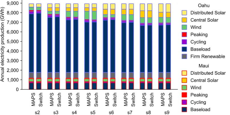
Figures 1 and 2 below show the annual power production from each major type of generator, in each of the 17 scenarios. Different energy sources are stacked in each column, and MAPS and Switch results are compaired in pairs for each scenario. The agreement is generally within 0.5% of total power production for all categories except for baseload production in scenarios the grid-tie-only scenarios, which differ by 1–2%. There are several patterns in the differences between MAPS and Switch (see Fig. 2):
• In the scenarios with a grid-tie cable between the two islands but no gen-tie wind (scenarios 11, 14, 17), Switch uses 120-160 GWh more baseload generation on Oahu than MAPS (1.4–1.9% of total production). It also uses slightly more Maui peaking generation. These are matched by roughly equal decreases in baseload generation on Maui and cycling and peaking generation on Oahu.
• The pattern in the scenarios with gen-tie wind and a grid-tie cable (scenarios 12, 15, 18) is similar to the grid-tie-only scenarios (more Oahu baseload and Maui peaking, less of other thermal plants), but less pronounced. In these scenarios, Switch also curtails more Oahu wind than MAPS and ac-cepts more Maui wind and solar, with a net decrease in renewable production of 0–35 GWh, 0.0– 0.4% of total production.
The coefficient of determination (R2 value) between results from MAPS and Switch across all energy sources and scenarios is 0.9999 for Oahu and 0.9963 for Maui. The R2 value is calculated by computing the square of the correlation coefficient between two vectors. In this case, the first vector was created from all the Oahu or Maui values in the MAPS (left) columns of Figures 1 and 2, and the second vector was created from the corresponding values for Switch (right columns). These R2 values indicate that Switch and MAPS agree on more than 99.5% of the variation between energy sources and scenarios on each island.
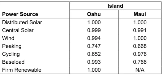
Table 1 shows R2 values across all scenarios for each individual energy source. These values were cal-culated by comparing vectors which each showed the amount of production from one energy source on one island in all 17 scenarios. These indicate how well the Switch and MAPS agree on how production from each individual type of generator varied across the 17 scenarios. The R2 value is above 99% for all the renewable power sources and is 69–100% for the thermal power plants. The lower values for the thermal plants appear to reflect differences in prioritization of the various thermal plants relative to each other, as shown in Figures 1 and 2.
Table 1. R2 value (squared correlation coefficient) between total energy production in MAPS and Switch, across scenarios 2–17, for each power source and island
Power Source
Island
Oahu Maui
Distributed Solar 1.000 1.000
Central Solar 0.999 0.991
Wind 0.994 1.000
Peaking 0.747 0.668
Cycling 0.652 0.976
Baseload 0.993 0.766
Firm Renewable 1.000 N/A
Figure 1. Annual production from each source in scenarios 2–9, as calculated by MAPS and Switch. Up-per, blue-bordered rectangles show Oahu generators; lower, red-bordered rectangles show Maui generators
Figure 2. Annual production from each source in scenarios 10–18, as calculated by MAPS and Switch. Up-per, blue-bordered rectangles show Oahu generators; lower, red-bordered rectangles show Maui generators
Annual Curtailment in Each Scenario
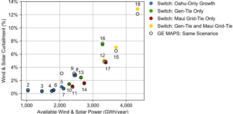
Figure 3 compares the rate of curtailment of renewable power between Switch and MAPS modeling. Curtailment occurs at times when available wind and solar power exceeds system load net of generator min-imum loads and down-reserve requirements. There is one colored marker for each scenario as modeled by Switch, and one black ring for the equivalent scenario in MAPS. The x values for each marker show the amount of wind and solar power that is potentially available in that scenario, found by summing the hourly potential reported by GE in [67]. The y values show the percentage of renewable power that was left unused due to curtailment in each scenario. These calculations include wind, distributed solar and utility-scale solar.
the R2 value between the two models is 0.973, indicating that Switch and MAPS agree on about 97% of the variation in curtailment between scenarios.
The biggest difference is in scenario 5, where Switch has 1.0% curtailment vs. 3.1% for MAPS, driven by curtailment on Oahu, which is 1.0% for Switch and 3.4% for MAPS. We can only investigate this differ-ence indirectly, since we do not have access to the hourly outputs from MAPS for this scenario. The installed resources on Oahu in Scenario 5 are identical to Scenario 10, except that Scenarios 5 has 300 MW of wind on Oahu and Scenario 10 has 100 MW on Oahu and 200 MW on Lanai, connected directly to the Oahu system with a gen-tie cable. Lanai has more wind than Oahu, so the amount of wind power available to the Oahu power system in Scenario 5 is generally slightly lower than in Scenario 10: Oahu wind in Scenario 10 equals or exceeds Scenario 5 during 59% of the year, and average wind during each hour of the day is higher in Scenario 10 than in Scenario 5 for all 24 hours of the day, when averaged over all days of the year. Since Scenario 5 usually has less renewable power available than Scenario 10, we would expect Scenario 5 to have less curtailment than Scenario 10. This is what we found with Switch, but doesn’t match the result from MAPS. However, we are not able to explain the difference further with the data available.
In Scenarios 12, 15 and 18, Switch’s curtailment was 0.2–0.7 percentage points higher than MAPS. These are scenarios with both an inter-island grid-tie cable and Lanai wind connected directly to Oahu via a gen-tie cable. These scenarios have the largest amount of wind power of all the scenarios considered (see Table S1). The total amount of wind power available between midnight and 5 am is 457 GWh in Scenarios 12 and 15 and 521 GWh in Scenario 18, compared to 277–372 GWh in scenarios 10, 11, 13, 14, 16 and 17. This high renewable availability corresponds with higher curtailment during these hours, totaling 87 GWh in Scenario 12, 90 GWh in Scenario 15 and 137 GWh in Scenario 18, vs. 21–54 GWh in scenarios 10, 11, 13, 14, 16 and 17. These nighttime curtailments are the main difference distinguishing Scenarios 12, 15 and 18 from the other scenarios, and these curtailments are about four times larger than the differences between MAPS and Switch shown in Figure 3. So the differences in overall curtailment likely stem from different treatment of factors that affect low-load operation, such as calculation of down-reserve targets, commitment rules and operating rules for Maui’s Maalaea combined-cycle plants. (As noted in the Methods section and Supplementary Information we made assumptions for Switch in these areas that may have differed from those used in MAPS.) However, we would need more data from the MAPS model to pin down the areas of disa-greement more precisely than this.
Figure 3. Curtailment rate calculated by Switch and MAPS in scenarios 2–18
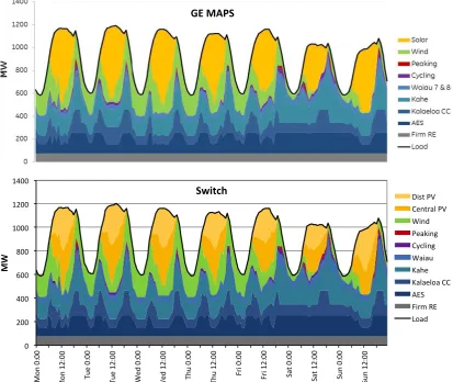
Hourly System Operation
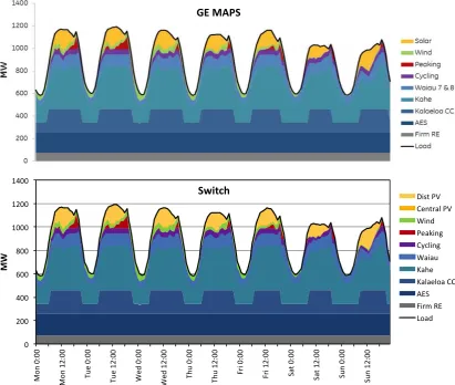
11 am to 3:59 pm on the Saturday and 8 am to 3:59 pm on the Sunday, while MAPS commits two cycling plants during these times. In both cases the cycling plant(s) run at minimum load (22.5 MW each), and pri-marily provide reserves. Switch also decommits some Kalaeloa capacity earlier than MAPS on the last even-ing.
We could not identify a reason for the discrepancies in the hourly profiles from the two models. It is possible they are caused by different treatments of minimum up-/down-times for power plants (on the Satur-day, one cycling unit exactly meets both of these limits), or MAPS may have been configured to optimize commitment beyond the minimum needed for load and reserves (Switch was configured to commit only the minimum required capacity).
We also note that MAPS slightly reduces output from Kalaeloa during the times of lowest power demand on Wednesday and Thursday nights, and this effect is slightly weaker in the Switch modeling. This suggests Switch may have used a lower minimum-load or down-reserve requirement for the Kahe and Waiau baseload units than MAPS.
Figure 5 compares hourly results for a high-renewable scenario (#16). Again the match is close overall, but Switch used slightly more baseload generation and less cycling generation than MAPS. For example, Switch decommits Kalaeloa 2 & 3 at midday on Tuesday, late morning on Wednesday and late evening on Sunday, while MAPS keeps them running. Switch also runs less cycling capacity (purple) than MAPS on Monday afternoon, Friday afternoon and at 6 pm on Saturday.
Figure 4. Hourly power production in Scenario 2 during the week of June 22–28, calculated by MAPS and Switch (plot begins on a Monday)
0 200 400 600 800 1000 1200 1400 Mon 0:0 0 Mon 12 :0 0 Tu e 0:0 0 Tu e 12:0 0 We d 0:0 0 We d 12:00 Thu 0:0 0 Thu 12:0 0 Fri 0: 0 0 Fri 12 :0 0 Sat 0:0 0 Sat 12 :0 0 Sun 0:0 0 Sun 12:00 MW
Switch DistPV
Figure 5. Hourly power production in Scenario 16 during the week of June 22–28, calculated by MAPS and Switch with standard model settings (plot begins on a Monday)
Generalizability
Other regions and models. As noted in the Background section, this study focused on replicating the
detailed findings from MAPS, as reported in the RPS Study. MAPS itself was calibrated based on actual operational practices on Oahu and Maui [57, 58]. Due to the unavailability of public data for MAPS in other regions or for other proprietary models in any region, we have not been able to perform a broader comparison of Switch against other models or in other regions. However, if Switch and other models are both calibrated to reflect local operational practices (as done here), we would expect similar results between them. Conse-quently, we recommend that users “ground-truth” power system models (whether open-source or proprietary) against local practices before conducting studies in any region. We also encourage modelers to publish their data and operating rules to support more intercomparisons in the future.
Larger networks. The RPS Study modeled only two zones (Oahu and Maui). As discussed in the
Trans-mission Network section, due to a lack of public network data, we ran Switch in flowgate mode for this study, with no losses or limits on flow within each zone, and finite, dispatchable transfer capability between zones. Flowgates are a fairly accurate representation of this particular power system—two regions with adequate internal transmission capacity joined by a controllable HVDC line—and the two models agreed fairly well about system operation. However, additional, future work is needed to judge whether the models perform similarly for power systems with many network buses, transmission congestion and security constraints. We have not yet identified a multi-node commercial study with enough public data to perform this assessment.
0 200 400 600 800 1000 1200 1400 Mon 0: 0 0 Mon 12 :00 Tue 0: 0 0 Tu e 12 :00 Wed 0: 0 0 We d 12 :0 0 Th u 0: 0 0 Th u 12 :0 0 Fr i 0:0 0 Fr i 12 :0 0 Sa t 0:00 Sa t 12 :0 0 Sun 0: 0 0 Sun 12: 00 MW
Switch DistPV
Conclusion
The commercial GE MAPS production cost model is widely used for renewable energy integration stud-ies, including the recent Hawaii Renewable Portfolio Standards Study (RPS Study) [59]. The goal of this model intercomparison was to test whether similar results could be obtained from the open-source Switch model when operated in production-cost mode and configured to study the same high-renewable power sys-tems.
We found that when Switch was configured similarly to MAPS, it produced results that were very close to MAPS, at least for the 17 scenarios evaluated here. Although the models agree closely, the agreement is not exact. The largest differences between the models are in the selection among different thermal power plants to provide power each hour. As noted in the Methods and Supplementary Information, there are a number of areas where Switch’s configuration may have differed from MAPS, possibly contributing to these differences. These areas include generator outages, calculation of down-reserve targets, allocation of reserve targets between islands, commitment order for Oahu and Maui power plants, commitment rules, treatment of the inter-island cable during unit commitment and dispatch, operating rules for Maui’s Maalaea combined-cycle plants, and variable cost of the Kalaeloa plant.
We are not able to judge which of these are the largest contributors, because the complete MAPS inputs and model are not available to the public. However, based on the qualitative similarity in findings between the models, we conclude that it is possible to configure Switch to obtain substantially similar results to MAPS, at least for the types of analysis reviewed here.
This study focused on replicating the detailed findings from MAPS, as reported in the RPS Study. Due to the unavailability of public data for MAPS in other regions or for other proprietary models in any region, we were not able to perform a broader comparison of Switch against other models or in other regions, but hope to do this in future work.
For this study, we ran Switch in flowgate mode, with no losses or limits on flow within each zone, and finite, dispatchable transfer capability between zones. Flowgates are a fairly accurate representation of this particular power system and the two models agreed fairly well about system operation here. However, addi-tional, future work is needed to judge whether the models perform similarly for power systems with many network buses, transmission congestion and security constraints.
As a general guideline, we recommend that researchers take care to ensure that their model assumptions match local practices and “ground-truth” their power system models (whether open-source or proprietary) against previous work or operational experience when conducting studies in a new region. We also encourage modelers to publish their data and operating rules to support more intercomparisons in the future.
Declarations
Ethics approval and consent to participate Not applicable.
Consent for publication Not applicable.
Availability of data and materials
All datasets, code and configuration files used for the current study, as well as installation instructions, are available in a public Github repository at https://github.com/switch-hawaii/ge_validation.
Competing interests
The author declares no competing interests.
Funding
Author’s contributions
M.F. conceived the study, conducted the study, analyzed the results and wrote the manuscript. The author read and approved the final manuscript.
Acknowledgements
The author is grateful to staff at the Hawaii Natural Energy Institute and the Florida Solar Center, espe-cially Katherine McKenzie, Kevin Davies and John Cole, for assistance in obtaining data and for providing valuable suggestions to help clarify the manuscript. Thanks also to Derek Stenclik at GE Energy Consulting for clarifying the approaches taken in the RPS Study. Any errors remain the author’s own.
Author’s information
M.F. is an Assistant Professor of Electrical Engineering at the University of Hawaii at Manoa, special-izing in optimal design of power systems with large shares of renewable energy, storage and demand re-sponse. He is the lead author of the open-source Switch power system software.
References
1. IPCC (2018) Global Warming of 1.5 °C: an IPCC special report on the impacts of global warming of 1.5 °C above pre-industrial levels and related global greenhouse gas emission pathways, in the context of strengthening the global response to the threat of climate change, sustainable development, and ef-forts to eradicate poverty. Intergovernmental Panel on Climate Change, Geneva, Switzerland, http://www.ipcc.ch/report/sr15/
2. Williams JH, DeBenedictis A, Ghanadan R, et al (2012) The Technology Path to Deep Greenhouse Gas Emissions Cuts by 2050: The Pivotal Role of Electricity. Science 335:53–59.
https://doi.org/10.1126/science.1208365
3. Fripp M, Johnston J, Henríquez R, Maluenda B (2018) Switch 2.0: a modern platform for planning high-renewable power systems. Preprint, https://arxiv.org/abs/1804.05481
4. Pfenninger S, Hawkes A, Keirstead J (2014) Energy systems modeling for twenty-first century energy challenges. Renewable & Sustainable Energy Reviews 33:74–86
5. Després J, Hadjsaid N, Criqui P, Noirot I (2015) Modelling the impacts of variable renewable sources on the power sector: Reconsidering the typology of energy modelling tools. Energy 80:486–495. https://doi.org/10.1016/j.energy.2014.12.005
6. Heaps C (2016) Long-range Energy Alternatives Planning (LEAP) system. Stockholm Environment Institute, Somerville, Massachusetts, https://www.sei.org/projects-and-tools/tools/leap-long-range-en-ergy-alternatives-planning-system/
7. Howells M, Rogner H, Strachan N, et al (2011) OSeMOSYS: the open source energy modeling sys-tem: an introduction to its ethos, structure and development. Energy Policy 39:5850–5870
8. Karlsson K, Meibom P (2008) Optimal investment paths for future renewable based energy systems— Using the optimisation model Balmorel. International Journal of Hydrogen Energy 33:1777–1787 9. Shawhan DL, Taber JT, Shi D, et al (2014) Does a detailed model of the electricity grid matter?
Esti-mating the impacts of the Regional Greenhouse Gas Initiative. Resource and Energy Economics 36:191–207
10. Hilpert S, Kaldemeyer C, Krien U, et al (2018) The Open Energy Modelling Framework (oemof) - A novel approach in energy system modelling. preprints.org manuscript/201706.0093/v2.
https://doi.org/10.20944/preprints201706.0093.v2
11. Dorfner J (2018) urbs: a linear optimisation model for distributed energy systems — urbs 0.7.1 docu-mentation. Chair of Renewable and Sustainable Energy Systems, Technical University of Munich, https://urbs.readthedocs.io/
12. Brown T, Hörsch J, Schlachtberger D (2018) PyPSA: Python for Power System Analysis. Journal of Open Research Software 6:. https://doi.org/10.5334/jors.188
14. E3 (2017) RESOLVE: Renewable Energy Solutions Model. Energy and Environmental Economics, Inc, San Francisco, California, http://www.ethree.com/tools/resolve-renewable-energy-solutions-model/
15. Behboodi S, Chassin DP, Crawford C, Djilali N (2016) Renewable resources portfolio optimization in the presence of demand response. Applied Energy 162:139–148. https://doi.org/10.1016/j.apen-ergy.2015.10.074
16. Palmintier BS, Webster MD (2016) Impact of Operational Flexibility on Electricity Generation Plan-ning With Renewable and Carbon Targets. IEEE Transactions on Sustainable Energy 7:672–684. https://doi.org/10.1109/TSTE.2015.2498640
17. van Stiphout A, de Vos K, Deconinck G (2017) The impact of operating reserves on investment plan-ning of renewable power systems. IEEE Transactions on Power Systems 32:378–388.
https://doi.org/10.1109/TPWRS.2016.2565058
18. O’Neill RP, Krall EA, Hedman KW, Oren SS (2013) A model and approach to the challenge posed by optimal power systems planning. Math Program 140:239–266. https://doi.org/10.1007/s10107-013-0695-3
19. GE Energy (2010) Western Wind and Solar Integration Study. Prepared for the National Renewable Energy Laboratory, Golden, Colorado, http://www.nrel.gov/docs/fy10osti/47434.pdf
20. Bloom A, Townsend A, Palchak D, et al (2016) Eastern Renewable Generation Integration Study. http://dx.doi.org/10.2172/1318192
21. Foley AM, Ó Gallachóir BP, Hur J, et al (2010) A strategic review of electricity systems models. En-ergy 35:4522–4530. https://doi.org/10.1016/j.enEn-ergy.2010.03.057
22. GE Energy Consulting (2014) Minnesota Renewable Energy Integration and Transmission Study: Fi-nal Report. GE Energy Consulting in collaboration with MISO,
http://mn.gov/commerce-stat/pdfs/mrits-report-2014.pdf
23. Ma O, Cheung K (2016) Demand Response and Energy Storage Integration Study. U.S. Department of Energy, Washington, D.C., https://www.energy.gov/sites/prod/files/2016/03/f30/DOE-EE-1282.pdf 24. GE Energy (2011) Oahu Wind Integration Study: Final Report. Hawaii Natural Energy Institute and
School of Ocean and Earth Science and Technology, University of Hawaii, Honolulu, Hawaii, https://www.hnei.hawaii.edu/sites/www.hnei.hawaii.edu/files/Oahu%20Wind%20Integra-tion%20Study.pdf
25. GE Energy (2012) Hawaii Solar Integration Study: Final Technical Report for Oahu. Prepared for the National Renewable Energy Laboratory, Hawaii Natural Energy Institute, Hawaii Electric Company and Maui Electric Company, Honolulu, Hawaii, http://www.hnei.hawaii.edu/sites/dev.hnei.ha-waii.edu/files/120401%20HSIS%20Oahu%20Technical%20Report_Final.pdf
26. Johal H, Hinkle G, Stenclik D, et al (2014) Hawaii RPS Roadmap Study Presentation. GE Energy Con-sulting and Hawaii Natural Energy Institute, Honolulu, Hawaii,
http://www.hnei.ha-waii.edu/sites/dev.hnei.hawaii.edu/files/news/Full%20Slide%20Deck.pdf
27. Jaske M, Wong L (2013) Summary of Studies of Southern California Infrastructure. California Energy Commission, Sacramento, California, http://www.energy.ca.gov/2013_energypolicy/documents/2013-07-15_workshop/background/Summary_of_Studies_of_Sourthern_California_Infrastructure.pdf 28. Wilson G, Aruliah DA, Brown CT, et al (2014) Best Practices for Scientific Computing. PLOS
Biol-ogy 12:
29. DeCarolis JF, Hunter K, Sreepathi S (2012) The case for repeatable analysis with energy economy op-timization models. Energy Economics 34:1845–1853
30. Leopoldina, acatech, Akademienunion (2016) Consulting with energy scenarios: requirements for sci-entific policy advice. German National Academy of Sciences Leopoldina, acatech – National Academy of Science and Engineering and Union of the German Academies of Sciences and Humanities, Ger-many, https://www.acatech.de/Publikation/consulting-with-energy-scenarios-requirements-for-scien-tific-policy-advice/
32. Camerer C, Dreber A, Holzmeister F, et al (in press) Evaluating the Replicability of Social Science Ex-periments in Nature and Science between 2010 and 2015. Nature Human Behavior
33. Jacob D, Bärring L, Christensen OB, et al (2007) An inter-comparison of regional climate models for Europe: model performance in present-day climate. Climatic Change 81:31–52.
https://doi.org/10.1007/s10584-006-9213-4
34. Smith WN, Grant BB, Campbell CA, et al (2012) Crop residue removal effects on soil carbon: Meas-ured and inter-model comparisons. Agriculture, Ecosystems & Environment 161:27–38.
https://doi.org/10.1016/j.agee.2012.07.024
35. Mirsadeghi M, Blocken B, Hensen JLM (2008) Validation of external BES-CFD coupling by inter-model comparison. In: Proceedings of 29th AIVC Conference, Kyoto, Japan. Kyoto, Japan, p https://pure.tue.nl/ws/files/2966441/713596863518486.pdf
36. Lobell DB, Bonfils C, Duffy PB (2007) Climate change uncertainty for daily minimum and maximum temperatures: A model inter-comparison. Geophysical Research Letters 34:.
https://doi.org/10.1029/2006GL028726
37. Friedlingstein P, Cox P, Betts R, et al (2006) Climate–Carbon Cycle Feedback Analysis: Results from the C4MIP Model Intercomparison. J Climate 19:3337–3353. https://doi.org/10.1175/JCLI3800.1 38. Rosenzweig C, Elliott J, Deryng D, et al (2014) Assessing agricultural risks of climate change in the
21st century in a global gridded crop model intercomparison. PNAS 111:3268–3273. https://doi.org/10.1073/pnas.1222463110
39. Gregory JM, Bouttes N, Griffies SM, et al (2016) The Flux-Anomaly-Forced Model Intercomparison Project (FAFMIP) contribution to CMIP6: investigation of sea-level and ocean climate change in re-sponse to CO₂ forcing. Geoscientific Model Development 9:3993–4017
40. Fripp M (2008) Optimal investment in wind and solar power in California. Energy and Resources Group, University of California, Berkeley, Berkeley, http://gradworks.umi.com/33/88/3388273.html 41. Nelson J, Johnston J, Mileva A, et al (2012) High-resolution modeling of the western North American
power system demonstrates low-cost and low-carbon futures. Energy Policy 43:436–447
42. Barido DP de L, Johnston J, Moncada MV, et al (2015) Evidence and future scenarios of a low-carbon energy transition in Central America: a case study in Nicaragua. Environ Res Lett 10:104002.
https://doi.org/10.1088/1748-9326/10/10/104002
43. He G, Avrin A-P, Nelson JH, et al (2016) SWITCH-China: A Systems Approach to Decarbonizing China’s Power System. Environ Sci Technol 50:5467–5473. https://doi.org/10.1021/acs.est.6b01345 44. Kammen DM, Shirley R, Carvallo JP, Barido DP de L (2014) Switching to Sustainability. Berkeley
Review of Latin American Studies
45. Wakeyama T (2015) Impact of Increasing Share of Renewables on the Japanese Electricity System - Model Based Analysis. Energynautics GmbH, Brussels, Belgium
46. Fripp M (2016) Making an Optimal Plan for 100% Renewable Power in Hawaii - Preliminary Results from the SWITCH Power System Planning Model. University of Hawaii Economic Research Organi-zation (UHERO), Honolulu, Hawaii, http://www.uhero.hawaii.edu/assets/WP_2016-1.pdf
47. Imelda, Fripp M, Roberts MJ (2018) Variable pricing and the cost of renewable energy. National Bu-reau of Economic Research, Cambridge, Massachusetts, http://www.nber.org/papers/w24712 48. Switch Authors (2018) Switch Power System Planning Model. GitHub repository
https://github.com/switch-model
49. Porter K, IAP Team (2007) Intermittency Analysis Project: Final report. California Energy Commis-sion, Sacramento, CA, http://www.energy.ca.gov/pier/final_project_reports/CEC-500-2007-081.html 50. Corbus D, Schuerger M, Roose L, et al (2010) Oahu Wind Integration and Transmission Study:
Sum-mary Report. National Renewable Energy Laboratory, Golden, Colorado, http://www.nrel.gov/docs/fy11osti/48632.pdf
52. Piwko R, Roose L, Orwig K, et al (2012) Hawaii Solar Integration Study: Solar Modeling Develop-ments and Study Results. National Renewable Energy Laboratory, Golden, Colorado,
http://www.nrel.gov/docs/fy13osti/56311.pdf
53. GE Energy Consulting (2014) PJM Renewable Integration Study. Prepared for PJM Interconnection, LLC, https://www.pjm.com/~/media/committees-groups/subcommittees/irs/postings/pjm-pris-task-3a-part-a-modeling-and-scenarios.ashx
54. Bebic J, Hinkle G, Matic S, Schmitt W (2015) Grid of the Future: Quantification of Benefits from Flexible Energy Resources in Scenarios With Extra-High Penetration of Renewable Energy. GE En-ergy Consulting, https://www.osti.gov/scitech/biblio/1339431
55. GE Energy Consulting (2013) Nova Scotia Renewable Energy Integration Study. Prepared for Nova Scotia Power, Inc., https://www.nspower.ca/site/media/Parent/2013COSS_CA_DR-14_SUPPLE-MENTAL_REISFinalReport_REDACTED.pdf
56. Ellison J, Bhatnagar D, Karlson B (2012) Maui Energy Storage Study. Sandia National Laboratories, Albuquerque, New Mexico, and Livermore, California,
http://www.sandia.gov/ess/publica-tions/SAND2012-10314.pdf
57. GE Global Research, HNEI, SOEST (2009) O’ahu Grid Study: Validation of Grid Models. GE Global Research, Hawaii Natural Energy Institute and School of Ocean and Earth Science and Technology, University of Hawaii,
http://www.hnei.hawaii.edu/sites/www.hnei.ha-waii.edu/files/Oahu%20Grid%20Study.pdf
58. GE Global Research, HNEI, SOEST (2008) Maui Electrical System Simulation Model Validation. GE Global Research, Hawaii Natural Energy Institute and School of Ocean and Earth Science and Tech-nology, University of Hawaii,
http://www.hnei.hawaii.edu/sites/dev.hnei.ha-waii.edu/files/081117%20Task%209%20Deliverable.pdf
59. GE Energy Consulting (2015) Hawaii Renewable Portfolio Standards Study. Hawaii Natural Energy Institute and School of Ocean and Earth Science and Technology, University of Hawaii,
http://www.hnei.hawaii.edu/projects/hawaii-rps-study
60. Fripp M (2018) Software and data repository for Switch-GE MAPS model intercomparison. https://github.com/switch-hawaii/ge_validation. Accessed 3 Aug 2018
61. Stenclik D (2017) Personal communication 8/22/2017 62. Stenclik D (2016) Personal communication 9/28/2016
63. Coffman M, Bernstein P, Wee S (2014) Cost Implications of GHG Regulation in Hawai‘i. University of Hawaii Economic Research Organization (UHERO), Honolulu, Hawaii, http://www.uhero.ha-waii.edu/assets/WP_2014-5.pdf